Evidence for Genetic Control of Adult Weight Plasticity in the Snail Helix aspersa

Abstract

Phenotypic plasticity and canalization are important topics in quantitative genetics and evolution. Both concepts are related to environmental sensitivity. The latter can be modeled using a model with genetically structured environmental variance. This work reports the results of a genetic analysis of adult weight in the snail Helix aspersa. Several models of heterogeneous variance are fitted using a Bayesian, MCMC approach. Exploratory analyses using posterior predictive model checking and model comparisons based on the deviance information criterion favor a model postulating a genetically structured heterogeneous environmental variance. Our analysis provides a strong indication of a positive genetic correlation between additive genetic values affecting the mean and those affecting environmental variation of adult body weight. The possibility of manipulating environmental variance by selection is illustrated numerically using estimates of parameters derived from the snail data set.

PHENOTYPIC plasticity and its counterpart, phenotypic stability, are concepts related to environmental sensitivity and play important roles in mechanisms linked to adaptation and evolution (Falconer and Mackay 1996; Roff 1997). Important questions from a breeding point of view are related to performance of plants or domestic animals under either homogeneous environments (often associated with intensive production systems) or a wide range of environmental conditions. The latter are often low-input production systems. From an evolutionary point of view, one is interested in understanding the processes by which organisms adapt and genetic variation is maintained in complex, temporally or spatially changing environments.

Environmental sensitivity can be defined either as mean phenotypic changes of a given genotype in different environments or as differences in the residual variance of different genotypes in the same environment (Jinks and Pooni 1988). These two definitions give rise to two different genetic statistical models. In the first one, the phenotypic expression of a particular genotype is assumed to depend on the type of environment the individual is exposed to. One typically has specific types of environment in mind, for example, low and high temperature. Then the phenotypic plasticity of a genotype, defined by the relationship between phenotype and the environment, can be described by including a genetic component in a regression model, i.e., using a so-called reaction-norm model (see, e.g., Gavrilets and Scheiner 1993a,b). The second definition of environmental sensitivity gives rise to a model for residual variation. Given the genotype of an individual a certain value of the phenotype is expected. In practice the observed phenotype differs from the expected phenotype and this deviation may be attributed to the sum of influences of all the environmental conditions that the individual has been exposed to from the time of conception. The deviation is then modeled as random residual noise, whose variation may be a function of covariates and of a genetic component. In this model, different genotypes confer a difference in both mean and residual (or environmental) variation.

Several experiments have been conducted to elucidate whether environmental sensitivity is under genetic control. In the context of phenotypic plasticity/stability Waddington (1960), for example, demonstrated that it is possible to select for phenotypic stability toward different temperature environments. Specifically, Waddington (1960) selected for number of eye facets in bar-eyed Drosophila mutants in two rearing environments: 18° and 25°. Unselected individuals reared at 18° had 182% more facets than those reared at 25°. Selection for stability to variations of the environment was performed by splitting each family in two (one part reared at 18°, the other at 25°). The family average differences were used to select the less sensitive animals. After five generations of selection the difference in mean number of eye facets in the two environments was reduced to 11%. Another divergent selection experiment in Drosophila involving plasticity of thorax size in two different temperatures (19° and 25°) produced very significant responses in both the upward and the downward direction (Scheiner and Lyman 1991). Empirical results like these require modeling environmental sensitivity at the level of the mean.

We are here concerned with the second interpretation above of environmental sensitivity. In this case a number of models describing genetic control of environmental or residual variance have been studied. Early models assumed that residual variance decreases with the number of heterozygous loci (Lerner 1954; Lewontin 1964; Zhivotovsky and Feldman 1992). An extension postulates that a finite number of loci have pleiotropic effects on the mean and variance (Gavrilets and Hastings 1994; Hill 2002). Recently, San Cristobal-Gaudy et al. (1998) proposed an infinitesimal model with a genetically structured residual variance, thus generalizing the classical infinitesimal model used in quantitative genetics (Fisher 1918). With the exception of recent work by Garreau et al. (2003) and Sorensen and Waagepetersen (2003), there is limited convincing experimental evidence for genetic control of residual variability.

In this article we report results of an analysis of adult weight in a nonlaboratory species, the snail Helix aspersa. The objective is to investigate whether the residual variance of adult weight is under genetic control. The data are analyzed with the genetically structured residual variance model proposed by San Cristobal-Gaudy et al. (1998), based on earlier work of Foulley and Quaas (1995). Maximum-likelihood inference for this model is highly intractable. Instead we implement a Bayesian inference using Markov chain Monte Carlo (MCMC) as proposed by Sorensen and Waagepetersen (2003).

MATERIALS AND METHODS

The data:

H. aspersa snails are protandrous hermaphrodites: the males mate, fertilizing each other, and later both turn into females. Under our experimental conditions, ∼130 eggs on average are laid by each pair of snails (Bonnet et al. 1990). The definition of sexual maturity was the standard one based on judging whether the peristome (edge of the aperture of the shell) was reflected. A sexually mature snail weighs 10 g on average with an empirical standard deviation of 1.8 g and is 8–20 weeks old.

The data consist of 22,033 adult weights collected over 11 discrete generations, spanning the period from 1991 until 2002. Animals were reared at the experimental unit of INRA-Le Magneraud. The line was maintained with 120 animals chosen from 30 families, with an equal number from each family. Mating among the 120 snails was at random, with the restriction that full-sibs were not allowed to mate. Even though the 120 parents should have been randomly chosen with respect to weight by design, a slight positive trend was detected (not shown), presumably because larger snails are easier to pick than smaller ones. The pedigree file includes 22,454 individuals.

Animals were housed in a room kept at a temperature/relative humidity of 20°/70% during the day and 17°/90% during the night. Feeding was ad libitum with a commercial compound feed. Further details about rearing conditions are given in Dupont-Nivet et al. (1997). After eclosion, snails were maintained in boxes of 30 individuals during the growth period and boxes were randomly distributed over shelves. Animals were checked once a week for peristome reflection, and those that were judged to have reached the appropriate weight were placed in a starving box for 3 days before being weighed to the nearest 0.01 g.

Model with genetically structured variance heterogeneity:

The analysis is based on the model introduced by San Cristobal-Gaudy et al. (1998). It is assumed that conditionally on vectors of location and dispersion parameters, the vector of the n phenotypes (adult weights) is Gaussian,

1

where diag is a diagonal matrix with diagonal entries σ²_i,

and

The vectors b and b* contain effects associated with generation (11 levels) and whether each of the two snails laid eggs or not (2 levels) and X, Z, and W are known incidence matrices. The genetic effects (a′, a*′) are assumed to be Gaussian,

2

where A is the additive genetic relationship matrix, σ²_a is the additive genetic variance affecting mean adult weight, σ²_a* is the additive genetic variance affecting environmental variance of adult weight, and ρ is the coefficient of genetic correlation. The vectors p and p* contain box effects on body weight and log-variance, respectively, and are assumed to be independent with

where n_box is the number of boxes used in the experiment. This model is labeled model 4. We also fitted three other models of decreasing complexity: model 3 is as model 4 but without a*, model 2 is as model 3 but without p*, and model 1 is the standard linear mixed model with homogeneous residual variance [i.e., in model 1 the residual variances σ²_i are all equal to exp(b*) for some parameter b*].

The phenotypic variance is the variance of the conditional distribution of y_i given b and b*, and the heritability parameter h² is the usual ratio of additive to phenotypic variance. Under model 4, these parameters are

3

and

4

respectively, where (Xb*)_i is the ith row of Xb*. The parameter h² features in the response to selection for the mean of the trait (Sorensen and Waagepetersen 2003). The third central moment is

5

The conditional distribution of y_i given b and b* therefore has negative, zero, or positive skewness,

6

depending on whether ρ is negative, zero, or positive.

In our statistical analysis we use the Bayesian approach described in Sorensen and Waagepetersen (2003). A priori b and b* were assigned normal distributions with zero mean vector and diagonal matrix with very large diagonal elements. The variance parameters σ²_a, σ²_a*, σ²_p, and σ²_p* were assigned scaled inverted chi-square distributions and ρ was assigned a uniform prior bounded between −1 and 1. Posterior distributions are computed using the MCMC algorithm proposed by Sorensen and Waagepetersen (2003), where further details concerning the model and its implementation can be found. Briefly, the vector b was sampled using a Gibbs update, and the vectors (a′, a*′) and (p′, p*′) were reparameterized with the intention of reducing their posterior correlation and sampled subsequently using Metropolis-Hastings with Langevin-Hastings proposals. The vector b* was sampled using Metropolis-Hastings with a Langevin-Hastings proposal as well, and the log-variance components and the correlation coefficient were sampled using Metropolis-Hastings with random-walk proposals.

In the rest of the article, the residual variance, that is, the variance of the conditional distribution of the data, given the parameters and the model, is interpreted and referred to as the environmental variance.

RESULTS

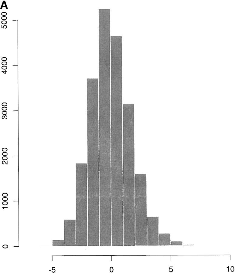
Figure 1A shows a histogram of the 22,033 residuals obtained from a least-squares analysis, accounting for generation effects and for egg-laying pattern. The histogram displays a heavy tail to the right, which is indicative of a positive genetic correlation ρ under the San Cristobal-Gaudy et al. (1998) model, cf. (5) and (6).

Figure 1.—

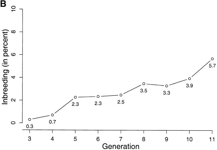
(A) Residuals from a least-squares analysis of adult weights. (B) Average percentage of inbreeding per generation, from generations 3–11.

To give an idea of the effective population size, average inbreeding coefficients per generation are shown in Figure 1B. The average effective size implied by Figure 1 is of ∼94 breeding individuals per generation.

Inferences about chosen parameters based on the four models fitted:

The results reported for each model are obtained from MCMC runs consisting of between 4,000,000 and 12,000,000 iterations. Table 1 shows Monte Carlo estimates of posterior means and Monte Carlo estimates of 95% posterior intervals for chosen parameters based on models 1, 2, 3, and 4. The Monte Carlo estimates of the posterior means of b* and of exp(b*) based on model 1 are 0.003 and 1.00, respectively (not shown in Table 1). For models 2–4, the parameters b^*_egg and b^*_1,11 are, respectively, the effects on the log-environmental variance of moving from level 1 to 2 for the egg factor and from level 1 to 11 for the generation factor. The estimates of the posterior means for the various components of variance are fairly stable across models, perhaps with the exception of σ²_a that shows an increase in going from model 1 to 2 and σ²_p* that decreases going from model 3 to 4 (the latter is to be expected since model 4 includes an additional variance component σ²_a*). To give an idea of the precision of the Monte Carlo computations we show in the final row confidence intervals for the estimated posterior means under model 4, reflecting Monte Carlo noise.

TABLE 1.

Monte Carlo estimates of posterior means (first row for each model) and of 95% posterior intervals (second row for each model) of chosen parameters of models 1, 2, 3, and 4

Model	b*egg	b*1,11	σ2a	σ2p	σ2a*	σ2p*	ρ
1	—	—	1.70	0.49	—	—	—
—	—	1.50; 1.90	0.43; 0.55	—	—	—
2	−0.16	−0.45	1.84	0.48	—	—	—
−0.25; −0.06	−0.65; −0.25	1.60; 2.07	0.42; 0.53	—	—	—
3	−0.13	−0.43	1.70	0.46	—	0.39	—
−0.25; −0.01	−0.69; −0.20	1.51; 1.86	0.41; 0.52	—	0.30; 0.49	—
4	−0.02	−0.82	1.71	0.47	0.29	0.17	0.81
−0.15; 0.10	−1.20; −0.45	1.62; 1.81	0.41; 0.52	0.23; 0.35	0.14; 0.21	0.73; 0.87
	−0.03; −0.02	−0.90; −0.75	1.70; 1.72	0.46; 0.47	0.29; 0.30	0.17; 0.18	0.79; 0.82

The third row of model 4 shows confidence intervals for the estimated posterior means, reflecting Monte Carlo sampling variance. b^*_egg (b^*_1,11), egg effect (generation effect); σ²_a (σ²_a*), additive variance at the level of the mean (variance); σ²_p (σ²_p*), variance due to box effects at the level of the mean (variance); ρ, genetic correlation.

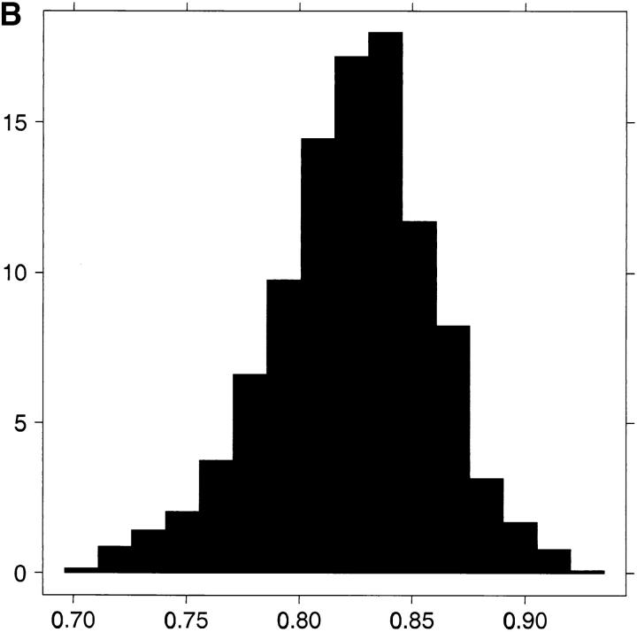
A few interesting observations can be derived from the numbers in Table 1. One is the rather high proportion of additive genetic variation at the level of the mean of the trait. Thus, under model 4 the posterior mean/credibility interval of h² = 0.63 (0.59; 0.68) for generation 11 and level 2 of egg. For generation 1 and level 2 of egg we obtain 0.51 (0.48; 0.55). Under model 1, the numbers are 0.53 (0.46; 0.58). The result under model 1 is in agreement with that in Dupont-Nivet et al. (1997). The other interesting observation pertains to ρ whose posterior mean of 0.81 and rather tight credibility interval disclose a large positive additive genetic association between genetic values affecting the mean of the trait and those affecting its environmental variation. The estimated posterior distribution of ρ is shown in Figure 2B.

Figure 2.—

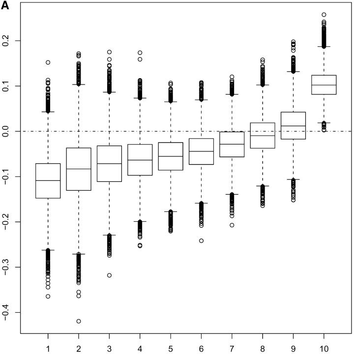
(A) Boxplots for posterior MCMC realizations (under model 3) of averaged squared standardized residuals plotted against index of 10 groups of additive genetic values ordered according to increasing size. (B) Estimated marginal posterior distribution for ρ under model 4.

Assessment of models and priors:

Graphical evidence in support of model 4 showing a positive association between environmental variation and additive genetic values affecting mean adult weight is provided in Figure 2A. The plot is obtained under model 3 as follows. Conditional on parameters and random effects we define averaged squared standardized residuals,

7

where m_Ij is the number of observations with a_i ∈ I_j and I_j = [t_j, t_j+1[ are subintervals of the real line with −∞ = t₁ < t₂ < · · · < t₁₀ < t₁₁ = ∞ and t_j = −1.6 + 0.4(j − 2), j = 2, … , 10. In each Monte Carlo round, the sampled additive genetic values are ordered from the smallest to the largest in these intervals. Thus T_j measures the average environmental variation in groups obtained by ordering the observations according to the size of the Monte Carlo sampled genetic values a_i. To assess whether the observed values of T_j are consistent with the assumptions of model 3 one might check whether the observed T_j are atypical compared with their sampling distributions, which are χ²m_Ij/m_Ij under model 3. Equivalently one might check whether zero is an atypical value for the differences

where T^rep_j is χ²m_Ij/m_Ij. In practice, of course, the random effects and parameters are unknown so we use the idea of posterior predictive model checking (Rubin 1984; Gelman et al. 1996) and consider the posterior predictive distribution of T_j − T_j^rep. The boxplots in Figure 2A obtained from MCMC samples of the posterior predictive distributions of T_j − T_j^rep exhibit an increasing trend that is indicative of a positive association between environmental variation and additive genetic values affecting mean adult weight, as postulated by the fitted model 4. More details on this approach to posterior predictive model checking are provided in Sorensen and Waagepetersen (2003).

The four models fitted are compared using the deviance information criterion (DIC), recently proposed by Spiegelhalter et al. (2002). Briefly, the DIC is a measure that combines the fit of a model with its complexity, where the latter involves the number of parameters. Smaller values indicate a “better” model. The Monte Carlo estimates of the differences DIC_i − DIC₁ are −1629, −5327, and −5692, respectively, where DIC_i is the DIC for model i, i = 2, 3, 4. Spiegelhalter et al. (2002) suggest that differences in DIC >7 should be taken as important. Thus, in agreement with the posterior predictive model, checking the comparison based on the DIC favors model 4.

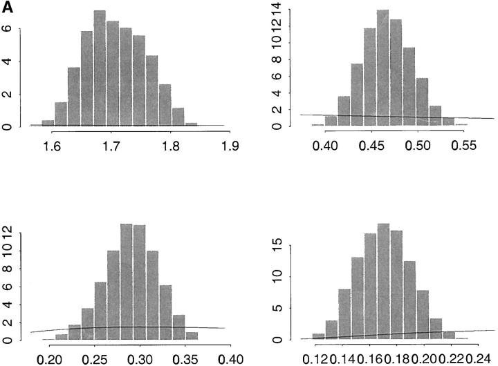
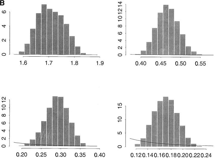
Figure 3 shows the estimated marginal posterior distributions of σ²_a, σ²_p, σ²_a*, and σ²_p* based on model 4. The solid lines superimposed on each plot of the figure represent the density of the prior νSχ⁻²_ν scaled inverted chi-square distribution of the parameters, where ν and S are degrees of freedom and the scale parameter, respectively, assumed known. For the four histograms of Figure 3A the parameters of the prior distributions are ν = 4 and S = 0.45. This results in a prior mode equal to 0.30. To study the influence of the prior distribution on the inferences, we considered also S = 0.05, which gives a prior mode equal to 0.033. The estimated marginal posterior distributions of the same parameters under this prior are shown in Figure 3B. The results under the two different prior assumptions are almost indistinguishable so our results appear to be rather insensitive to the choice of these priors.

Figure 3.—

(A, top) Monte Carlo estimates of σ²_a (additive genetic variance at the level of the mean) and σ²_p (variance due to box effects at the level of the mean); bottom, σ²_a* (additive genetic variance at the level of the variance) and σ²_p* (variance due to box effects at the level of the variance). The lines represent the prior νSχ⁻²_ν densities for the variances with parameters ν = 4 (degrees of freedom) and S = 0.45 (scale parameter). (B) Plots are as in A but with alternative choice of prior (ν = 4 and S = 0.05).

Assessment of mean-variance relation:

As mentioned in Sorensen and Waagepetersen (2003),

where u = a* − E[a*|a] is N0, σ²_a*1 − ρ²A and independent of a. Our model thus postulates a linear, stochastic relationship between the mean and the log-variance. It is precisely the presence of the stochastic term u that opens the possibility of changing the environmental variance by selection, without changing the mean. Note that |ρ| = 1 (corresponding to u = 0) results in a deterministic relationship between mean and variance.

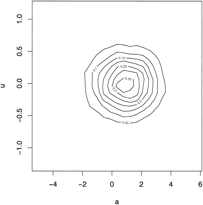
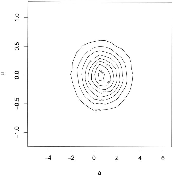
A further criticism of the postulated model could focus on the choice of functional relationship between mean and variance. If the choice of the log function is appropriate then the posterior results and the DIC give strong evidence for the presence of u/a*. However, a wrong choice of functional relationship might induce spurious results where variation in u could occur to compensate for the wrong functional relationship. This is not implied by Figure 2A, which, with the exception of the last interval, shows a fairly steady linear trend. The plots of posterior realizations of u vs. corresponding posterior realizations of a in Figure 4 give further support for a lack of systematic relation between the values of u and a.

Figure 4.—

Kernel-smoothed scatter plots of posterior realizations of u (vector of deviations of realized values of additive genetic effects affecting the variance, from their conditional expectations, given a; see Assessment of mean-variance relation) vs. corresponding posterior realizations of a (vector of additive genetic values affecting the mean). Both plots are based on independent posterior realizations of (a′, u′).

DISCUSSION

This work provides evidence that environmental variance for adult weight in the snail H. aspersa is partly under genetic control, as postulated by model 4. This conclusion is supported, first, by the posterior predictive model-checking study. We constructed discrepancy statistics specifically designed to test for genetically structured variance heterogeneity, and the test was positive (see Figure 2A). Further, the validity of the functional form of the mean-variance relationship postulated by model 4 was checked by plotting posterior realizations of u vs. those of a (see Figure 4). The lack of systematic relation between the values of u and a does not lead to questioning the adequacy of the exponential relationship.

Second, the model comparisons based on the DIC criterion (Spiegelhalter et al. 2002) favored model 4. Third, the posterior distribution of σ²_a* and of the genetic correlation are shifted a long way from zero (see Figure 3A and Figure 2B). In particular, Figure 2B must be seen in connection with Figure 3A. Indeed, the posterior analysis indicates that additive genetic values affecting environmental variance are strongly, positively correlated (posterior mean of ρ = 0.81, see also Table 1) with those affecting mean adult weight.

According to the inferred model 4, the genetic contribution to heterogeneity of environmental variance is of considerable magnitude: given σ²_a*, each component of a* is a priori N0, σ²_a*. Replacing σ²_a* by the posterior mean equal to 0.29 leads to an a priori 95% confidence interval for a component of a* ranging from −1.06 to 1.06. This corresponds to a ratio exp(1.06)/exp(−1.06) = 8 between the environmental variances for components of a* in the lower and upper ends of the confidence interval.

A referee raised the important point of whether the simple model 1 might be appropriate for log-transformed data since the log-transformation is often used to remove variance heterogeneity. Indeed, one might even consider the whole class of Box-Cox transformations (Box and Cox 1964), which is commonly used for analysis of positive-valued data. The study of the interplay between variance heterogeneity and possibly heavy-tailed sampling distributions is a research project in its own right. We here confine ourselves to considering the results of fitting model 4 to log- and square-root-transformed data for which residuals from least-squares analyses were heavy tailed to the left and close to symmetric, respectively. The posterior distributions provide evidence of genetic variance heterogeneity for both transformed data sets with a positive ρ for the square-root-transformed data and a negative ρ for the log-transformed data. This result can be explained by employing a Taylor series expansion to approximate the variance of the transformed data. Choosing between the different transformations may be viewed as a model selection exercise. According to the DIC, the best fit is obtained using the untransformed data.

The possibility of manipulating environmental variation via selection, conditionally on the inferred parameters of model 4 and the data, can be studied as follows. Consider directional selection of, for example, 240 snails out of the initial 2195 snails available in the data. The maximum possible (negative) response in the environmental variance is obtained when selection is based on the smallest ranking posterior means of the additive genetic values affecting environmental variation (i.e., the smallest E[a*|y]), disregarding the posterior means of the additive genetic values controlling mean adult weight (i.e., E[a|y]). The change in E[a*|y] translates into a reduction of the environmental variance of 43%, with a correlated reduction in the mean adult weight of ∼13%. We may alternatively consider a restricted index I = a* + ka with k chosen so that Cov(a, I) = 0. Then, upon replacing the unknown quantities with their posterior means, selection based on I should leave mean adult weight approximately unchanged (a more refined criterion of selection would involve using the posterior mean of the index, computed via MCMC). Selection of the 240 snails on this index generates a change in E[a*|y] that translates into a reduction in environmental variance of 22%. If the same exercise is carried out among the 2376 snails composing the next generation, the corresponding figures are very similar: 44 and 13% for the reduction of environmental variance and mean adult weight vs. a reduction in the former of 22% using the restricted index. Thus, given model 4, it seems possible to act on the environmental variance without changing mean adult weight, despite the high correlation between additive genetic values affecting mean and environmental variation (the empirical correlation between Monte Carlo estimates of E[a|y] and E[a*|y] among the 2195 snails and among the 2376 snails is 0.91). These numbers are indeed encouraging with respect to the prospects for controlling environmental variation by means of selection. However, they do not carry the same strength of evidence as that provided by a well-designed selection experiment. To the best of our knowledge, such an experiment has not been reported; it would be a welcome contribution to the literature on this important topic.

References

- Bonnet, J. C., P. Aupinel and J. L. Vrillon, 1990 L'escargot Helix aspersa: Biologie - élevage. Du labo au terrain, Institut National de la Recherche Agronomique, France.
- Box, G. E. P., and D. R. Cox, 1964. An analysis of transformations. J. R. Stat. Soc. Ser. B 26: 211–252. [Google Scholar]
- Dupont-Nivet, M., J. Mallard, J. C. Bonnet and J. M. Blanc, 1997. Quantitative genetics of growth traits in the edible snail, helix aspersa muller. Genet. Sel. Evol. 29: 571–587. [Google Scholar]
- Falconer, D. S., and T. F. C. Mackay, 1996 Introduction to Quantitative Genetics. Longman, New York.
- Fisher, R. A., 1918. The correlation between relatives on the supposition of Mendelian inheritance. Trans. R. Soc. Edinb. 52: 399–433. [Google Scholar]
- Foulley, J. L., and R. L. Quaas, 1995. Heterogeneous variances in Gaussian linear models. Genet. Sel. Evol. 27: 211–228. [Google Scholar]
- Garreau, H., M. Sancritobal, J. Hurteau, L. Bodin, G. Saleil et al., 2003 Peut-on sélectionner sur l'homogénéité des poids à la naissance au sein d'une portée?: résultats préliminaires. 10èmes Journées de la Recherche Cunicole, Paris.
- Gavrilets, S., and A. Hastings, 1994. A quantitative genetic model for selection on developmental noise. Evolution 48: 1478–1486. [DOI] [PubMed] [Google Scholar]
- Gavrilets, S., and S. M. Scheiner, 1993. a The genetics of phenotypic plasticity. V. Evolution of reaction norm shape. J. Evol. Biol. 6: 31–48. [Google Scholar]
- Gavrilets, S., and S. M. Scheiner, 1993. b The genetics of phenotypic plasticity. VI. Theoretical predictions for directional selection. J. Evol. Biol. 6: 49–68. [Google Scholar]
- Gelman, A., X. L. Meng and H. Stern, 1996. Posterior predictive assessment of model fitness via realized discrepancies (with discussion). Stat. Sin. 6: 733–807. [Google Scholar]
- Hill, W. G., 2002 Direct effects of selection on phenotypic variability of quantitative traits. Seventh World Congress on Genetics Applied to Livestock Production, August 19–23, Montpellier, France, communication no. 19–02.
- Jinks, J. L., and H. S. Pooni, 1988 The genetic basis of environmental sensitivity. Proceedings of the 2nd International Conference on Quantitative Genetics, North Carolina State University, Raleigh, NC, pp. 505–522.
- Lerner, I. M., 1954 Genetic Homeostasis. Oliver & Boyd, Edinburgh.
- Lewontin, R. C., 1964. The interaction of selection and linkage. II. Optimal model. Genetics 50: 757–782. [DOI] [PMC free article] [PubMed] [Google Scholar]
- Roff, D. E., 1997 Evolutionary Quantitative Genetics. Chapman & Hall, London/New York.
- Rubin, D. B., 1984. Bayesianly justifiable and relevant frequency calculations for the applied statistician. Ann. Stat. 12: 1151–1172. [Google Scholar]
- San Cristobal-Gaudy, M., J. M. Elsen, L. Bodin and C. Chevalet, 1998. Prediction of the response to a selection for canalisation of a continuous trait in animal breeding. Genet. Sel. Evol. 30: 423–451. [Google Scholar]
- Scheiner, S. M., and R. F. Lyman, 1991. The genetics of phenotypic plasticity. II. Response to selection. J. Evol. Biol. 4: 23–50. [Google Scholar]
- Sorensen, D., and R. Waagepetersen, 2003. Normal linear models with genetically structured residual variance heterogeneity: a case study. Genet. Res. 82: 207–222. [DOI] [PubMed] [Google Scholar]
- Spiegelhalter, D. J., N. G. Best, B. P. Carlin and A. Van Der Linde, 2002. Bayesian measures of model complexity and fit (with discussion). J. R. Stat. Soc. Ser. B 64: 583–639. [Google Scholar]
- Waddington, C. H., 1960. Experiments on canalizing selection. Genet. Res. 1: 140–150. [Google Scholar]
- Zhivotovsky, L. A., and M. W. Feldman, 1992. On the difference between mean and optimum of quantitative characters under selection. Evolution 46: 1574–1578. [DOI] [PubMed] [Google Scholar]