Effect of Two- and Three-Locus Linkage Disequilibrium on the Power to Detect Marker/Phenotype Associations

Abstract

There has been much recent interest in describing the patterns of linkage disequilibrium (LD) along a chromosome. Most empirical studies that have examined this issue have concentrated on LD between collections of pairs of markers and have not considered the joint effect of a group of markers beyond these pairwise connections. Here, we examine many different patterns of LD defined by both pairwise and joint multilocus LD terms. The LD patterns we considered were chosen in part by examining those seen in real data. We examine how changes in these patterns affect the power to detect association when performing single-marker and haplotype-based case-control tests, including a novel haplotype test based on contrasting LD between affected and unaffected individuals. Through our studies we find that differences in power between single-marker tests and haplotype-based tests in general do not appear to be large. Where moderate to high levels of multilocus LD exist, haplotype tests tend to be more powerful. Single-marker tests tend to prevail when pairwise LD is high. For moderate pairwise values and weak multilocus LD, either testing strategy may come out ahead, although it is also quite likely that neither has much power.

THE hope behind association mapping is to use linkage disequilibrium (LD) as an indication of proximity of a marker to genes affecting the trait of interest. Markers that are in strong LD with a gene of interest should be close to that gene, so once these markers have been identified, an approximate location for the gene can be established. While this concept appears reasonable in theory, there are many issues that arise in practical applications. One trouble is that the stochastic nature of evolution causes a large variation in LD around its expected value. Because of this, two pairs of loci for which the expected levels of LD are the same on the basis of an initial state can exhibit very different amounts of LD over time. To understand better the relationship between LD and distance, empirical patterns of pairwise LD have been studied with great interest for different genomic regions and within different populations (see Ardlie et al. 2002 for a review). These studies have given us insight into this relationship, including how far useful levels of LD extend and how levels of LD change across the genome and from population to population. There has also been much recent interest in the topic of “LD blocks” within the genome (see Wall and Pritchard 2003 for a review).

While these empirical studies have provided us with useful information regarding the distribution of LD and the relationship between LD and distance in real populations, an additional problem arises in the general theory relating LD to distance that is not addressed by these types of studies. This issue is that, while we would like to use LD as an indicator of proximity, and thus are interested in reliable estimates of LD, the alleles at both loci must be available for examination to estimate LD directly. When one of the loci of interest is the gene that is being mapped, most likely the alleles of that gene are not known. Instead, association-mapping methods attempt to measure LD indirectly, using phenotype as a surrogate for the genotype at the gene. What is measured is the level of association between the phenotype and the marker alleles. This use of phenotype as a substitute for genotype at the gene has consequences for estimating LD. In doing this, the manner in which the gene acts (which directs the degree to which phenotype represents genotype) becomes confounded with the degree of LD between the loci. This confounding of LD with genetic effects plays a role in how successful association-mapping techniques can be. This is intuitively apparent when considering that it is likely that genes with small effects will be much more difficult to detect than genes with large effects. Thomson and Bodmer (1979) examined the relationship between HLA haplotypes and association with disease. They assumed a dominant genetic model with incomplete penetrance, but note that the theory applies to other specified models as well. Nielsen and Weir (1999) provide a theoretical framework under a general genetic model to describe the role genetic effects play in association-mapping techniques and how these forces combine with LD to influence the power of these tests. This work has been extended to haplotype-based methods (Nielsen and Weir 2001). Through this work it has become apparent that even if simple relationships between LD and distance do exist, these relationships can be distorted when examining marker/phenotype associations.

A number of investigators have examined the question of whether haplotype-based association tests may be more powerful than single-locus tests when performing mapping studies, with varying conclusions. On the basis of analytical results and power computations, Akey et al. (2000) suggest that haplotypes can significantly improve the power of association-mapping techniques. In contrast, simulation studies by Long and Langley (1999) and Kaplan and Morris (2001) found that single-marker tests provide at least as much power as haplotype-based approaches. Fallin et al. (2001) used statistically reconstructed haplotype frequencies for relating Alzheimer's disease with multiple SNPs on chromosome 19. They found examples of haplotype/disease associations that were not identified using single markers. Their results provide an example where haplotypes are more informative than a single-point analysis, even if the phase information is recovered by statistical techniques.

Conceivably, there are several biological reasons a haplotype-based approach may be beneficial. One possibility would be if the functional basis of disease susceptibility is due to the combined changes at several sites within a gene region. A well-known example of this is the APOE gene and its effect on late-onset Alzheimer's disease (AD; Brouwer et al. 1996). Three alleles at this gene exist in reasonably high frequencies in most populations and have a varying effect on susceptibility. These alleles are distinguished from one another by base changes at two SNPs, so that it is the two-SNP haplotype combination that defines the APOE alleles.

Another circumstance where haplotype-based tests may provide greater power than single-marker tests depends on the haplotype structure across the markers of interest, considered jointly. In single-marker association tests, pairwise LD between the alleles at the marker and the functional alleles is important. If two single-marker tests are performed individually, the two sets of pairwise LD between the markers and the gene both contribute individually. If, however, two-marker haplotypes are considered, three loci (the markers and the putative functional site) must be considered jointly. In addition to the two sets of pairwise LD between each marker and the functional site, there is an additional disequilibrium value that captures the haplotype patterns of all three loci together, after having adjusted for each pairwise term. This joint LD term provides additional information beyond the two-locus measures. For alleles k at locus 1, r at locus 2, and i at locus 3, the three-locus LD term can be expressed as

1

(Bennett 1954), where P_kri, p_k, π_r, and q_i are the haplotype and allele frequencies. Here D_kr, D_ki, and D_ri are the set of two-locus LD terms, with the usual expression for pairwise LD, D_ki = P_ki − p_kq_i. Various properties of this measure have been examined (Hill 1976; Thomson and Baur 1984).

Thomson and Bodmer (1979) discuss how this measure plays a role in haplotype-based association tests. They give some examples for which haplotype tests may provide information not available from single-marker tests and also provide examples in which they do not. An illustrative example of how this three-locus LD can affect an association test is the following. Assume that two diallelic markers (A and B) are to be tested in the region of a diallelic functional site. Four three-locus haplotypes exist in equal frequencies in the population: A-D-B (25%), A-X-b (25%), a-D-b (25%), and a-X-B (25%). In this situation, the D allele at the functional site has a population allele frequency of 50%. Examining the alleles at the A locus alone provides no new information regarding the alleles at the functional site; the frequency of a D allele conditional upon a specific allele at the A locus is still 50%. The same is true examining the B locus alone. The allele at the functional site can be predicted with complete certainty, however, if the haplotype of the two markers is known. This is an example where there is no LD between any pair of loci, but the three-locus LD is large. Because of this, single-marker tests of association would have no power to detect this gene, while a haplotype-based test would be quite powerful. The example given here is unlikely to occur in real data; however, it is possible to describe more realistic haplotype patterns with similar properties.

Most previous empirical studies of LD patterns have concentrated on combinations of pairwise measures and have not examined joint multilocus LD. This includes the majority of studies of LD blocks, which tend to examine pairwise LD either directly or via haplotype estimation procedures, which themselves rely on pairwise LD. It is the multilocus LD coefficients, however, that potentially allow a haplotype-based test to be “greater than the sum of its parts.” In this article, we are interested in addressing several issues related to multilocus LD patterns and association mapping. We compare the behavior of haplotype and single-marker tests under different patterns of pairwise and multilocus LD, both to determine if one type of test is, in general, more powerful and to determine how different patterns of LD influence these tests. In addition to the usual single-marker and haplotype-based case-control tests, we describe a novel haplotype-based test for association based on contrasting the level of LD among affected individuals to that among unaffected individuals. Our experiments are based on simulations, but we incorporate empirical observations regarding LD patterns using estimates from real data (Zaykin et al. 2002). These data are used both to determine a reasonable range of LD patterns and to depict the behavior of LD and the power to detect association with the various tests across a chromosomal region.

METHODS

In association mapping, we hope to capture information about proximity of a marker to an unknown gene by measuring the degree of association between the marker and the phenotype. For example, in the case-control test, marker allele, genotype, or haplotype frequencies among affected individuals (cases) are compared to those among unaffected individuals (controls). If these are significantly different, we hope this is an indicator of a nearby gene. In the transmission/disequilibrium test (TDT; Spielman et al. 1993), we examine transmission rates of marker alleles from heterozygous parents to affected offspring. If the transmission rates of these marker alleles deviate from the expected 50%, this is considered evidence that there is a gene nearby that influences susceptibility. The consequence of measuring marker/phenotype correlations to determine marker-gene correlations is that the manner in which a gene acts to affect phenotype becomes important. The role of genetic effects in association mapping has been formalized (Nielsen and Weir 1999, 2001). We briefly summarize these results here.

We consider a gene, A, with an arbitrary number of alleles A_r, at population frequencies π_r. To avoid dependencies on specific genetic models, we consider a general genetic model with genotype A_rA_s having penetrances φ_rs (φ_rs is the conditional probability of being affected given genotype A_rA_s). This parameterization considers the marginal effects of the gene and allows for the action of other genes and environmental influences on the phenotype. For ease of calculation, we assume Hardy-Weinberg equilibrium (HWE) exists in the population. The overall prevalence of the disease in the population is . We also consider a marker, M, also with an arbitrary number alleles, M_i. The allele frequencies of the marker are q_i.

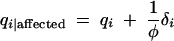
The connection between phenotype and marker genotypes can be determined by examining the “effect” of the marker genotype. For a discrete trait, this is the probability of being affected conditional on the marker genotype, P_affected|ij. This depends on the distribution of A_rA_s genotypes within M_iM_j genotype categories, which in turn depends on LD between the loci (D_ri),

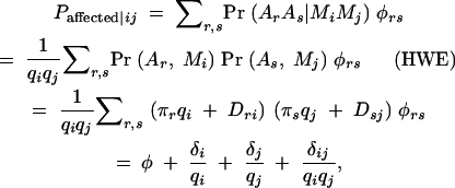2

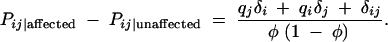
where the terms 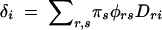and 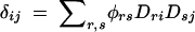. These terms are very convenient measures of association. For example, in the usual allele-based case-control test, marker allele frequencies among affected individuals, q_i|affected, are compared to their frequencies among unaffected individuals, q_i|unaffected,

3

4

so that

5

In the TDT, the proportion of times that marker allele M_i is transmitted to an affected offspring (T_i.) is contrasted with the proportion of times that it is not transmitted (T_.i). The expected difference between transmission and nontransmission rates is

where c is the recombination rate between loci. It is clear that as the recombination rate approaches 50%, this difference will become zero, implying this is also a test of linkage.

It is clear that both these tests of association depend on LD through the association measure δ_i. The penetrances of the genotypes at the genes are confounded with LD in this measure. The story is, in fact, more interesting than this. Applying a classical quantitative genetics model where the genetic effect of genotype, G_rs, is decomposed into additive effects (α_r) and dominance deviations (d_rs), G_rs can be written as

The least-squares solutions for the additive effects are α_r = ∑_sπ_sG_rs − μ (Weir and Cockerham 1977). In the case of penetrances, G_rs = φ_rs and μ = φ. Noting that ∑_rD_ri= 0,

This shows that it is a very specific genetic effect that is captured by these tests of association; it is the sum of the additive effects of the alleles at the gene (α_r), weighted by the D_ri terms. When considering susceptibility as the trait of interest, the additive effects of the susceptibility alleles represent Pr(affected|A_r) − φ (the effect of the allele A_r centered around the overall prevalence of the disease). Additionally, the additive effect of marker allele M_i is Pr(affected|M_i) − φ, which is δ_i/q_i. Both the allele-based case-control test and the TDT examine marker alleles individually rather than as whole genotypes, whereas it is whole genotypes that affect the phenotype. Therefore it is not surprising that these tests are capturing only the additive effects of the gene via the additive effects of the marker. That tests of association depend on this combined measure, δ_i, is intuitively appealing, as it shows that the strength of the effect of a marker allele on susceptibility depends on how strongly that marker allele is connected with each of the alleles at the gene, combined with how strongly those alleles themselves affect phenotype.

It is possible to capture nonadditive genetic effects (the dominance deviations, d_rs) by performing a genotype-based case-control test. Here marker genotype frequencies are contrasted between affected and unaffected individuals:

This contrast results in a linear combination of the individual allele association measures and the genotype association measure .

These results also extend to marker haplotypes (Nielsen and Weir 2001). Consider a second marker, N, with alleles N_k at population frequencies p_k. In addition to the pairwise LD terms between each marker and the gene, there is also pairwise LD between the markers, plus the three-locus LD term, D_kri (Equation 1).

A straightforward haplotype association test is the haplotype-based case-control test, in which haplotype frequencies among affected individuals are contrasted with those among unaffected individuals. These two-locus marker haplotype frequencies can be calculated as

6

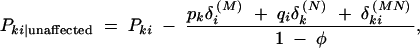7

where we have distinguished δ measures for each marker with a superscript. The marker haplotype measure δ^MN_ki is 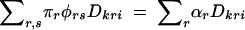. The difference between marker haplotype frequencies among cases and controls is

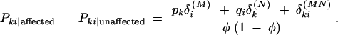8

By rearranging terms slightly, the factor δ^M_i/q_i + δ^N_k/p_k + δ^MN_ki/q_ip_k emerges, showing that this difference depends on the sum of the additive effects of marker alleles N_k and M_i plus a contribution from the additive effect of the joint N_kM_i haplotype. As each of the single-marker and haplotype association measures can be positive or negative, the combined haplotype measure might be less than the sum of its parts, rather than greater.

LD contrast test:

It is expected that both haplotype and allele frequencies differ between affected and unaffected individuals when the markers being examined are in LD with a gene affecting phenotype. Because of this, pairwise LD between the markers should also differ between affected and unaffected individuals. We can write out these LD coefficients using Equations 3, 4, 6, and 7.

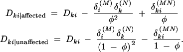This can provide the basis for a novel haplotype-based association test. The contrast between these measures is

For a sample size of N individuals, we can derive a test statistic based on this contrast using the following form:

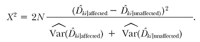9

We derive the variances for LD among cases and controls using the appropriate terms in the general form

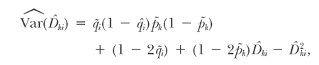where p̃ is the allele frequency estimator (Weir 1996). This test has an asymptotic chi-square distribution with (K − 1) × (I − 1) d.f., where K and I are the numbers of alleles at the markers. This test is sensitive to the same association terms as the haplotype-based case-control test (Equation 8), but in different combinations. This implies that these tests are sensitive to different patterns of LD. In addition, this LD contrast test has fewer degrees of freedom than the haplotype-based case-control test, which has up to K × I − 1 d.f. For example, if both markers are diallelic, there can be up to 3 d.f. for the case-control test (number of haplotypes minus one), whereas there is only 1 d.f. for the LD contrast test, as there is only one LD coefficient when examining two diallelic markers. To determine which test can perform better in which situations, it is important to understand the pattern of three-locus LD in addition to the pairwise measures. We have investigated this question through several types of simulation procedures.

Simulations:

We performed a number of simulations as part of our studies to understand the relationship between patterns of two- and three-locus LD and three tests of association. These tests included the single-marker case-control test, the haplotype-based case-control test, and the LD contrast test (described above). The basis of the simulations involved creating a large number of sets of three polymorphic loci, including two neutral markers and one functional site. Each of these sets of three loci differed from one another by their haplotype frequencies and therefore by their two- and three-locus LD patterns. To reduce the overall number of parameters involved, we assumed two diallelic markers (M and N) and a diallelic functional site (A). In this case there is one free LD coefficient for each pair of loci and one free three-locus LD coefficient for the set of three loci. There are up to eight possible three-locus haplotypes. We focused on three loci at a time for our simulations, as more loci would necessitate the incorporation of yet higher-order LD terms.

The power calculations were performed by applying a genetic model to the functional site for a group of three loci, with penetrance parameters described in Table 1. We then used the genetic model and the haplotype frequencies to generate samples of affected individuals (cases) and unaffected individuals (controls), along with their genotypes and haplotypes at the two neutral markers for each three-locus set. This was done by generating individual genotypes separately for cases and controls from the appropriate multinomial distributions with probabilities of the genotypes conditional upon affection status calculated using Bayes' rule and assuming random union of gametes for the unconditional genotype frequencies (P[A_rA_s] = P[A_r]P[A_s]). For each set of three loci, we created samples of 200 cases and 200 controls and performed the two single-marker case-control tests, the haplotype-based case-control test, and the LD contrast test. Haplotype phase was considered known rather than estimated. The sampling and testing procedure was repeated 10,000 times for each set of loci, and the proportion of times a given test rejected the null hypothesis of no association was recorded. This provided us with an estimate of the power of these tests under the conditions of each set of three loci.

TABLE 1.

Penetrances for the simulated genetic model

		φrs
Genotype	Frequency	Model 1	Model 2	Null model
A1A1	0.01	0.09	0.23	0.06
A1A2	0.18	0.06	0.13	0.06
A2A2	0.81	0.03	0.03	0.06

Each of the genetic models examined was additive; we were not concerned with nonadditive effects, as the allele-based tests we examined are sensitive to these effects only through the variances of the test statistics, and these effects are not substantial. We chose at least one reasonably low-penetrance model, simulating a gene with small marginal effects on overall susceptibility. The minor allele of the functional site was the one associated with higher risk. We made no assumptions regarding the relative positions of the three loci, as this information does not contribute to the tests other than through the LD terms.

Both two- and three-locus LD contribute to the power of a haplotype-based association test, whereas only two-locus LD affects single-marker tests. The relationship between each of the LD coefficients and the power of these tests, however, is not transparent (Equations 5 and 8). We were interested in examining what type of LD patterns cause haplotype-based tests to be more powerful than single-marker tests. We investigated this through simulation by contrasting estimates of the power of these tests under a large number of different combinations of values for the various LD terms.

For three diallelic loci, there are three pairwise LD terms and one three-locus term. Fully informative notation to distinguish these terms should include a component describing which loci and which alleles are being referred to (M_i, N_k, or A_r). For notational ease, we restrict ourselves to the use of subscripts, so that D_kr is LD between alleles N_k and A_r, and so forth.

Simulations based on real data:

We were interested in examining the types of LD patterns expected to be seen in real data as part of our study. To do this, we used three-locus estimates of haplotype frequencies from the data described in Zaykin et al. (2002). In their experiment, 138 individuals were genotyped for 552 SNPs on chromosome 12. These SNPs were divided into six regions containing ∼92 SNPs each. All possible three-SNP combinations were examined within each region, and three-locus haplotypes were estimated using an EM algorithm.

We incorporated this chromosome 12 information into our simulation procedure by using the three-locus haplotype frequency estimates as the basis for our sampling distribution. So, while the input values are estimates derived from real data, for our purposes here, we considered them to be the true population parameters of our simulations. This gave us an empirical distribution of the range of possible haplotype frequencies. As described above, each set contained two neutral markers (M and N) and one functional site (A). The allele frequency distribution for ascertained SNPs tends to be biased toward more common variants (Phillips et al. 2003). To attempt to counter this effect to some degree, the SNP with the smallest minor allele frequency was chosen to be the functional polymorphism for each three-locus set. The genetic models used for the functional site are described in Table 1, with the rarer SNP allele chosen to be the allele associated with higher susceptibility.

To reduce the number of three-locus sets that were considered, we used only loci that were within 50 SNPs of each other. We also did not include SNPs with minor allele frequencies <3%. This provided us with 206,975 three-locus combinations.

Iterative simulations:

The simulations based on real data provided an enormous number and range of combinations of LD patterns, making statements based on pattern types difficult. To make observations regarding how individual patterns of LD affect the power of these tests, we created a more systematic set of LD patterns using an iterative simulation approach. This was done by creating three-locus sets that covered the range of possible values for each of the LD terms. As before, for each three-locus set, we assign one locus to be functional and the other two to be neutral. Marker M had a minor allele frequency of 30% and marker N had a minor allele frequency of 20%. The minor allele frequency of the functional site, A, was 10%. The genetic models used for the functional site were the same as the simulations based on real data (Table 1).

To generate the combinations of values for the various LD terms, we used a nested loop, iterating from the largest (in absolute value) negative value possible for each LD term to the largest positive value. While the pairwise LD measures are restricted by the allele frequencies, the three-locus term is restricted by the two-locus haplotype frequencies. Because of this, we set the values of the three-locus LD measure in the innermost loop. The possible range for this parameter is often quite small, especially when the pairwise values were set to their extremes. In this case, possibly only one or no iteration of the final loop occurs. There were 6586 unique three-locus sets generated using this algorithm.

Corrections for multiple tests:

To make the comparisons between the single-marker and haplotype-based tests, we wanted to consider the effects of multiple testing, as there are two single-marker tests for each haplotype-based test performed. One possibility for doing this would be to use a Bonferroni correction to adjust the threshold for each single-marker test. This method, however, is conservative, especially when the tests are correlated. Another possible correction strategy could be to use a permutation method; however, with the number of simulations being performed and the computational burden required, this was not feasible. We were interested in determining a correction strategy that accounted for the correlation between tests due to LD between the markers and used the data directly.

We wanted to maintain the global type I error rate, the probability of any test falsely rejecting the null hypothesis, at 5%. In our case, we were interested only in the two tests performed for each experiment, so that the probability of any test falsely rejecting the null hypothesis is the probability that at least one of the two tests rejects. This probability is P_g = Pr(test 1 rejects) + Pr(test 2 rejects) − Pr(both tests reject) = α₁ + α₂ − P_joint. To maintain this at 5%, we estimated the uncontrolled global type I error rate, P_g(unadj) = 2α_unadj − P_joint(unadj) and then calculated the factor W such that P_g(unadj)/W = 0.05. The factor W could then be used to calculate the reduced level for each individual test as α_adj = 0.05/W. To allow the general use of this method, we needed an efficient way to estimate W. Noting that α_unadj is a fixed constant (in our case 0.05), the unknown component of P_g(unadj) is P_joint(unadj). We were interested in deriving a function that could be used to predict this probability on the basis of the level of LD between the markers, P_g(unadj) = f(r²), where

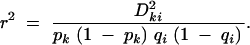10

To do this, we simulated data under the null hypothesis of no association between the phenotype and the markers and then performed 10,000 replications of unadjusted tests, tracking the frequency with which both tests simultaneously rejected the true null hypothesis and the level of LD between the markers. Conditions under the null hypothesis were simulated by setting the penetrance values for each “functional” genotype to the same value of 0.06 (Table 1). These simulations were performed using a subset of the data (one of the six regions from the chromosome 12 data, comprising 35,730 three-locus combinations, were used). In this manner, the three loci involved (the two markers and the putative functional site) were still dependent on each other through LD, but the phenotype was independent of all genotypes; P_affected|rs = P_affected = 0.06. A function predicting P_joint(unadj) from LD, f(r²), was empirically fit using the data points from these simulations. This function was then used to estimate W in simulations under the null hypothesis using the remaining five regions of the chromosome 12 data. As the second set of data had not been used for the derivation of f(r²), it served as a validation case to verify that P_g derived using the estimated factor W was indeed 0.05. The adjusted levels for these results were very close to the desired 0.05 level. This indicated that our multiple-correction method was effective for all LD combinations seen in this study and should be of general applicability.

Plotting P_joint vs. r² did provide useful information for determining an adjusted α level, but we wanted to gain a fuller understanding of the connection between correlations between the two tests and LD. To do this, we considered the binomially distributed variables T₁ (test 1 rejected or did not reject the null hypothesis of no association) and T₂ (test 2 rejected or did not reject). The correlation between these variables was calculated using the equation for correlation between binomial random variables: P_jointunadj− α²_unadj²/α²_unadj1 − α_unadj² (where, as before, α_unadj represents the unadjusted probability that either single-marker test rejects the null hypothesis [0.05] and P_joint(unadj) is the probability that they both reject the null hypothesis). By plotting these correlations between the two tests vs. LD (r²), we find a tight connection between the correlation of the tests and LD, although this connection is not linear (Figure 1). One interesting thing to note about Figure 1 is that LD must get quite high before correlation between the tests becomes substantial. Correlation between the tests reached ∼0.3 only when r² = 0.8.

Figure 1.—

Correlation between single-marker tests and LD. The correlation between two single-marker tests rejecting the null hypothesis of no association (along the y-axis) plotted as a function of the LD between the tests (along the x-axis) is shown. LD is measured as r² (Equation 10). The line shows the empirically fitted function that was used to predict correlation between the tests on the basis of LD between the markers.

RESULTS

For each three-locus set considered, the single-marker case-control tests, the haplotype-based case-control test, and the LD-contrast test were performed on 10,000 replicate samples and the power of each test was recorded and compared. We adjusted for the fact that two single-marker tests were performed by using the procedure described above, estimating W by the function f(r̂²), and then using it to adjust the critical levels. For comparison, we also recorded the results for the same simulations using a Bonferroni correction. There were two strategies for determining the input values for the two- and three-locus LD parameters for these locus sets. One strategy involved using LD patterns derived from haplotype frequency estimates from real data (Zaykin et al. 2002). The other strategy involved iterating through the range of possible values, maintaining constant single-marker allele frequencies. Using the results of these simulations, the single-marker tests and the two haplotype-based tests could be compared under a number of different combinations of two- and three-locus LD, and the results could be examined in various ways.

An overall summary of the results of the test comparisons for the simulations based on real data is given in Figure 2. Of all three-locus sets considered, the proportion of sets for which a given test was the most powerful, by at least τ%, is shown, where τ was set to 2, 5, or 10%. A tie was declared if the top two tests were within τ% of each other. The test with the highest power had to achieve at least 40% power to be considered successful. The category denoted “none” included those sets for which no test achieved ≥40% power. For penetrance model 1 (the one with weaker marginal effects) it can be seen that for >60% of the locus sets examined, none of the tests achieves ≥40% power. If the power of a test does exceed 40%, in a majority of cases it is a single-marker-based test that wins, although almost all the results are within 10% of each other. For penetrance model 2 (the model with reasonably large marginal effects), in a majority of cases, at least one test achieves ≥40% power. For this model, there is no substantial difference between the proportion of times each test is most powerful. As with the other model, in almost all cases, the power estimates of these tests are within 10% of each other.

Figure 2.—

Proportion of trials for which each test was most powerful. The proportion of three-locus sets for which a given test was the most powerful by at least τ%, where τ was set to 2, 5, or 10%, is shown. A tie was declared if the top two tests were within τ% of each other. The test with the highest power had to achieve at least 40% power to be considered successful. The category denoted “none” included those sets for which no test achieved ≥40% power.

The Bonferroni correction for the single-marker tests caused a reduction in the power of these tests relative to the haplotype-based case-control tests, as expected. The drop was not particularly large on average, however. For penetrance model 1 (smaller effects), there was an ∼3% loss in power of these tests. The loss was ∼2% for model 2.

Power across the chromosome 12 region:

A closer view of the relationship between LD patterns and the association tests can be gained by examining the results along the chromosomal region. This allows us to investigate both the relationship between LD patterns and power and whether the strategy of summarizing average LD along a chromosome is useful when planning an association-testing strategy. From this, we can also examine whether concurrently investigating both pairwise and three-locus LD can improve the selection criteria.

Dawson et al. (2002) examined average pairwise LD in moving windows along a chromosome. This gave a picture of average levels of LD along the chromosome. We performed a similar type of experiment using the results of the simulations based on real data. There were 552 SNPs examined in the chromosome 12 region described in Zaykin et al. (2002). We used the 490 of these with minor allele frequencies >3%. In our full set of simulations, we considered all combinations of three SNPs for which the SNPs were within 50 loci of one another. For each set of three SNPs, the one with the smallest minor allele frequency was considered functional for that set. We reduced the number of sets examined for the experiments described here. Only those sets for which the neutral markers were within 10 SNPs of the one chosen to be functional for that set were kept. All locus sets for which the rth SNP (S_r) was functional were then grouped together into the category G_r (r = 1–490). (For example, if S₂₅ was the functional SNP for each of the sets {S₁₇, S₂₅, S₂₈}, {S₂₅, S₂₆, S₂₉}, and {S₂₅, S₂₉, S₃₀}, these three sets would make up the category G₂₅.) The average power of a test _r to detect an association when S_r was functional by examining nearby SNPs (not including S_r) for each of the three tests performed was calculated as

11

where n_r is the number of three-locus sets in G_r. We could then plot _r for each type of test (single-marker case-control, haplotype case-control, and LD contrast) across the region of S_r SNPs. To eliminate some noise, a rolling average of the _r values is plotted, using a sliding window of five loci. Figure 3 shows a summary of the results. Figure 3, A and C, shows the rolling average of the power of the single-marker and haplotype-based case-control tests for penetrance models 1 and 3, respectively. The solid line designates the power of the haplotype test, and the shaded line denotes the single-marker tests.

Figure 3.—

Summary results for power comparisons along the chromosome. The horizontal axes represent the relative positions of the chromosome 12 SNPs (Zaykin et al. 2002, map not to scale). (A) Rolling averages for the power of the single-marker case-control tests (shaded line) and the haplotype-based case-control test (solid line) under penetrance model 1 (small effects). (B) Each point represents the difference between the power of the single-marker case-control test and that of the most powerful haplotype test under penetrance model 1 (see text for details). (C) Rolling averages as in A, but under penetrance model 2 (larger effects). (D) Differences in power as in A, but under penetrance model 2. (E) Rolling averages of pairwise (solid line) and three-locus (shaded line) LD along the chromosome. The scale of these values is given along the axis to the right.

More detailed information is shown regarding the comparisons of the single-marker tests with the haplotype tests in the scatterplots in Figure 3, B and D. There are n_r points plotted at position S_r. Each point represents the difference between the power of the single-marker tests minus the larger of the two haplotype-based tests. Thus, positive values indicate results in which the single-marker tests were more powerful, and negative values indicate that one of the haplotype tests was most powerful.

At the bottom of Figure 4E is a plot of average absolute value pairwise LD (solid line) and average absolute value three-locus LD (shaded line) vs. chromosomal location. The value of the pairwise measure at any point S_r along the chromosomal region is the rolling average of the terms

where H_r contains all two-locus pairs that included S_r as a functional SNP (a collapsing of G_r above). As we considered all triples for which the neutral markers were within 10 SNPs in either direction of the one chosen to be functional, m_r has an upper bound of 20. The rolling average is again taken with a sliding window of size five. The three-locus LD average includes values from all three-locus sets containing S_r as the functional site (G_r). These averages are calculated in the same manner as average power (Equation 11), above.

Figure 4.—

Power results for a subset of the iterative simulations. Power results for the three tests (single-marker case-control, haplotype-based case-control, and LD contrast) under different LD patterns for penetrance model 2 are shown. A includes all results for which pairwise LD between the markers and the functional site are low (D_kr = 0 and D_ir = 0.01). B displays results for stronger LD (D_kr = 0.02 and D_ir = 0.04). The bottom parts of A and B show the combination of three-locus LD and pairwise LD between the two neutral markers for each point along the power curve at the top. The values of pairwise LD between the markers have been scaled by a factor of ¹/₂₀.

From these results, a number of things can be seen. As was shown in Figure 2, in a majority of cases, the power of the haplotype-based case-control tests was within 10% of the power of the single-marker-based tests. When the haplotype-based test did outperform the single-marker test, however, it could be by a very large amount, especially for penetrance model 2 (Figure 3C, stronger effects). These cases where the haplotype tests have substantial power influence the average power of the haplotype-based tests. For penetrance model 2, this increase in average power was sufficient to make the average power for the haplotype-based tests larger than the average power for the single-marker tests (in spite of the fact that the single-marker tests won more frequently).

For penetrance model 1 (Figure 3A, weaker effects), there is a slightly larger tendency for the single-marker tests to win, and the differences in power are not quite as pronounced. Because of this, the average power for the single-marker tests appears to be slightly higher than the average power of the haplotype-based test. Both types of tests had very good power in regions where LD was high; these were the regions in which the tests tended to perform equally well. The LD contrast test showed lower power than the other two tests on average. There were cases, however, in which this test was the most powerful. The cases for which the power of the LD contrast test was at least 10% greater than either of the other two tests are marked by points at the bottom of the power curves in Figure 3, A and C. These cases appear to occur when both two-locus and three-locus LD are reasonably small and the power of the other tests is quite low.

One factor that may affect these results, particularly as presented in Figure 3, is whether we have chromosomal regions for which the minor allele frequencies are generally large (relative to the rest of the region). This could affect both the amount of LD present and the magnitude of the effect of the functional alleles, inflating the power in that region. We investigated whether this was the case in our data by examining the minor allele frequencies of the three loci across the chromosomal region. The results indicated that there were no trends or aggregates of similar allele frequencies in this region, so that this would not be a concern.

Effects of specific patterns of LD on power:

As the number and range of LD patterns seen in the real data were very large, it was not feasible to use these results to make comparisons between individual patterns and power. We used the results of the more systematic iterative simulations to determine these relationships directly, rather than through averaged results. Figure 4 shows an illustrative subset of the results of these simulations under penetrance model 2. Figure 4A shows the power results when pairwise LD between the markers and the functional site are small: D_kr = 0 and D_ri = 0.01 . The results shown in Figure 4B reflect higher pairwise LD between the markers and the functional site: and . In the bottom sections of Figure 4, A and B, all levels of three-locus LD and all levels of pairwise LD between the two neutral markers are displayed. Three-locus LD is shown by the solid dots. Pairwise LD values between the markers, shaded dots, are scaled by a factor of ¹/₂₀ so that they would fit within the bounds of the figure.

The power of the single-marker tests can be seen to rely on pairwise LD with the functional site, as would be expected. In Figure 4A, this power is low, whereas in Figure 4B, it is high. The interesting thing is how power of these tests compares with that of the haplotype-based tests. In general, the single-marker tests become the predominantly most powerful tests as the pairwise LD values between the markers and the functional site become large in absolute value. For less extreme values of the pairwise LD terms, the most powerful test tends to alternate between a single-marker test and the haplotype-based case-control test, although any of the three tests may come up as the most powerful. The haplotype-based tests were consistently more powerful when the three-locus LD was at its extremes, irrespective of the level of the pairwise LD terms. The most powerful test in this case alternated between the two haplotype-based tests. When the pairwise LD values drop to zero, even with moderate levels of three-locus LD, it is likely that none of the tests have power, but the only tests that have any possibility of detecting association are the haplotype-based tests.

The peaks in the graph represent changes in power due to pairwise LD between the two neutral markers. The effect of this LD term on the power of the haplotype tests is illustrated in Figure 5, which displays the results of the haplotype case-control test for D_kr = 0.02 and D_ri = 0.04 (as in Figure 4B). The solid circles are the results when three-locus LD are negative (D_kri = −0.006) and the open circles are when these values are positive (D_kri = 0.004). In the first case, power drops as pairwise LD between the neutral markers increases from negative to positive, while in the second case, the reverse occurs. This is unfortunate, as it indicates that predicting haplotype power by examining LD between the markers alone may not be possible.

Figure 5.—

Power results for the haplotype-based case-control test under penetrance model 2 when D_kr = 0.02 and D_ir = 0.04 (LD between the markers and the functional site) are shown. Solid circles are for negative three-locus LD (D_kri = −0.006) and open circles are for positive three-locus LD (D_kri = 0.004).

The LD patterns generated in this manner represent the range of possible combinations of the four LD terms, given the allele frequencies considered. It is possible that some of these combinations are unlikely to occur in real data. To examine this question, we extracted a subset of the real data for which the allele frequencies were similar to the simulated frequencies. In this subset of the real data, we saw a large range of two- and three-locus LD patterns, which included the spectrum of possible two-locus and three-locus LD terms. While this does not provide a rigorous examination of the likelihood space of two- and three-locus LD patterns, it does indicate that individual patterns should not be excluded from consideration, although they may be less common than others.

DISCUSSION

We examined several questions regarding patterns of two- and three-locus LD and the power of single-marker and haplotype-based tests of association. We addressed these questions through two types of simulations. One simulation strategy involved using haplotype patterns estimated from real data (Zaykin et al. 2002). This provided us with an empirical distribution of LD patterns. It also provided a framework for examining whether strategies for testing for association can be derived by utilizing LD summaries (such as those of Dawson et al. 2002). The other simulation strategy involved iterating over a wide range of LD patterns with fixed allele frequencies. These simulations were designed so that relationships between LD patterns and the various types of tests could be determined.

A general conclusion is that each of the tests studied here has its merits. While it is possible that in many situations all three tests have similar power to detect association, so that single-marker tests can be effectively used and the haplotype-based tests disregarded, in a reasonable proportion of situations this is not the case. When the haplotype-based tests were more powerful, it could be by a very large degree. If single-marker tests are to be used, it does appear that a multiple-testing adjustment that takes LD between the markers into consideration should be applied, as the Bonferroni correction can reduce power. Our method is effective for jointly testing two SNPs. A permutation method can also be applied for two or more SNPs.

There are patterns of LD for which one of the haplotype-based tests appears to be best suited. For instance, if pairwise LD values between the markers and the functional site are close to zero, the only hope for detecting association appears to be the LD-contrast test, as this test appears to be the most sensitive to smaller values of the three-locus LD term. Displaying the power results along the chromosome (Figure 3) gives an indication of the regions for which it will be difficult or easier to locate SNPs associated with the phenotype. These results are closely related to the patterns of two- and three-locus LD across the chromosome (Figure 3E), showing that maps such as these may be useful in predicting power to detect associations.

One important consideration when interpreting the results based on real data is that the properties imposed on the sites considered to be functional, such as the allele frequency distribution and the levels of LD with surrounding markers, were dictated by the properties of those SNPs ascertained in the samples described in Zaykin et al. (2002). It is reasonable to assume that the properties of true functional sites are not the same as the properties of SNPs ascertained for association studies. For common variants, however, it seems reasonable that these results should be realistic.

Both of these simulation procedures were performed assuming that all three loci involved are diallelic. In the case of a multiallelic functional site, the relationship between LD and marker/phenotype association becomes much more complicated. In this case the results from comparing the different types of tests may be quite different and are a topic for further study.

References

- Akey, J., L. Jin and M. Xiong, 2000. Haplotypes vs single marker linkage disequilibrium tests: What do we gain? Eur. J. Hum. Genet. 9: 291–300. [DOI] [PubMed] [Google Scholar]
- Ardlie, K. G., L. Kruglyak and M. Seielstad, 2002. Patterns of linkage disequilbrium in the human genome. Nat. Rev. Genet. 3: 299–309. [DOI] [PubMed] [Google Scholar]
- Bennett, J. H., 1954. On the theory of random mating. Ann. Eugen. 18: 311–317. [DOI] [PubMed] [Google Scholar]
- Brouwer, D. A., J. J. van Doormaal and F. A. Muskiet, 1996. Clinical chemistry of common apolipoprotein e isoforms. J. Chromatogr. B Biomed. Appl. 678: 23–41. [DOI] [PubMed] [Google Scholar]
- Dawson, E., G. R. Abecasis, S. Bumpstead, Y. Chen, S. Hunt et al., 2002. A first-generation linkage disequilibrium map of human chromosome 22. Nature 418: 544–548. [DOI] [PubMed] [Google Scholar]
- Fallin, D., A. Cohen, L. Essioux, I. Chumakov, M. Blumenfeld et al., 2001. Genetic analysis of case/control data using estimated haplotype frequencies: application to APOE locus variation and Alzheimer's disease. Genome Res. 11: 143–151. [DOI] [PMC free article] [PubMed] [Google Scholar]
- Hill, W. G., 1976 Non-random association of neutral linked genes in finite populations, pp. 339–376 in Population Genetics and Ecology, edited by S. Karlin and E. Nevo. Academic Press, New York.
- Kaplan, N., and R. Morris, 2001. Issues concerning association studies for fine mapping a susceptibility gene for a complex gene. Genet. Epidemiol. 20: 432–457. [DOI] [PubMed] [Google Scholar]
- Long, A. D., and C. H. Langley, 1999. The power of association studies to detect the contribution of candidate genetic loci to variation in complex traits. Genome Res. 9: 720–731. [PMC free article] [PubMed] [Google Scholar]
- Nielsen, D. M., and B. S. Weir, 1999. A classical setting for associations between markers and loci affecting quantitative traits. Genet. Res. 74: 271–277. [DOI] [PubMed] [Google Scholar]
- Nielsen, D. M., and B. S. Weir, 2001. Association studies under general disease models. Theor. Popul. Biol. 60(3): 253–263. [DOI] [PubMed] [Google Scholar]
- Phillips, M. S., R. Lawrence, R. Sachidanandam, A. P. Morris, D. J. Balding et al., 2003. Chromosome-wide distribution of haplotype blocks and the role of recombination hot spots. Nat. Genet. 33(3): 382–387. [DOI] [PubMed] [Google Scholar]
- Spielman, R. S., R. E. McGinnis and W. J. Ewens, 1993. Transmission test for linkage disequilibrium: the insulin gene region and insulin-dependent diabetes mellitus (IDDM). Am. J. Hum. Genet. 52: 506–516. [PMC free article] [PubMed] [Google Scholar]
- Thomson, G., and M. Baur, 1984. Third order linkage disequilibrium. Tissue Antigens 24: 250–255. [DOI] [PubMed] [Google Scholar]
- Thomson, G., and W. Bodmer, 1979. HLA haplotype association with disease. Tissue Antigens 13: 91–102. [DOI] [PubMed] [Google Scholar]
- Wall, J. D., and J. K. Pritchard, 2003. Haplotype blocks and linkage disequilibrium in the human genome. Nat. Rev. Genet. 4(8): 587–597. [DOI] [PubMed] [Google Scholar]
- Weir, B. S., 1996 Genetic Data Analysis II. Sinauer Associates, Sunderland, MA.
- Weir, B. S., and C. C. Cockerham, 1977 Two-locus theory in quantitative genetics, pp. 247–269 in Proceedings of the International Conference on Quantitative Genetics, edited by E. Pollak, O. Kempthorne and T. B. Bailey. Iowa State University Press, Ames, IA.
- Zaykin, D. V., P. H. Westfall, S. S. Young, M. A. Karnoub, M. J. Wagner et al., 2002. Testing association of statistically inferred haplotypes with discrete and continuous traits in samples of unrelated individuals. Hum. Hered. 53: 79–91. [DOI] [PubMed] [Google Scholar]