Genetic Variation for Total Fitness in Drosophila melanogaster

Abstract

The extent of genetic variation in fitness is a crucial issue in evolutionary biology and yet remains largely unresolved. In Drosophila melanogaster, we have devised a method that allows the net effects on fitness of heterozygous wild-type chromosomes to be measured, by competing them against two different “balancer” chromosomes. We have applied the method to a large sample of 40 wild-type third chromosomes and have measured fitnesses of nonlethal chromosomes as well as chromosomes bearing recessive lethals. The measurements were made in the environment to which the population was adapted and did not involve inbreeding. The results show an extraordinary similarity in the behavior of replicates of the same chromosome, indicating consistent genetic effects on total fitness. Some invading chromosomes increased rapidly and some slowly, and some rose to appreciable frequency after several months, but then declined again: in every case, the same pattern was seen in each replicate. We estimated relative fitnesses, rates of change of fitness, and relative viabilities, for each chromosome. There were significant fluctuations around the fitted model, which were also highly replicable. Wild-type chromosomes varied substantially in their effects on heterozygous fitness, and these effects vary through time, most likely as a result of genotype × environment interactions.

FUNDAMENTAL features of the living world depend on the structure of fitness variation. Additive genetic variance in net fitness is the quantity that determines the rate at which populations adapt (Fisher 1930); females can evolve to prefer mates carrying “good genes” only if there is sufficient additive variance in fitness (Charlesworth 1987); life histories evolve according to the trade-offs between fitness components (Stearns 1992); and most random genetic drift may be caused by the hitchhiking effects of selection at linked loci (Gillespie 2001). It is thus of fundamental importance to understand the nature of genetic variation in net fitness and the contributions to it of different components of fitness.

Few studies have measured genetic variation for net fitness (Burt 1995). Observations of natural populations (e.g., Clutton Brock 1988; Kruuk et al. 2000; Merila and Sheldon 2000) are complicated by limited sample size and uncontrolled environmental variation. Laboratory experiments on microbes (e.g., Lenski and Travisano 1994) avoid these difficulties, but almost always use asexual populations, under conditions that are far from natural, and are based on new mutations rather than standing variation. In Drosophila, the overall fitness of heterozygous genotypes has rarely been measured (Curtsinger 1990; Fowler et al. 1997). Many studies have examined components of fitness (e.g., Mukai and Yamaguchi 1974; Mukai and Nagano 1983) or net fitness of homozygous genotypes (e.g., Sved 1971, 1975). Such studies are problematic, because there are often negative genetic correlations between different components of fitness (e.g., Partridge and Fowler 1992, 1993) and because homozygosity unmasks recessive alleles that would not be expressed in nature. Moreover, measurements of fitness have rarely been conducted under the conditions in which the life history evolved (Gibson et al. 2002); yet, fitness traits are often sensitive to gene × environment interaction (Kondrashov and Houle 1994; Gardner et al. 2001; Teotónio et al. 2002) and inbreeding may be induced by changed conditions (Teotónio et al. 2002).

Sved (1971)(1975) introduced a simple method for measuring the total fitness of homozygous wild-type chromosomes in Drosophila melanogaster. An advantage of this method over earlier studies is that it is possible to measure fitness under the environmental conditions and genetic background to which the chromosomes are adapted. Population cages containing a balancer chromosome (B) together with a wild-type chromosome (+) reach an equilibrium in which +/+ and B/+ genotypes segregate at frequencies reflecting their relative fitnesses. (Balancer chromosomes carry multiple inversions that suppress recombination, dominant visible markers, and recessive lethals; thus, B/B die, and B/+ are maintained by heterozygote advantage; homozygotes for whole wild-type chromosome are almost always substantially less fit than B/+.)

The Sved method suffers the disadvantage that it measures homozygous rather than heterozygous fitness. A novel method that is described in detail elsewhere (Fowler et al. 1997; Barton and Partridge 2000) measured variation in total heterozygous fitness by simultaneously competing wild-type chromosomes against two different balancer chromosomes. If fitnesses do not vary too much, then a polymorphic equilibrium can be reached, with all three balancers present. If wild-type homozygotes have zero fitness, then heterozygous fitnesses can then be estimated directly: the frequencies of the three heterozygous genotypes provide enough information to give their three fitnesses. (When wild-type homozygotes are viable and fertile, the Sved method can be used to provide the extra information needed to give all four fitnesses.)

When one balancer is much more fit than the other, there may be no stable polymorphism. Then, the temporal pattern of replacement of one balancer by the other (“invasion”) allows fitnesses to be estimated. Fowler et al. (1997) applied this method to 12 wild-type third chromosomes, extracted from a laboratory-adapted population, Dahomey. This stock has been held in population cages since 1970, with overlapping generations and at its carrying capacity. Fowler et al. (1997) found highly replicable differences in the pattern of invasion, which implied strong fitness differences. The fitness effects of wild-type chromosomes when combined with the two balancers were significantly correlated, but there were also significant differences between them. This implies that there are both additive and dominance components of fitness. Remarkably, there were significant fluctuations through time around the fitted model, which were correlated across replicates. This correlation between replicate cages implies strong genotype × environment interactions, such that particular wild-type chromosomes responded differently to environmental fluctuations experienced by the experimental cages.

We have now applied this method to 40 chromosomes from the same population. Our aims were: (i) to extend measurements to a larger sample of chromosomes; (ii) to measure fitnesses of nonlethal chromosomes, as well as of those bearing recessive lethals; and (iii) to measure components of fitness. In particular, we measured preadult viability both within the experiment and in a separate study (Gardner et al. 2001). The genetic correlations between the different components of fitness (including female fertility and longevity) and their contributions to total fitness variation will be reported separately.

The results of this study are qualitatively similar to those of the previous experiment, but are even more striking. All chromosomes show highly replicable patterns. In 21 invasion lines, the pattern was similar to that seen in the previous experiment, again with highly replicable patterns. However, 5 chromosomes never invaded, and for 14 wild-type chromosomes the invading chromosome began to increase, but then decreased again. As before, fluctuations around the fitted model were correlated across replicates, implying that subtle environmental variations have distinct effects on the fitnesses of different wild-type chromosomes. Such high replicability has been found elsewhere in large-scale, long-term selection experiments in D. melanogaster (Weber 1996; Curtsinger and Ming 1997). Thus, population cage experiments provide a way to measure fitness variation under seminatural conditions and open up the possibility of more detailed analysis—for example, of fitness components and of epistatic interactions. The results from this and from our previous experiment (Fowler et al. 1997) show remarkably high heritable fitness variation, of the kind required to explain key evolutionary phenomena such as hitchhiking and “genetic draft” (Gillespie 2001), the maintenance of sex and recombination, and the evolution of adaptive mate preferences.

METHODS

Population cages:

Except where stated, the experiment was performed in the same way as that in Fowler et al. (1997); additional details of culture conditions are given in Gardner et al. (2001). Balancer stocks were regularly backcrossed to the Dahomey base population and were maintained in very large numbers (several thousand) to ensure a diverse genetic background that differed little between lines. One hundred eighty wild-type third chromosomes were extracted from the Dahomey base population, of which 30 carried recessive lethals. This is similar to the frequency in nature (Simmons and Crow 1977) and the frequency in our previous extraction (30/150; Fowler et al. 1997). We chose to study all 30 lethal-bearing chromosomes, together with 10 nonlethal chromosomes.

We used the balancers TM1 and TM2, which carry multiple inversions that suppress recombination; TM1 is marked with Moiré eye (Me) and TM2 with Ultrabithorax (Ubx). For each replicate experimental chromosome (+_a, say), we set up two population cages of pure TM1/+_a genotype and two of TM2/+_a genotype. This replication controls for accumulation of new mutations on the + chromosome, for the effects of any recombination with the balancers, and for genetic drift. After allowing 63 days for these cages to reach their carrying capacity, we began the invasion by sampling eggs from each of the cages containing TM2/+. These samples were reared to adulthood, and 50 flies of each sex were introduced into each of the corresponding TM1/+ cages. These flies were introduced simultaneously into all 80 experimental cages. Following the introduction, samples of eggs were taken twice each week for ∼300 days. Our experiment differed slightly from that of Fowler et al. (1997) in that more flies were introduced at the start (100 vs. 40), subsequent sampling was less frequent (twice per week rather than three times), and somewhat fewer flies were counted (∼250, twice per week). The sampling scheme is improved by increasing the number of replicate cages rather than by increasing the number of flies counted (Barton and Partridge 2000). Overall, a similar number of flies was counted and classified by genotype: >1.2 × 10⁶ flies in each experiment. The positions of the experimental cages were randomized. There was no evidence of contamination since no wild-type flies invaded the experimental cages. (Note that if contaminants introduced a different wild-type chromosome, the wild-type would increase to fixation, since +_a/+_b does not suffer inbreeding depression.)

Estimates assuming constant fitnesses:

Fitnesses were estimated in the same way as in Fowler et al. (1997); theoretical issues are explored in more detail by Barton and Partridge (2000). A discrete-generation model was used to calculate the pattern of genotype frequencies through time. Thus, the probability of obtaining the observed samples could be calculated, given these frequencies, yielding the likelihood of the model. Hypotheses can be distinguished by comparing their likelihoods: in large samples, twice the difference in log likelihood is distributed as χ². In most cases, however, there is significant residual variation around the fitted models, such that the difference in log likelihood between the fitted model and a perfect fit is several times that expected under binomial sampling error. We allow for this excess error by treating the ratio between the difference in log likelihood between the hypotheses of interest and the residual difference in log likelihood as an F-statistic.

This discrete-generation model is an approximation to the actual age-structured population, which reproduces continuously in time. There is an inherent difficulty in reducing the many parameters of an age-structured model to a single fitness measure. However, Barton and Partridge (2000) show that age-structured models give patterns that are close to those of the best-fitting discrete approximation, and that the discrete-fitness estimates correspond to those required to fit the initial rate of increase of TM2, and decrease of TM1, in the invasions. As in Fowler et al. (1997), we assume a generation time of 15 days. Assuming a longer generation time would require larger fitness differences among genotypes to account for the same rates of change through time. In cases where wild-type homozygotes have zero viability, the basic discrete-time model has five parameters: the fitnesses of TM1/+ and TM2/+ relative to the standard TM1/TM2 genotype, the viabilities of TM1/+ and TM2/+ relative to TM1/TM2, and the initial frequency of TM2.

Relative viabilities are required to relate the observed frequencies of adults in the sample vials to the zygote frequencies; they can be estimated because when TM2 is rare, almost all flies are TM1/+, and so the two rare genotypes TM2/+ and TM1/TM2 must be at the same frequency in zygotes. (Nonrandom mating would need to be extremely strong for flies bearing TM2 to seek out mates with genotypes other than the predominant TM1/+.) Similarly, as TM1 is being eliminated, the two rare genotypes TM1/+ and TM1/TM2 must be equally frequent in zygotes. If adult +/+ homozygotes are observed in samples, then two more parameters are required: the viability and the fitness of +/+ relative to TM1/TM2.

The model assumes that relative fitnesses stay constant, in which case the parameter p₀ is the initial allele frequency. This depends on the number of adults introduced (100) relative to the number of larvae and pupae that will reach adulthood, as well as the number of adults in the cage, and so may be very low (Fowler et al. 1997). However, the transient appearance of TM2 in many cages implies that fitnesses can change. In that case, p₀ should be seen as a composite parameter that describes the delay before invasion of TM2 begins. That delay may vary by chance and also because of changes in relative fitness.

Roughly speaking, the rate at which TM2/+ displaces TM1/+ gives the relative fitness of those two heterozygous genotypes, while the time during which both balancers coexist gives an estimate of the fitness of the double-balancer genotype, TM1/TM2 relative to the two wild-type heterozygotes. With the large sample sizes used in this experiment, accurate estimates of both relative fitnesses can be made (see Barton and Partridge 2000, Figure 7). However, TM1/TM2 has very low fitness, and in some cases the best estimate is that this reference fitness is zero. In such cases, only the fitness of TM1/+ relative to TM2/+ can be estimated accurately. In cases where TM2 never becomes common, it is not possible to distinguish the fitnesses of TM2/+ from TM1/TM2, since the rate of change of TM2 depends only on the ratio (W_TM2/+ + W_TM1/TM2)/W_TM1/+ (for lethal or sterile +/+). This ratio will be close to W_TM2/+/W_TM1/+, since the double-balancer heterozygote has low fitness.

Estimates assuming varying fitnesses:

To account for the 14 “transient” cases where TM2 increases but then disappears, we must suppose that relative fitnesses change through the course of the experiment. We fit the simplest model that can account for the observations by assuming that the fitness of the common genotypes relative to the rare genotypes (i.e., W_TM1/+ and W_+/+ relative to W_TM2/+ and W_TM1/TM2) increases exponentially at a rate β per day. As discussed below, there is no evidence that the relative fitnesses of the two common genotypes change, and so we keep these fixed. However, there is no evidence as to the relative fitnesses of the two rare genotypes, since these must be at equal frequency in zygotes; our assumption here of fixed fitnesses of TM2/+ relative to TM1/TM2 is arbitrary. We assume that relative viabilities are fixed, since these were measured under standard conditions in sample vials (although see below). We assume an exponential change in fitness because our analysis is throughout in terms of log fitnesses, which thus change linearly at a rate β. Of course, more complicated patterns of fitness change could be fitted, but there is little power to distinguish them.

For the “transient” lines, we cannot estimate all the parameters of the model. In other words, the likelihood surface is flat in certain directions. We therefore multiply log likelihood by a penalty function, of the form Exp[−λ/v] for parameter v, with λ = 10⁻⁸. This ensures that a well-defined maximum exists, a little away from the boundary at v = 0. Maximization uses Mathematica's built-in Newton-Raphson algorithm. We have not seen evidence for multiple maxima in checks using different starting points. However, we have obtained somewhat better fits in regions where the likelihood surface is flat using our present algorithm than in the previous analysis (Fowler et al. 1997). Therefore, some of the values given in supplementary Tables S1 and S2 (http://www.genetics.org/supplemental/) for lines from Fowler et al.'s (1997) data differ slightly from the estimates in that article.

Deviations from the fitted models were examined using differences in arcsine-transformed genotype frequencies. The transformation was used, as in Fowler et al. (1997), so that variance due to sampling N individuals is 4/N. Residuals were plotted against either time or predicted TM2/+ frequency. Overall mean deviations, and correlations between replicate cages, were calculated by pooling residuals into bins 20 days wide or spanning ±10% predicted genotype frequency.

RESULTS

Patterns of invasion:

The 40 wild-type chromosomes fell into three classes (Table 1). In 5 cases, TM2 was never observed. In 16 cases, TM2 was not observed for a substantial time; in 13 of these, TM2 declined after rising to moderate frequency; while in the other 3, no decline was seen. However, in these 3 cases the increase occurred so late that the experiment ended before a decline would have been evident. In the remaining 19 cases, TM2 invaded and displaced TM1. We term these three classes “noninvader,” “transient,” and “invader,” respectively. There was no significant difference in pattern between wild-type chromosomes with and without recessive lethals . However, there are significantly fewer successful invasions by TM2 in this experiment compared with that in Fowler et al. (1997) (, P = 0.0067).

TABLE 1.

Classification of the 40 wild-type chromosomes in this experiment and the 12 in Fowleret al. (1997)

	TM2 never seen	TM2 transient	TM2 invaded	Total
+/+ viable	0	6	4	10
+/+ lethal	5	10	15	30
Fowler et al. (1997)	0	1	11	12

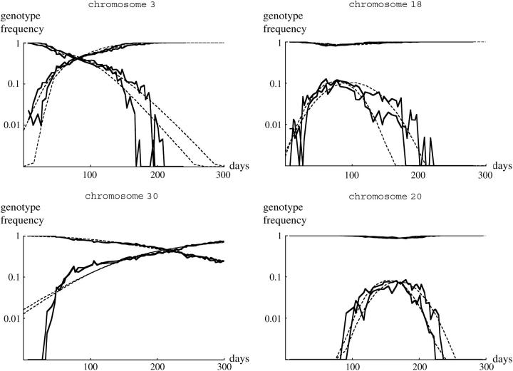
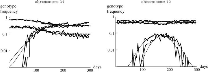
Remarkably, for all 40 pairs of cages the same class of pattern was seen across replicates. Moreover, detailed patterns were remarkably similar between replicate cages. For example, in both cages containing chromosome 18, TM2 was found in samples soon after its introduction, peaked at around 10% at day 80, and then declined (Figure 1). Replicates were similarly close for chromosomes that allowed TM2 to invade succesfully and where wild-type homozygotes were viable (Figure 1). For example, in cages containing chromosome 3, TM2 invaded quickly and became more common than TM1 after ∼70 days. TM2 also successfully invaded cages containing chromosome 30, but much more slowly, with TM2 becoming more common than TM1 only after 200 days. Moreover, both replicates showed a rapid increase in TM2 around day 50, followed by much slower change. The examples shown in Figure 1 are typical: for every chromosome, replicates showed close similarity, with appreciable differences occurring only when TM1 or TM2 is rare.

Figure 1.—

Examples of the changes in genotype frequency through the experiment. Three examples where TM2 invaded successfully are shown (left column), together with three examples where TM2 was seen only transiently (right column). The top two rows shows wild-type chromosomes that are recessive lethal, while the bottom row shows examples where +/+ are viable. Each part shows the increase in TM2/+ frequency and the decrease in TM1/+ frequency for each of the two replicate cages. (Except at low frequency, these are almost indistinguishable on this scale.) Where wild-type homozygotes are viable, their frequency is also shown; this is the bottom set of curves for chromosome 34 (bottom left) and the top set for chromosome 40 (bottom right). The pairs of dashed curves give the best-fitting theoretical prediction, separately for each replicate (supplementary Table S1, http://www.genetics.org/supplemental/).

The 10 pairs of cages for which wild-type homozygotes were viable showed similar patterns, in that TM2 either invaded and rose to high frequency (e.g., Figure 1, chromosome 34) or appeared transiently (e.g., Figure 1, chromosome 40). At the beginning of the experiment, there was a stable polymorphism with TM1/+ and +/+ present. In the six cases where TM2 never reached high frequency, this polymorphism was barely perturbed, indicating that the relative fitnesses of TM1/+ and +/+ remained constant throughout. In the other four cases, where TM2 rose to high frequency, the frequency of +/+ as well as TM1/+ decreased; this is to be expected if TM2/+ is more fit than TM1/+. Strikingly, however, in all these four cases a balanced polymorphism was reached, with TM1 apparently maintained at stable frequency at the end of the experiment (e.g., Figure 1, chromosome 34). Such a polymorphism was never seen when +/+ were lethal: in all those cases, either TM1 or TM2 was eliminated by the end of the experiment (e.g., Figure 1, chromosomes 3, 18, and 20). This pattern is surprising, because the conditions for polymorphism are more restrictive when wild-type homozygotes are viable and fertile:

1

(from Equation 4 of Barton and Partridge 2000). However, we will see that the estimated fitness of +/+ is so low that it has no appreciable effect on the population (Table S1).

Estimates assuming constant fitnesses:

We begin by fitting a model with constant fitnesses to those lines where TM2 invaded, as in Fowler et al. (1997). For chromosomes with +/+ lethal, this model has five parameters: p₀, the initial frequency of TM2; W_TM1/+, W_TM2/+, the fitnesses of TM1/+ and TM2/+ relative to TM1/TM2; and V_TM1/+, V_TM2/+, the egg-to-adult viabilities of those genotypes in sample vials, again relative to TM1/TM2. Where wild-type homozygotes are viable, there are two more parameters: the fitness and viability of +/+ relative to TM1/TM2. When TM2 is rare, TM2/+ and TM1/TM2 must be at the same frequency in zygotes, and so their relative viability can be measured from frequencies in emerging adults and similarly for TM1 rare. The estimates of relative fitness come primarily from the rate of increase of TM2 (λ_TM2 = (W_TM2/+ + W_TM1/TM2)/W_TM1/+ if W_+/+ = 0) and the rate of elimination of TM1 (λ_TM1 = (W_TM1/+ + W_TM1/TM2)/W_TM2/+ if W_+/+ = 0). The estimates for the invader lines, assuming constant fitnesses, are summarized in Table S1.

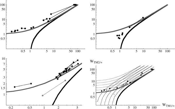
Figure 2 plots estimates of TM2/+ fitness against TM1/+ fitness, with pairs of replicates connected by lines. The +/+ lethal lines (top left) show remarkable agreement between replicates. Necessarily, all estimates lie above the top curve, which is the threshold for elimination of TM1 by TM2. Many estimates are clustered at top right; these correspond to very low fitness of the double-balancer genotype, TM1/TM2. For those lines where +/+ was viable, the estimated fitnesses of the heterozygous genotypes are quite different: they lie between the thresholds for invasion of TM2 and loss of TM1 (top right). This corresponds to the tendency of these lines to approach a balanced polymorphism, noted above. Again, we cannot see any statistical reason why these chromosome lines should differ systematically from those carrying recessive lethals. Fowler et al. (1997) found that in 11 of their 12 lines TM2 invaded and displaced TM1, while one line (denoted here as line 52) approached a polymorphism. Those fitness estimates follow the same relationship as do the invader lines in our experiment, but span a much narrower range of values of W_TM1/+ (compare top left and bottom left). The key finding here is that there are large and highly replicable fitness differences between genotypes carrying different + chromosomes.

Figure 2.—

Estimated fitnesses of TM2/+ and TM1/+, relative to TM1/TM2, for those cases where TM2 invaded successfully. These estimates are made assuming constant fitnesses. In each part, the top heavy curve shows the threshold for elimination of TM1, and the bottom heavy curve shows the threshold for invasion of TM2; thus, wild-type chromosomes with fitnesses between the two curves can remain polymorphic with both TM1 and TM2 present. Pairs of replicates are linked by lines. Top left, the 15 chromosomes for which +/+ was lethal. In six cases, the estimated TM1/TM2 fitness was extremely low. These are shown by pairs of circles superimposed at top right. Top right, the 4 chromosomes for which +/+ was viable. Bottom left, the 12 chromosomes from Fowler et al. (1997). (Note the narrower range of fitnesses.) The pair of shaded circles shows line 52, in which TM2 invaded but did not displace TM1. Bottom right, comparison between all three classes. For clarity, only the geometric means of replicate estimates are shown, so that pairs of points are replaced by a single point midway between. Solid circles, +/+ lethal; dark-shaded circles, from Fowler et al. (1997); light-shaded circles, +/+ viable. The dashed contours show the initial rate of increase of TM2 per generation (steeper curves) and the final rate of elimination of TM1 (shallower curves); contours are for increase by 10^0.2, 10^0.4, … 10 per generation.

Figure 2, bottom right, compares estimates for all three classes of chromosome; for simplicity, only the averages across replicates are shown. The differences among these classes can be seen clearly. This also shows contours for the rate of invasion of TM2 and the rate of loss of TM1. When TM1/TM2 is extremely unfit (top right), these rates both depend primarily on the fitness ratio W_TM1/+/W_TM2/+, so that the contours for invasion rates become parallel. Thus, it becomes impossible to estimate these fitnesses separately with any accuracy. This is reflected in the larger differences between replicates at upper right.

It is striking that the fitness estimates for those chromosomes carrying recessive lethals almost all lie just above the threshold for loss of TM1, but are widely scattered along it: in other words, the rate of loss of TM1 is similar across all lines, and fairly slow, whereas the fitness of TM1/+ relative to TM1/TM2 varies widely. We cannot see any reason why the estimates should not have been scattered over a wider region in the vertical direction: this would have corresponded to lines in which TM1 was lost more rapidly. There is a genuine pattern in which the rate of invasion of TM2 varies greatly against different wild-type chromosomes, but the rate of elimination of TM1 is more similar between chromosome lines and on average slower. [One might worry that these patterns arise from spurious correlations caused by sampling error: the distributions seen in Figure 2 might reflect covariation of the sampling errors in the two estimates of relative fitness. However, sampling error is expected to be quite small for the sample sizes used here (see Barton and Partridge 2000, Figure 7), as is confirmed by the good agreement between replicates seen in Figure 2.]

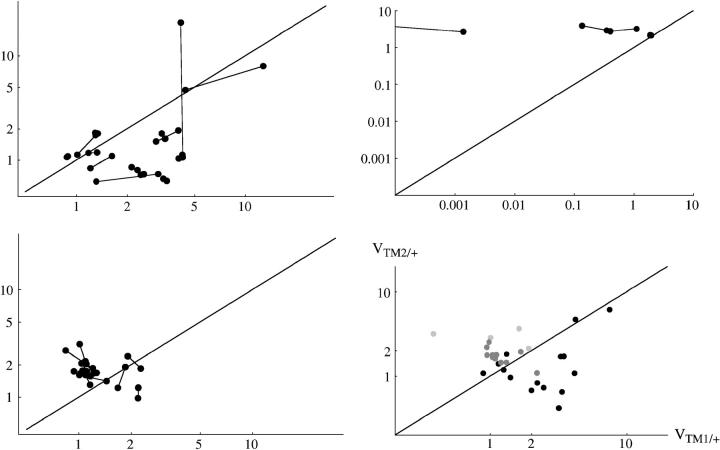
Figure 3 shows similar plots for the estimated viabilities. Again, there is good agreement between replicates. For TM1/+, Kendall's rank correlation between replicates is 0.71 (P < 10⁻³) for +/+ lethal and 0.345 (P = 7.7%) for the lines of Fowler et al. (1997). For TM2/+, the corresponding values are 0.70 (P < 10⁻³) and 0.27 (P = 12.5%). (Significance tests are based on 1000 randomizations across replicates. Values are not given for +/+ viable since there were only four such lines.) There are also differences between classes of chromosome: in this experiment, TM2/+ was in most cases less viable than TM1/+ for the +/+ lethal lines, but more viable than TM1/+ for the +/+ viable and for Fowler et al.'s lines. Moreover, viability estimates for Fowler et al. (1997) spanned a narrower range.

Figure 3.—

Estimated viabilities of TM2/+ and TM1/+, relative to TM1/TM2, for those cases where TM2 invaded successfully. These estimates are made assuming constant fitnesses (Table S1). Pairs of replicates are linked by lines. Top left, the 15 chromosomes for which +/+ was lethal. Top right, the 4 chromosomes for which +/+ was viable. (Note the very low viability of TM1/+ in one pair of replicates.) Bottom left, the 11 chromosomes from Fowler et al. (1997) in which TM2 invaded. (Line 52, in which TM2 did not fix, is not shown, because viability estimates there are confounded.) Bottom right, comparison among all three classes. Only the geometric means of replicate estimates are shown. Solid circles, +/+ lethal; dark-shaded circles, from Fowler et al. (1997); light-shaded circles, +/+ viable.

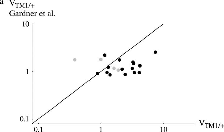
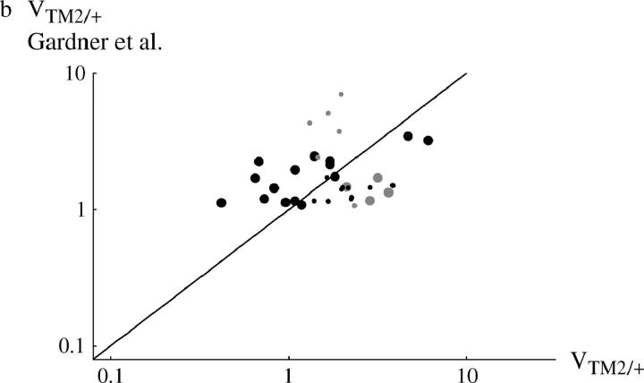
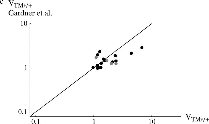
Figure 4 compares viability estimates with those made in a separate experiment by Gardner et al. (2001). [Estimates were averages over the three lowest densities used by Gardner et al. (2001), which correspond to the range of densities used here; for data, see Tables S1 and S2.] Surprisingly, correlations between the measurements in the two studies are weak. When the viability of TM1/+ or TM2/+ is considered separately, there is no significant correlation between the two experiments (r = 0.035 and 0.185, respectively; Figure 4, a and b). However, there is a significant correlation when we consider the geometric mean viability of TM1/+ and TM2/+, relative to TM1/TM2 (r = 0.587; P = 0.8%, Figure 4c).

Figure 4.—

Comparison between the egg-adult viabilities estimated in this experiment and those by Gardner et al. (2001)(horizontal and vertical axes, respectively). (a) Viability of TM1/+ relative to TM1/TM2; (b) relative viability of TM2/+; (c) geometric mean relative viability of TM1/+ and TM2/+. Each circle represents one + chromosome, averaged over the two replicates. Solid circles, +/+ lethal; shaded circles, +/+ viable; large circles, “invader” lines; small circles, “transient” lines. (Note that in the transient lines, only the viability of TM2/+ relative to TM1/TM2 can be estimated unambiguously; hence these data appear only in b.)

Table S1 shows estimates of the fitness of +/+ homozygotes, for the four chromosome lines for which these genotypes are viable. These estimates are extremely low and in most cases effectively zero. Presumably, wild-type homozygotes are unable to reproduce under crowded cage conditions, even if they can survive to adulthood under the benign conditions in vials. In contrast, estimates of the viability of +/+ are similar to those for TM1/+ heterozygotes and much lower than TM2/+ viability (Table 2). Thus, heterozygosity with a single TM1 chromosome reduces viability by about the same amount as homozygosity, whereas the effects of homozygosity on total fitness are much more severe. It is clear from Table S1 that +/+ viability is highly replicable and strongly correlated with TM1/+ viability. However, only four chromosomes with +/+ viable sustained invasion by TM2, and so we cannot know whether this pattern holds for TM2 as well.

TABLE 2.

Estimated rates of invasion for all chromosome lines (except the five lines whereTM2 was never seen)

+/+ lethal: invaders	λTM2	λTM1	p+/+	Fitness change	Viability: TM2/+		log(L): β ≠ 0
1A	1.562	0.466	0.000	0.7131	1.207	0.0045813	−242.24
1B	1.262	0.305	0.000	0.3771	1.927	0.0067693	−262.39
Mean	1.404	0.377	0.000	0.5185	1.525	0.0055688
3A	2.485	0.020	0.000	0.0173	0.710	0.0117574	−148.88
3B	2.550	0.009	0.000	0.0082	0.772	0.0039561	−166.49
Mean	2.517	0.013	0.000	0.0119	0.740	0.0068201
7A	2.332	0.062	0.000	0.0471	1.216	0.0036952	−90.30
7B	2.164	0.056	0.000	0.0416	1.141	0.0046454	−116.10
Mean	2.247	0.059	0.000	0.0443	1.178	0.0041432
8A	1.415	0.721	0.000	0.9737	1.832	0.0067498	−219.18
8B	1.403	0.728	0.000	1.0491	1.804	0.0072812	−187.09
Mean	1.409	0.724	0.000	1.0107	1.818	0.0070105
10A	1.908	0.535	0.000	0.7366	7.942	0.0002799	−175.49
10B	1.357	0.341	0.000	0.4539	5.213	0.0028138	−156.65
Mean	1.609	0.427	0.000	0.5782	6.434	0.0008875
11A	2.043	0.017	0.000	0.0148	0.793	0.0035759	−150.83
11B	2.224	0.056	0.000	0.0563	0.572	0.0013105	−105.77
Mean	2.130	0.030	0.000	0.0288	0.674	0.0021647
14A	1.242	0.268	0.000	0.3259	1.326	0.0116063	−225.27
14B	1.570	0.514	0.000	0.7913	0.903	0.0085580	−294.98
Mean	1.396	0.371	0.000	0.5078	1.094	0.0099662
15A	0.492	0.007	0.000	0.0022	1.861	0.0012382	−128.13
15B	1.752	0.583	0.000	0.8024	1.510	0.0028044	−225.08
Mean	0.846	0.061	0.000	0.0422	1.676	0.0018635
16A	1.459	0.699	0.000	0.9522	1.070	0.0214116	−321.08
16B	1.346	0.584	0.000	0.7708	1.150	0.0244692	−283.92
Mean	1.402	0.639	0.000	0.8567	1.109	0.0228894
21A	1.310	0.619	0.000	0.7943	1.233	0.0090847	−153.15
21B	1.219	0.588	0.000	0.7028	1.266	0.0124318	−240.58
Mean	1.263	0.603	0.000	0.7471	1.249	0.0106273
22A	3.480	0.016	0.000	0.0136	1.623	0.0021089	−134.30
22B	2.756	0.021	0.000	0.0160	1.644	0.0041351	−144.74
Mean	3.097	0.018	0.000	0.0148	1.634	0.0029531
24A	5.713	0.011	0.000	0.0111	0.921	0.0016875	−150.19
24B	5.459	0.015	0.000	0.0144	0.919	0.0019030	−154.02
Mean	5.585	0.013	0.000	0.0126	0.920	0.0017920
26A	2.683	0.023	0.000	0.0198	1.077	0.0054721	−186.57
26B	3.131	0.019	0.000	0.0169	1.048	0.0033614	−196.43
Mean	2.898	0.021	0.000	0.0183	1.062	0.0042888
28A	1.531	0.338	0.000	0.5070	22.432	0.0000635	−193.78
28B	0.518	0.036	0.000	0.0099	1.097	0.0061722	−157.76
Mean	0.752	0.106	0.000	0.0708	4.961	0.0006260
30A	1.457	0.905	0.000	0.8843	1.805	0.0038142	−204.50
30B	1.476	0.901	0.000	1.0205	1.606	0.0040417	−199.68
Mean	1.467	0.903	0.000	0.9499	1.702	0.0039263
Overall   mean	1.750	0.118	0.000	0.1195	1.480	0.0038181
+/+ viable: invaders	λTM2	λTM1	p+/+	Fitness change	Viability: TM2/+		log(L): β ≠ 0
31A	1.779	6.657	0.292	1.9520	3.608	0.0013915	−263.51
31B	1.878	5.818	0.299	2.0191	2.638	0.0010161	−255.82
Mean	1.853	6.331	0.291	1.9853	3.085	0.0011891
34A	1.916	2.374	0.262	0.7060	2.139	0.0007013	−297.24
34B	2.297	2.220	0.273	1.1179	2.119	0.0002342	−255.34
Mean	2.098	2.293	0.267	0.8884	2.129	0.0004053
35A	1.975	1.352	0.466	1.6204	3.854	0.0000960	−341.46
35B	1.501	0.793	0.446	1.2569	2.867	0.0007032	−313.05
Mean	1.698	1.010	0.456	1.4271	3.324	0.0002598
36A	1.985	−276.181	0.377	1.9795	2.736	0.0001700	−210.91
36B	1.950	4.385	0.374	1.5399	3.163	0.0001038	−174.88
Mean	1.733	5.061	0.375	1.7459	2.942	0.0001329
Overall   mean	1.839	2.935	0.340	1.4479	2.831	0.0003591
2A	6.680	—	0.000	73.9226	2.494	0.973	1.484	0.000	0.0000212
2B	8.366	—	0.000	118.1310	3.279	1.558	1.422	0.000	6.9746296 × 10−6
Mean	7.476	—	0.000	93.4481	2.860	1.231	1.453	0.000	0.0000122
4A	5.342	—	0.000	158.7150	1.679	0.824	1.017	0.000	0.0000512
4B	4.363	—	0.000	111.6680	1.598	2.481	2.915	0.000	0.0001559
Mean	4.634	—	0.000	133.1300	1.638	1.430	1.722	0.000	0.0000894
6A	27.144	—	0.000	3440.4400	2.372	0.899	1.135	0.000	1.1457538 × 10−8
6B	15.535	—	0.000	612.0740	2.157	1.242	1.267	0.000	6.7685416 × 10−8
Mean	20.500	—	0.000	1451.1400	2.262	1.057	1.199	0.000	2.7847949 × 10−8
9A	12.232	—	0.000	103.3320	1.607	1.097	1.090	0.000	7.6574317 × 10−9
9B	8.821	—	0.000	57.6355	1.720	1.284	1.220	0.000	9.2701874 × 10−8
Mean	10.129	—	0.000	77.1725	1.663	1.187	1.153	0.000	2.6643166 × 10−8
18A	7.092	—	0.000	452.8530	1.949	1.042	1.689	0.000	0.0002965
18B	5.613	—	0.000	69.7364	2.082	0.959	1.243	0.000	0.0002335
Mean	6.306	—	0.000	177.7080	2.014	1.000	1.449	0.000	0.0002631
19A	5.421	—	0.000	74.8200	1.447	1.050	1.315	0.000	0.0000224
19B	7.370	—	0.000	102.0140	3.577	0.952	1.155	0.000	4.6468098 × 10−6
Mean	5.982	—	0.000	87.3651	2.275	1.000	1.232	0.000	0.0000102
20A	20.739	—	0.000	280.8350	1.489	0.933	1.174	0.000	5.1929305 × 10−10
20B	31.345	—	0.000	1078.0700	1.305	1.124	1.149	0.000	2.6148143 × 10−10
Mean	25.319	—	0.000	550.2350	1.394	1.024	1.161	0.000	3.6849083 × 10−10
25A	10.899	—	0.000	2463.2800	4.878	1.889	2.155	0.000	8.4657158 × 10−6
25B	11.303	—	0.000	481.8910	3.037	1.016	1.045	0.000	4.3325064 × 10−6
Mean	10.121	—	0.000	1089.5100	3.849	1.385	1.501	0.000	6.0562173 × 10−6
27A	35.637	—	0.000	754.3600	2.296	1.110	1.466	0.000	9.0582531 × 10−12
27B	19.012	—	0.000	277.6880	1.721	1.009	1.350	0.000	7.6131214 × 10−10
Mean	26.017	—	0.000	457.6860	1.988	1.058	1.407	0.000	8.3043110 × 10−11
29A	3.927	—	0.000	153.5120	2.134	1.140	1.406	0.000	0.0001815
29B	2.705	—	0.000	29.0622	2.208	1.038	1.478	0.000	0.0003850
Mean	3.256	—	0.000	66.7938	2.171	1.088	1.442	0.000	0.0002643
Overall   mean	9.485	—	0.000	228.9890	2.124	1.137	1.361	0.000	7.9898344 × 10−7
Viability		Viability (Gardner et al. 2001)
+/+ viable: transient	λTM2	λTM1	p+/+	Fitness change	TM2/+	TM1/+	TM2/+	+/+		log(L): β ≠ 0
32A	367.497	—	0.750	1569.8300	1.648	7.097	6.886	14.103	3.7305272 × 10−24	−106.51
32B	107.425	—	0.745	236.5090	2.365	5.122	7.125	21.902	1.0861418 × 10−20	−86.99
Mean	197.042	—	0.747	609.3260	1.974	6.029	7.004	17.575	2.0129286 × 10−22
33A	1.605	—	0.449	1.8427	2.709	1.234	1.028	1.094	0.0004253	−143.25
33B	1.368	—	0.449	1.3204	2.042	1.056	1.113	0.838	0.0007230	−153.99
Mean	1.513	—	0.441	1.5598	2.352	1.142	1.070	0.957	0.0005545
37A	3.880	—	0.627	4.5437	1.570	2.462	2.163	2.505	2.3852962 × 10−7	−74.80
37B	5.011	—	0.629	6.6908	1.361	1.730	2.710	2.256	4.0890481 × 10−8	−78.15
Mean	4.123	—	0.621	5.5137	1.462	2.064	2.421	2.377	9.8760269 × 10−8
38A	4.706	—	0.656	4.9252	1.540	3.958	4.850	9.137	1.6082468 × 10−8	−70.61
38B	4.278	—	0.657	2.7922	1.123	4.233	3.843	6.315	6.8179905 × 10−9	−89.67
Mean	4.597	—	0.641	3.7084	1.315	4.093	4.317	7.596	1.0471395 × 10−8
39A	4.595	—	0.516	12.7204	2.042	2.352	3.411	4.842	1.4723967 × 10−6	−124.24
39B	2.678	—	0.517	5.2098	1.813	3.681	4.126	9.270	0.0000420	−130.55
Mean	3.431	—	0.505	8.1407	1.924	2.942	3.752	6.700	7.8611853 × 10−6
40A	6.098	—	0.556	28.6477	1.597	1.892	3.767	0.091	2.2080807 × 10−6	−112.51
40B	29.501	—	0.562	469.1670	1.740	2.483	6.867	0.201	8.4661374 × 10−11	−70.32
Mean	12.764	—	0.537	115.9330	1.667	2.167	5.086	0.135	1.3672569 × 10−8
Overall   mean	7.923	—	0.573	16.2395	1.749	2.680	3.381	2.551	1.5215358 × 10−9
41A	1.243	0.306	0.000	0.1750	1.222	0.0013800	−393.25
41B	1.134	0.124	0.000	0.0618	1.902	0.0012016	−381.77
Mean	1.187	0.195	0.000	0.1040	1.524	0.0012877
42A	1.715	0.910	0.000	0.6938	2.152	0.0009722	−407.62
42B	1.717	0.748	0.000	0.6043	3.114	0.0007891	−696.58
Mean	1.716	0.825	0.000	0.6475	2.589	0.0008759
43A	2.360	0.826	0.000	1.9087	1.607	0.0008832	−383.60
43B	1.751	0.497	0.000	0.3527	1.409	0.0007775	−335.69
Mean	1.733	0.550	0.000	0.8205	1.505	0.0008286
44A	1.957	0.857	0.000	0.6219	2.704	0.0005816	−517.08
44B	1.676	0.608	0.000	0.4910	1.850	0.0011418	−351.15
Mean	1.798	0.720	0.000	0.5526	2.237	0.0008149
45A	5.623	0.771	0.000	1.3375	0.974	0.0009409	−939.64
45B	10.858	0.775	0.000	1.0685	1.224	0.0006243	−614.89
Mean	7.803	0.761	0.000	1.1954	1.092	0.0007665
46A	1.727	0.876	0.000	1.4813	1.736	0.0020647	−489.17
46B	1.747	0.902	0.000	0.8474	1.760	0.0015409	−356.02
Mean	1.636	0.822	0.000	1.1204	1.748	0.0017837
47A	2.349	1.210	0.000	2.7815	1.300	0.0018167	−865.37
47B	1.542	0.667	0.000	0.5374	1.602	0.0022558	−356.40
Mean	1.706	0.811	0.000	1.2226	1.443	0.0020244
48A	2.046	0.775	0.000	0.4475	1.666	0.0002684	−342.07
48B	1.441	0.561	0.000	0.4332	2.038	0.0018115	−491.06
Mean	1.704	0.659	0.000	0.4403	1.843	0.0006973
49A	1.118	0.338	0.000	0.1782	1.678	0.0010559	−430.84
49B	2.201	0.933	0.000	0.6009	1.740	0.0000793	−319.93
Mean	1.560	0.559	0.000	0.3272	1.708	0.0002893
50A	0.964	0.182	0.000	0.0912	2.396	0.0020273	−316.74
50B	1.199	0.222	0.000	0.1299	1.844	0.0007821	−400.94
Mean	1.075	0.201	0.000	0.1088	2.102	0.0012592
51A	1.484	0.711	0.000	0.5311	2.061	0.0009998	−343.73
51B	1.441	0.699	0.000	0.5382	1.563	0.0011005	−239.96
Mean	1.462	0.705	0.000	0.5347	1.795	0.0010489
Overall   mean	1.783	0.560	0.000	0.4931	1.737	0.0009489
Fowler et al. (1997) +/+ lethal: transient	λTM2	λTM1	p+/+	Fitness change	Viability: TM2/+		log(L): β ≠ 0
52A	0.823	1.655	0.000	0.4906	1.500	0.0003453	−69.55
52B	0.660	0.204	0.000	0.0497	1.832	0.0003065	−121.76
Mean	0.737	0.580	0.000	0.1562	1.658	0.0003253

Columns 2 and 3 show the estimated rates of invasion of TM2 and rate of elimination of TM1 per day (λ_TM2, λ_TM1). Column 4 shows the estimated frequency of wild-type homozygotes in adult samples (p_+/+). Column 5 shows the factor by which fitness is estimated to change through the experiment (as in Table S1, supplementary information at http://www.genetics.org/supplemental/). Column 6 gives the viability of TM2/+ relative to TM1/TM2 in sample vials. For those chromosomes in which TM2 appeared transiently, the viability estimates of Gardner et al. (2001) are given; these are shown in Table S1 for the other lines. The penultimate column shows the ratio between initial TM2 frequency and the viability of TM1/+ relative to TM1/TM2, p₀/V_TM1/+. The final column shows the log likelihood of the fit, assuming varying fitnesses (β ≠ 0, as in Table S1); this is a measure of the unexplained residual variation.

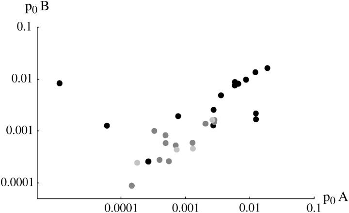
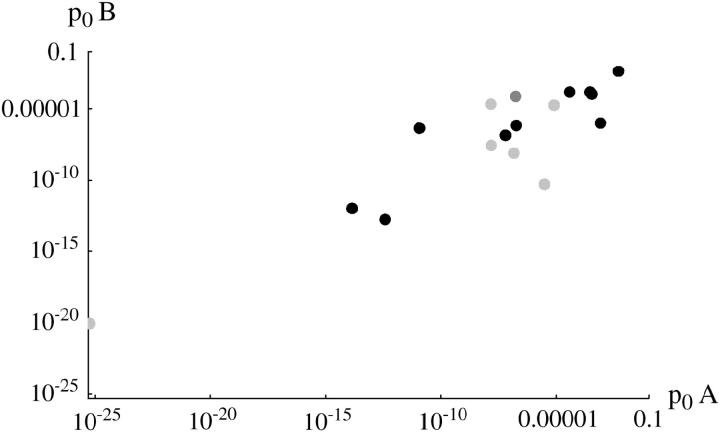
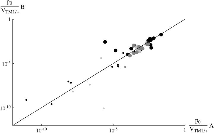
Figure 5 compares the estimated initial frequency, p₀, between replicates. The agreement between replicates indicates significant variation in p₀ among + chromosomes. For the invader lines (Figure 5, top), Kendall's rank correlation between replicates is 0.45 (P = 0.5%) for +/+ lethal and 0.53 (P = 1.0%) for the lines of Fowler et al. (1997). There is one outlier at top left (chromosome 15), in which initial frequency is much higher in replicate B compared with A. This pattern can be seen from the time course plotted in supplementary information (http://www.genetics.org/supplemental/).

Figure 5.—

Estimated initial frequencies, p₀, compared between replicates A and B. Top, “invader” lines, estimates made assuming constant fitnesses. Bottom, “transient” lines, estimates made assuming changing fitness. Solid circles, +/+ lethal; dark-shaded circles, +/+ lethal (Fowler et al. 1997); light-shaded circles, +/+ viable.

Varying fitnesses:

A model of constant fitness cannot account for those lines in which TM2 appeared at low frequency, but was later eliminated. In these cases, the fitnesses of TM2-bearing genotypes relative to TM1/+ and +/+ must have declined during the experiment, so that invasion by TM2 was possible at first, but later became impossible. We must therefore fit a model that allows for this kind of fitness variation. Unfortunately, we have much less information from which to make estimates, since TM2 never becomes common. There are several kinds of confounding evidence, which we discuss below.

We assume that the fitness of TM1/+ relative to TM2/+ increases exponentially, at a rate β per day; this allows TM2 to invade at first, but then be eliminated asTM1/+ becomes more fit. We must next choose how the other two genotypes change in fitness. In all of the lines where +/+ is viable, the relative frequencies of +/+ and TM1/+ remain constant, and so we set the fitness of both these genotypes to increase at the same rate, β. In the transient lines, TM2 remains rare, and so TM2/+ and TM1/TM2 are equally frequent in zygotes. Thus, their rate of increase depends only on the sum of their fitnesses: we have no information as to whether these fitnesses vary relative to each other. We assume that the relative fitnesses of these genotypes remain constant. Alternative assumptions would not lead to appreciably different conclusions for the transient lines, since all that can be estimated is the combined fitness of the two rare genotypes. To summarize, we introduce a single additional parameter, β, which describes the rate of increase in fitness of TM1/+ and +/+ relative to TM2/+ and TM1/TM2.

We have fitted this model of changing fitnesses to the lines in which TM2 invaded and displaced TM1, discussed above. In most cases, allowing changing fitnesses gives a significantly better fit (see rightmost columns of Table S1). Nevertheless, we give the estimates on the basis of constant fitnesses in Table S1 and used those estimates in Figures 2–5. This is because estimates made assuming varying fitness can lead to a confounding of variables, even when TM2 invades successfully, and the fitness estimates are harder to interpret when they change throughout the experiment. In any case, the patterns obtained using the alternative estimates are quite similar.

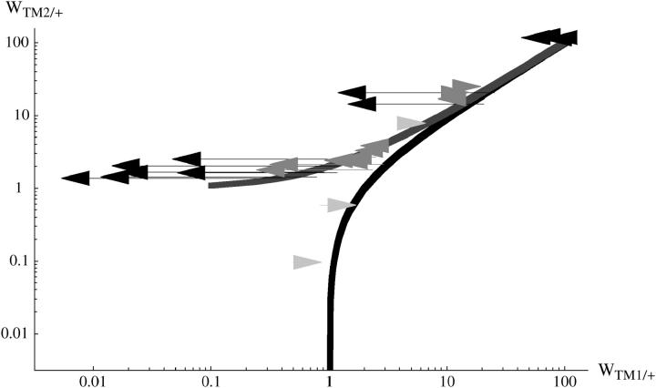
The ratio between TM1/+ fitness at the beginning of the experiment and at the end (∼300 days; e^300β) is shown under “fitness change” in Table S1. For the +/+ lethal lines, TM1/+ fitness is never estimated to increase and in most cases is estimated to decrease—often substantially. The same pattern is seen in data from Fowler et al. (1997). (This is not surprising, since a large increase in TM1/+ fitness would cause TM2 to be eliminated, as in the transient lines.) In contrast, where +/+ is viable TM1/+ is estimated to increase somewhat relative to TM1/TM2. These patterns are shown in Figure 6, in which the arrows link fitness estimates at the beginning and end of the experiment. The same patterns are seen as before (Figure 2), with clear differences between the three classes of chromosome.

Figure 6.—

Changes in fitness estimated for the invader lines. Each arrow shows estimates for a particular chromosome line, averaged over the two replicates. The base of the arrow gives fitness estimates at the beginning and the tip fitnesses at the end. Solid arrows, +/+ lethal (this experiment); dark-shaded arrows, from Fowler et al. (1997); light-shaded arrows, +/+ viable.

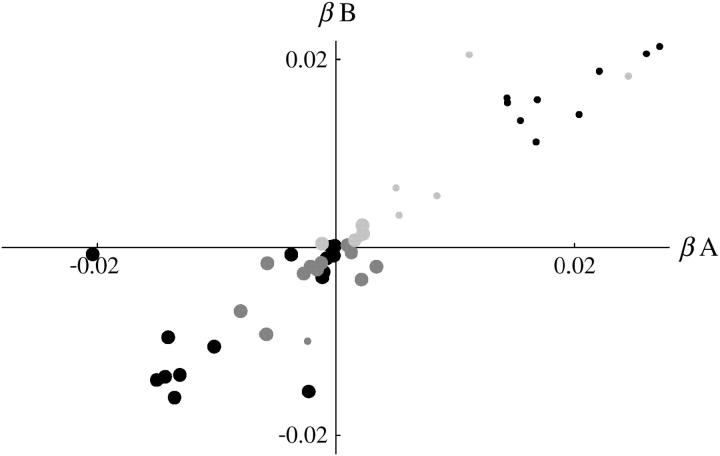
Figure 7 shows estimates of the rate of change of fitness (β per day) for all classes of chromosome. There is good agreement between replicates: for the invader lines (Figure 7, large circles), Kendall's rank correlation between replicates is 0.47 (P = 0.7%) for +/+ lethal and 0.35 (P = 8.7%) for the lines of Fowler et al. (1997). For the transient +/+ lethal lines, the correlation is 0.38 (P = 7.4%), and for +/+ viable, it is 0.60 (P = 9.5%). Taking the data as a whole, the agreement is much stronger: the circles in Figure 7 lie close to the diagonal, reflecting the similar patterns of fitness change in each replicate. Necessarily, the transient lines show an increase in TM1/+ fitness (β > 0; small circles), and the invader lines a decrease (large circles), since those lines are defined by displacement of TM1 by TM2.

Figure 7.—

Estimated rate of increase of TM1/+ fitness per day, relative to TM1/TM2, β, compared between replicates A and B. Large circles, “invader” lines; small circles, “transient” lines; solid circles, +/+ lethal; dark-shaded circles, +/+ lethal (Fowler et al. 1997); light-shaded circles, +/+ viable.

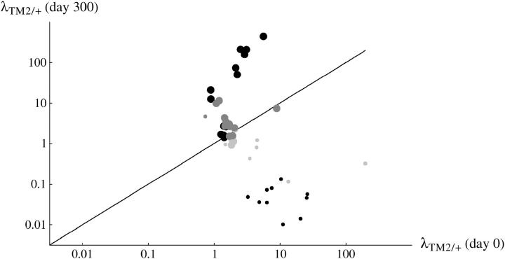
In the transient lines, TM2 never becomes common, and so only a limited set of parameter combinations can be estimated unambiguously. Table 2 summarizes these estimates and gives them in the same form for the invader lines for comparison. The rate of invasion of TM2 at the beginning and end of the experiment (λ_TM2, λ_TM2e^300β) can be estimated for all lines, and is summarized in Figure 8; the estimates here are made assuming changing fitnesses for both invader and transient lines. Overall, rates of invasion at the beginning vary much less than rates of invasion at the end—the opposite pattern to that seen for the +/+ lethal invader lines, noted above. Necessarily, rates of invasion fall from >1 to <1 in the transient lines (small circles below diagonal), whereas they rise in the invader lines (large circles above diagonal). As we saw for the fitness estimates, the lines with +/+ viable show less variation in invasion rates (light-shaded circles), as do the lines from Fowler et al. (1997)(dark-shaded circles).

Figure 8.—

The estimated rate of increase of TM2 per generation, estimated at the beginning of the experiment (horizontal) and the end (vertical). Each point is the mean across the two replicates. Large circles, “invader” lines; small circles, “transient” lines; solid circles, +/+ lethal; dark-shaded circles, +/+ lethal from Fowler et al. (1997); light-shaded circles, +/+ viable.

For the 10 chromosomes with viable +/+ homozygotes, we can estimate the frequency of +/+ adults emerging from sample vials at the beginning, when there is a stable polymorphism between +/+ and TM1/+. As noted above, this frequency stays constant throughout in the transient lines, implying constant relative fitnesses. This estimate of adult frequency is a combination of relative viability and relative fitness, which cannot be disentangled [p_+/+ = (W_TM1/+V_TM1/+)/(W_TM1/+V_+/+ + 2V_TM1/+ (W_TM1/+ − W_+/+)); Barton and Partridge 2000]. However, because the estimated fitness of +/+ is so low (at least, for the invasion lines for which it can be estimated), these frequencies reflect almost entirely the relative viability. (If TM1/+ is the only genotype that effectively reproduces, then +/+ will be at a frequency of ¹/₃ in zygotes, and variations from this in adults are due to differences in viability.) Figure S2 (supplementary information at http://www.genetics.org/supplemental/) shows the close agreement of estimates of +/+ frequency between replicates. There is a strong rank correlation between replicates, which is significant for the transient lines (0.67 among invader lines, P = 26%; 0.73 among transient, P = 4.8%). Lines that allowed successful invasion of TM2 tend to have higher +/+ viability than those in which TM2 was eliminated.

The last parameter combination that can be estimated for the transient lines is the ratio between the initial allele frequency and the viability of TM1/+ relative to TM1/TM2, p₀/V_TM1/+. These two parameters are confounded because the same observed frequencies can be generated by a high initial frequency of TM2, counterbalanced by a low viability of TM2-carrying genotypes relative to TM1/+. Figure 9 shows that again these values are similar between replicates and span a wide range of values. The estimates for the transient lines are extremely low, because the model supposes an exponential increase in fitness of TM1/+ from the beginning of the experiment. To account for a late and brief appearance of TM2, therefore, one has to assume an extremely low initial frequency and a rapid decrease in its selective advantage. In reality, the initial frequency cannot be lower than (say) 10⁻⁴, since otherwise TM2 would almost certainly be lost. Presumably the pattern of fitness change is nonlinear, so that TM2 is initially more or less neutral, then gains an advantage, and then becomes disadvantageous and is eliminated. The parameter p₀ should be thought of as indicating the delay until appearance of TM2, rather than the actual frequency.

Figure 9.—

Estimated initial frequency, relative to TM1/+ viability, compared between replicates: p₀/V_TM1/+. Large circles, “invader” lines; small circles, “transient” lines; solid circles, +/+ lethal; dark-shaded circles, +/+ lethal from Fowler et al. (1997); light-shaded circles, +/+ viable. One estimate from transient +/+ viable lines lies off scale at bottom left (chromosome 32: A, 3.7 × 10⁻²⁴; B, 1.1 × 10⁻²⁰).

Residual variation:

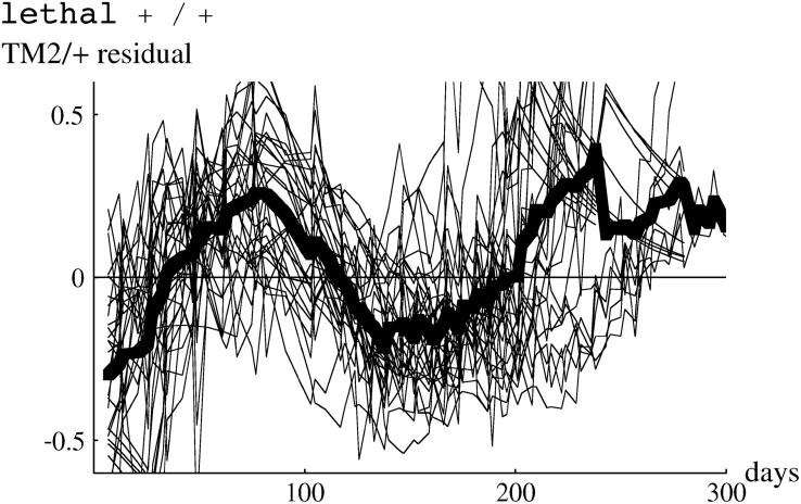
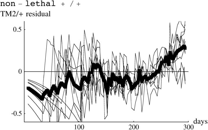
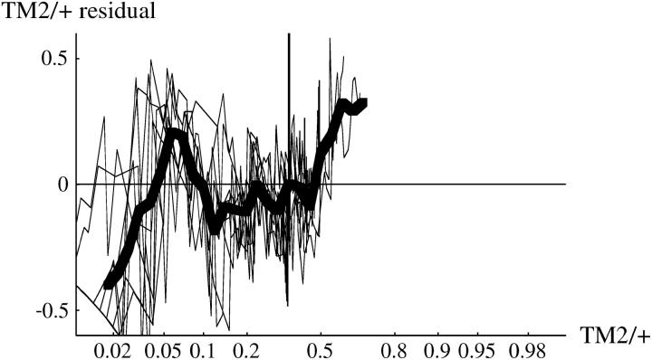
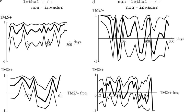
We now analyze deviations from the fitted model, as summarized in Table S1. To expand fluctuations at the extremes, we examine arcsine-transformed genotype frequencies, so that sampling variance is constant across the range of frequencies. Figure 10 (top) shows deviations of arcsine-transformed TM2/+ frequencies, for all cages in which TM2 invaded. There are clearly consistent deviations. In the lethal +/+ lines (top left), there is an excess of TM2/+ over days 30–100, then a deficit, and finally an excess beyond day 200. In the nonlethal +/+ lines (top right), there is a steady increase from a deficit of TM2/+ at first to an excess by the end. These deviations are of similar magnitude to those observed by Fowler et al. (1997)(Figure 3a). As can be seen from the examples in Figure 1, the deviations are not large: at intermediate allele frequencies (p = 0.5) the maximum mean deviation on the transformed scale corresponds to differences in allele frequency of ∼8%. Deviations of similar magnitude are seen for TM1/+. For the noninvader lines, and for +/+ frequencies, the model fits well: residual deviations are small throughout and show no consistent pattern.

Figure 10.—

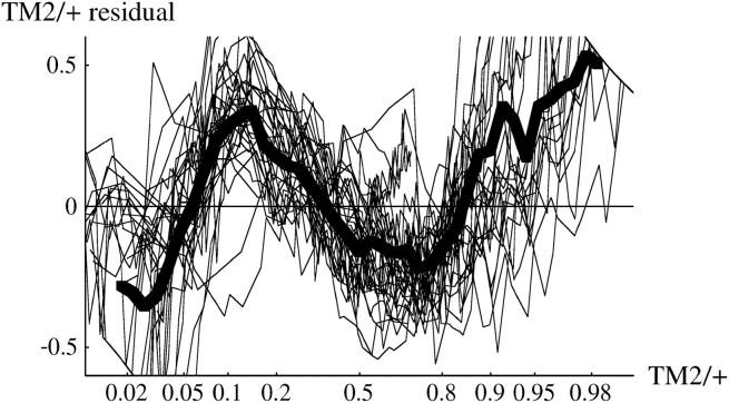
Residual deviations of TM2/+ genotype frequency from the fitted model. The left column shows the 15 lethal invader lines, and the right column shows the 4 nonlethal invader lines. The thin lines show residuals for each cage, and the thick line shows the overall average. The top row shows the residuals plotted against time, while the bottom row shows residuals plotted against predicted TM2/+ frequency, on a logit scale.

These deviations might be caused by fluctuations in relative fitness that occur at the same time, whatever the current genotype frequencies. Alternatively, there might be deviations from the model (for example, due to age structure or nonrandom mating) such that the pattern of genotype frequency change shows systematic deviations. These possibilities could be distinguished by plotting residuals against predicted genotype frequency, rather than against time. Fowler et al. (1997)(Figure 3b) found that overall residual deviations were smaller when plotted against genotype frequency rather than against time, suggesting that the deviations are due to environmental factors that occur on particular days rather than factors acting at particular stages of the invasion. In our experiment, deviations show a similar pattern when plotted against frequency rather than time (Figure 10, bottom), so that we cannot distinguish between the alternative explanations. The similarity of the two kinds of plots is not due to the invasions occurring at similar times in our experiment: the variance of log(p₀) is somewhat higher for our invader lines than for Fowler et al.'s (1997) experiment.

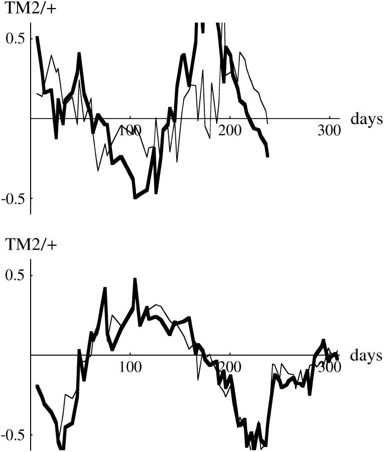
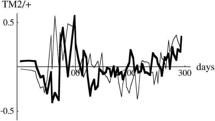
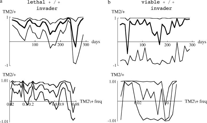
Figure 11 shows some examples of how deviations change through time for three pairs of replicate cages (Figure 1, chromosomes 3, 30, and 34). The overall mean across all cages in each class (i.e., Figure 10, top row, thick lines) has been subtracted, so that these plots show the deviations peculiar to each cage. There is extraordinary consistency between replicate cages, which is even more marked than that seen by Fowler et al. (1997)(Figure 4). Figure 12 shows the correlation between replicates, within a moving window. These plots are analogous to Fowler et al.'s (1997) Figure 5 and show much stronger correlations throughout. As in Figure 10, similar patterns are seen whether plots are against time (top row) or against frequency (bottom row). Strong correlations are seen for noninvader lines as well as invaders, even though the deviations are smaller in this case. Confidence intervals are wide for any one window (Figure 12, thin lines), especially where only a few chromosome lines are in each class (for example, only four nonlethal +/+ lines invaded; Figure 12b). It is not clear how to make an overall test for significance, since successive deviations are autocorrelated. However, individual correlations are significant in most cases for the lethal +/+ lines (Figure 12, a and c), and the overall pattern is compelling. Indeed, correlations between replicates are about as high as they could be, given sampling error. For each pair of replicate cages, we can calculate the difference in arcsine-transformed genotype frequency, for those cases where sampling dates coincide. This difference has sampling variance 4/N_A + 4/N_B. For each replicate pair, we calculated the ratio between the variance of between-replicate differences and that expected from sampling error. Averaging over pairs, the ratio averages 1.27 for lethal +/+ invader lines and 1.58 for viable +/+ invader lines. Thus, most of the variance between replicates is due to sampling error.

Figure 11.—

Examples of residual deviations from the fitted model, for the three chromosomes shown in Figure 1 (left). (Top to bottom, chromosomes 3, 30, and 34). Each graph shows the deviation in arcsine-transformed frequency of TM2/+, for the two replicate cages (thin and thick lines). The overall mean deviation (Figure 10, top row, thick line) has been subtracted, so that these plots show the deviations peculiar to each chromosome line.

Figure 12.—

Correlations of residual deviations between replicates. The thick line shows the correlation within a moving window, while the thin lines show 95% confidence intervals (using Fisher's tanh approximation). Correlations are plotted against time for the top of a–d and against frequency for the bottom of a–d, as in Figure 10.

DISCUSSION

The key finding of our study is that there are large and highly replicable fitness differences between genotypes carrying different wild-type chromosomes. Strikingly, all 40 replicate pairs of cages showed the same class of pattern: in every case, if TM2 replaced TM1 in one cage, it also did so in the partner cage; if TM2 failed to invade in one cage, it also failed in the partner cage. Over shorter timescales, fluctuations were correlated between replicate cages. These transient patterns imply that relative fitnesses are changing through the experiment. Thus, the pattern of genetic variation cannot be summarized in one simple measure, such as the additive variance in fitness.

The 15 chromosomes for which +/+ was lethal and where TM2 invaded successfully showed a similar pattern of invasion to the lines in Fowler et al. (1997). Moreover, the effects on TM1/+ and on TM2/+ are strongly correlated, indicating that variation is largely additive (Figure 2). However, the rate of invasion of TM2 varies greatly between chromosomes, but the rate of elimination of TM1 is more similar between chromosome lines and on average slower. Hence there is significantly greater fitness variance between TM1/+ than between TM2/+: variance in log_e (fitness) is 1.62 for TM1/+, compared with 0.46 for TM2/+. This indicates that although the effects of + chromosomes on the fitness of the two different heterozygous genotypes are strongly correlated, the magnitude of the effect is greater in the less fit genotype. This can be seen as an example of synergistic epistasis, in which deleterious alleles tend to magnify each other's effects (Peters and Keightley 2000). Our method could be extended to measure the magnitude of such epistasis, by observing the total fitness of recombinant chromosomes (Fowler et al. 1997; Barton and Partridge 2000).

We should emphasize that we have measured only the effects of whole chromosomes on fitness and so can say nothing about within-chromosome epistasis: the strong fitness effects that we observe are the aggregate effect of (presumably) large numbers of loci on the third chromosome. Thus, our comments on additive vs. dominance effects refer only to whole nonrecombining chromosomes, treated as single genetic loci. However, we can investigate genetic correlations between fitness components, and our technique could be applied to measure the effects of recombinant chromosomes on fitness. The extraordinary replicability and large magnitude of the fitness variation suggest that this would be a powerful way of investigating epistasis and recombination.

For the four lines in which TM2 invaded, and +/+ was viable, we could estimate the fitness of +/+ homozygotes, relative to the double-balancer genotype, TM1/TM2; these estimates were extremely low. In several studies (e.g., Sved 1971, 1975), the fitness of wild-type homozygotes has been measured relative to the heterozygote with the balancer. In these studies, the mean fitness of +/+ homozygotes relative to the heterozygotes was 0.34 ± 0.05 (Sved 1971) and 0.23 ± 0.06 (Sved 1975). However, in 7 out of 34 of Sved's chromosome lines, the relative fitness of +/+ homozygotes was found to be zero. Thus, although both Sved's and our experiments found low homozygous fitness, our estimates are significantly lower. One possibility is that our cages provide harsher environments than was the case in earlier experiments: wild-type homozygotes may be unable to reproduce in crowded cages, even if they can survive to adulthood under benign conditions. Indeed, the range of size variation among flies in cages is much greater than that normally found in bottle cultures and such morphological differences might be correlated with fertility. In this and earlier studies, mean homozygous fitnesses are much lower than mean homozygous viabilities, each being measured relative to heterozygotes (arithmetic mean fitness vs. viability is 0.015 vs. 1.16 here, compared with 0.34 vs. 0.73 in Sved 1971 and 0.23 vs. 0.75 in Sved 1975). Thus, the effect of homozygosity on fitness is much more severe than its effects on viability.

A puzzling result is that viabilities measured in controlled crosses (Gardner et al. 2001) and measured among offspring of females sampled from the cages are weakly correlated, even though larvae were reared in vials in a similar way in each case. (There is a significant correlation between experiments when data are averaged over TM1/+ and TM2/+ and over replicates, but not otherwise; Figure 4.) In contrast, Sved (1971)(1975) found a strong correlation between frequencies of adults in ratio tests and in cages (r = 0.77, d.f. = 22, P < 0.001; r = 0.86, d.f. = 12, P < 0.001 respectively). Our estimates of viability based on females sampled from the cages do depend on the assumption that when TM2 is rare, the two rare genotypes TM2/+ and TM1/TM2 each mate with the common TM1/+ genotype, so that they are at the same frequency in zygotes. This assumption could be violated if flies bearing the rarer balancers were to seek out and mate with other rare genotypes; however, this seems extremely implausible. The rather weak correlation between independent measures of viabilities remains puzzling to us, especially since overall fitness measures are so highly replicable.

Perhaps the most striking feature of our results is that relative fitnesses change substantially through time. This is shown both by the overall pattern and by shorter-term fluctuations in genotype—both strongly correlated across replicates. In 14 of the 40 lines, TM2 appeared at low frequency, but later disappeared. This implies that TM2 was initially more or less neutral, so that it persisted at low frequency for several months and then gained an advantage and rose to appreciable frequency and finally lost this advantage and was eliminated from the cage. Even after allowing for a long-term decline in fitness of TM2 relative to TM1, there were significant residual fluctuations, peculiar to each wild-type chromosome (Figures 10–12). These changes in relative fitness over time could be due to subtle changes in external environment common to all cages (for example, slight differences in food quality); to intrinsic changes in the cages (for example, due to a changing age structure); or to changes in genotype frequency, which alter the environment experienced by each individual. Direct frequency dependence seems unlikely, because fitnesses would have to change substantially as a function of the frequency of extremely rare genotypes: in particular, it is hard to see how, in the transient lines, TM2 could begin increasing after a long period at undetectably low frequency, but then decline before reaching 10% of the population (see Figure 1, right).

Whatever the cause of a changing environment, there must be strong genotype × environment interactions: different wild-type chromosomes show different patterns through time (Figure 11). There is evidence from other Drosophila experiments for genotype × environment interaction for total fitness (Mackay 1986; Fowler et al. 1997; and for components of fitness Mackay 1986; Wayne et al. 1997). While there is evidence that viability of Drosophila larvae is frequency dependent (Curtsinger 1990; Curtsinger and Sheen 1991), there is little evidence concerning frequency dependence of net fitness (although see Curtsinger 1990).

The results in this article, together with the study by Fowler et al. (1997), show that fitness differences are extremely strong and highly heritable. This contrasts with other studies on viability variation in Drosophila (Charlesworth 1987). For example, Mukai and Nagano (1983) estimated the variance in log_e (heterozygous viability) to be 0.023, which compares with 0.165 in Gardner et al. (2001) and 0.208 in this study (averaged across TM1/+ and TM2/+, correcting for between-replicate variance, and including only invasion lines for which both relative viabilities could be estimated; Table S1). One possibility is that the effects of wild-type chromosomes are greater when they are held against unfit balancer chromosomes (see below). However, the earlier experiments also used balancers, and so this explanation is not compelling. Our experiment differs from earlier ones in that heterozygote fitnesses are measured relative to a standard genotype, TM1/TM2, rather than against +/+. The low viability of the double balancer will introduce extra sampling error into estimates of relative viability, but since results are highly replicable, this does not account for the high genetic variance in heterozygous viability that we have observed.

In our experiment, we have found strong and replicable fitness differences, which change substantially through time. What does this tell us about the genetic basis of fitness variation in general? An obvious issue is whether cage populations of Drosophila are representative of natural populations. Although we were careful to carry out the experiment under the conditions to which the Dahomey population had adapted, over 30 years in the laboratory, the changes in fitness that we observed presumably reflect changes in environment that were beyond our control. However, natural environments also change: we believe that it is reasonable to take our experimental populations as more or less typical of local populations in nature. A more serious concern is that wild-type chromosomes were held against balancers, which are lethal as homozygotes and cause substantially reduced fitness when heterozygous. Loss of function of the balancers may reveal variation between wild-type chromosomes, both because recessive alleles are unmasked when combined with deleterious alleles at homologous loci and because of synergistic epistasis. The ideal would be to use freshly constructed balancers, marked by molecular variants rather than by dominant phenotypic mutations.

Our results suggest that populations contain abundant fitness variation, which can sustain adaptive selection and shape the genetic system (i.e., recombination rates, life history, mate preferences, and so on). However, a single measure, such as the additive genetic variance in fitness, cannot adequately represent the substantial variations through time that we observed: we have avoided calculating such a measure, because it would depend on arbitrary assumptions about when during the experiment to calculate fitness and how additive effects at individual loci relate to net chromosomal fitness. The high variability we see is incompatible with the “classical” view, in which genetic variation is maintained by an equilibrium between deleterious mutations and selection (Lewontin 1974). It is possible that fluctuating selection itself maintains variation. With selection alone, this requires effective overdominance (Haldane and Jayakar 1963); if there is a low rate of mutation, other mechanisms can be effective (e.g., Kondrashov and Yampolsky 1996; Burger 1999, Waxman and Peck 1999; Turelli and Barton 2004). However, such mechanisms are difficult to reconcile with the observed slow rates of molecular evolution (Kimura 1983): fluctuating selection at individual loci would be expected to cause frequent amino acid substitution. This makes it plausible that balancing selection maintains strongly selected polymorphisms at many loci, but that the fitnesses of the genotypes involved are sensitive to environmental conditions, leading to the strong fluctuations in net fitness that we have observed. The remarkable replicability of these fluctuations suggest many possibilities for further investigation.

References

- Barton, N. H., and L. Partridge, 2000. Measuring fitness by means of balancer chromosomes. Genet. Res. 75: 297–314. [DOI] [PubMed] [Google Scholar]
- Burger, R., 1999. Evolution of genetic variability and the advantage of sex and recombination in changing environments. Genetics 153: 1055–1069. [DOI] [PMC free article] [PubMed] [Google Scholar]
- Burt, A., 1995. The evolution of fitness. Evolution 49: 1–8. [DOI] [PubMed] [Google Scholar]
- Charlesworth, B., 1987 The heritability of fitness, pp. 21–40 in Sexual Selection: Testing the Alternatives, edited by J. W. Bradbury and M. B. Anderson. John Wiley & Sons, New York.
- Clutton-Brock, T. H. (Editor), 1988 Reproductive success: studies of individual variation in contrasting breeding systems, pp. 472–485 in Reproductive Success. University of Chicago Press, Chicago.
- Curtsinger, J. W., 1990. Frequency-dependent selection in Drosophila: estimation of net fitness in pseudohaploid populations. Evolution 44: 857–869. [DOI] [PubMed] [Google Scholar]
- Curtsinger, J. W., and R. Ming, 1997. Non-linear selection response in Drosophila: a strategy for testing the rare-alleles model of quantitative genetic variability. Genetica 99: 59–66. [DOI] [PubMed] [Google Scholar]
- Curtsinger, J. W., and F. M. Sheen, 1991. Frequency-dependent viability in mutant strains of Drosophila melanogaster. J. Hered. 82: 105–109. [DOI] [PubMed] [Google Scholar]
- Fisher, R. A., 1930 The Genetical Theory of Natural Selection. Oxford University Press, Oxford.
- Fowler, K., C. Semple, N. H. Barton and L. Partridge, 1997. Genetic variation for total fitness in Drosophila melanogaster. Proc. R. Soc. Lond. Ser. B 264: 191–199. [DOI] [PMC free article] [PubMed] [Google Scholar]
- Gardner, M., K. Fowler, L. Partridge and N. H. Barton, 2001. Genetic variation for preadult viability in Drosophila melanogaster. Evolution 55: 1609–1620. [DOI] [PubMed] [Google Scholar]
- Gibson, J. R., A. K. Chippindale and W. R. Rice, 2002. The X chromosome is a hot spot for sexually antagonistic fitness variation. Proc. R. Soc. Lond. Ser. B 269: 499–505. [DOI] [PMC free article] [PubMed] [Google Scholar]
- Gillespie, J. H., 2001. Is the population size of a species relevant to its evolution? Evolution 55: 2161–2169. [DOI] [PubMed] [Google Scholar]
- Haldane, J. B. S., and S. D. Jayakar, 1963. Polymorphism due to selection of varying direction. J. Genet. 58: 237–242. [Google Scholar]
- Kimura, M., 1983 The Neutral Theory of Molecular Evolution. Cambridge University Press, Cambridge, UK.
- Kondrashov, A. S., and D. Houle, 1994. Genotype-environment interactions and the estimation of the genomic mutation-rate in Drosophila melanogaster. Proc. R. Soc. Lond. Ser. B 258: 221–227. [DOI] [PubMed] [Google Scholar]
- Kondrashov, A. S., and L. Y. Yampolsky, 1996. High genetic variability under the balance between symmetric mutation and fluctuating stabilizing selection. Genet. Res. 68: 157–164. [Google Scholar]
- Kruuk, L. E. B., T. H. Clutton Brock, J. Slate, J. Pemberton, S. Brotherstone et al., 2000. Heritability of fitness in a wild mammal population. Proc. Natl. Acad. Sci. USA 97: 698–703. [DOI] [PMC free article] [PubMed] [Google Scholar]
- Lenski, R. E., and M. Travisano, 1994. Dynamics of adaptation and diversification: a 10,000 generation selection experiment with bacterial populations. Proc. Natl. Acad. Sci. USA 91: 6608–6618. [DOI] [PMC free article] [PubMed] [Google Scholar]
- Lewontin, R. C., 1974 The Genetic Basis of Evolutionary Change. Columbia University Press, New York.
- Mackay, T. F. C., 1986. A quantitative genetic analysis of fitness and its components in Drosophila melanogaster. Genet. Res. 47: 59–70. [Google Scholar]
- Merila, J., and B. Sheldon, 2000. Lifetime reproductive success and heritability in nature. Am. Nat. 155: 301–310. [DOI] [PubMed] [Google Scholar]
- Mukai, T., and S. Nagano, 1983. The genetic structure of natural populations of Drosophila melanogaster. XVI. Excess of additive genetic variance of viability. Genetics 105: 115–134. [DOI] [PMC free article] [PubMed] [Google Scholar]
- Mukai, T., and O. Yamaguchi, 1974. The genetic structure of natural populations of Drosophila melanogaster. XI. Genetic variability in a local population. Genetics 76: 339–366. [DOI] [PMC free article] [PubMed] [Google Scholar]
- Partridge, L., and K. Fowler, 1992. Direct and correlated responses to selection on age at reproduction in Drosophila melanogaster. Evolution 46: 76–91. [DOI] [PubMed] [Google Scholar]
- Partridge, L., and K. Fowler, 1993. Responses and correlated responses to artificial selection on thorax length in Drosophila melanogaster. Evolution 47: 213–226. [DOI] [PubMed] [Google Scholar]
- Peters, A. D., and P. D. Keightley, 2000. A test for epistasis among induced mutations in Caenorhabditis elegans. Genetics 156: 1635–1647. [DOI] [PMC free article] [PubMed] [Google Scholar]
- Simmons, M. J., and J. F. Crow, 1977. Mutations affecting fitness in Drosophila populations. Annu. Rev. Genet. 11: 49–78. [DOI] [PubMed] [Google Scholar]
- Stearns, S. C., 1992 The Evolution of Life Histories. Oxford University Press, Oxford.
- Sved, J. A., 1971. An estimate of heterosis in Drosophila melanogaster. Genet. Res. 18: 97–105. [DOI] [PubMed] [Google Scholar]
- Sved, J. A., 1975. Fitness of third chromosome homozygotes in Drosophila melanogaster. Genet. Res. 25: 197–200. [DOI] [PubMed] [Google Scholar]
- Teotónio, H., M. Matos and M. R. Rose, 2002. Reverse evolution of fitness in Drosophila melanogaster. J. Evol. Biol. 15: 608–617. [Google Scholar]
- Turelli, M., and N. H. Barton, 2004. Polygenic variation maintained by balancing selection: pleiotropy, sex-dependent allelic effects and G × E interactions. Genetics 166: 1053–1079. [DOI] [PMC free article] [PubMed] [Google Scholar]
- Waxman, D., and J. R. Peck, 1999. Sex and adaptation in a changing environment. Genetics 153: 1041–1053. [DOI] [PMC free article] [PubMed] [Google Scholar]
- Wayne, M. L., J. B. Hackett and T. F. C. Mackay, 1997. Quantitative genetics of ovariole number in Drosophila melanogaster. I. Segregating variation and fitness. Evolution 51: 1156–1163. [DOI] [PubMed] [Google Scholar]
- Weber, K. E., 1996. Large genetic change at small fitness cost in large populations of Drosophila melanogaster selected for wind tunnel flight: rethinking fitness surfaces. Genetics 144: 205–213. [DOI] [PMC free article] [PubMed] [Google Scholar]