Combining Data From Multiple Inbred Line Crosses Improves the Power and Resolution of Quantitative Trait Loci Mapping

Abstract

Rodent inbred line crosses are widely used to map genetic loci associated with complex traits. This approach has proven to be powerful for detecting quantitative trait loci (QTL); however, the resolution of QTL locations, typically ∼20 cM, means that hundreds of genes are implicated as potential candidates. We describe analytical methods based on linear models to combine information available in two or more inbred line crosses. Our strategy is motivated by the hypothesis that common inbred strains of the laboratory mouse are derived from a limited ancestral gene pool and thus QTL detected in multiple crosses are likely to represent shared ancestral polymorphisms. We demonstrate that the combined-cross analysis can improve the power to detect weak QTL, can narrow support intervals for QTL regions, and can be used to separate multiple QTL that colocalize by chance. Moreover, combined-cross analysis can establish the allelic states of a QTL among a set of parental lines, thus providing critical information for narrowing QTL regions by haplotype analysis.

QUANTITATIVE trait locus (QTL) analysis is a phenotype-driven, experimental approach to identify genomic regions that harbor polymorphisms affecting the distribution of a measurable trait in a mapping population. Knowledge of the number, location, and effects of the genetic loci underlying variability in a trait can aid our understanding of the biochemical basis of the trait. Despite the power of QTL analysis, the mapping approach has some limitations. Detection of a QTL with desirable power and accuracy in an inbred line cross depends on the genetic diversity between the parental strains, heritability of the trait, the size of the cross, and the density of genetic markers (Kao and Zeng 1997). In a single intercross or backcross, it may be difficult to distinguish multiple tightly linked QTL from a single QTL of large effect. Furthermore, the QTL support interval may be large, typically 20–40 cM for mouse crosses. Investigators often encounter difficulty when they attempt to narrow the QTL region. Adding markers is helpful but resolution is fundamentally limited by the number of recombination events in the cross population. The direct approach to narrowing a QTL region is to pursue mapped loci as targets for positional cloning by isolating the QTL region on a fixed background in a congenic strain, using additional crosses to fine map, and then applying techniques such as BAC rescue to identify the gene (Glazier et al. 2002; Abiola et al. 2003). This seemingly straightforward strategy has proven to be challenging in many cases (Nadeau and Frankel 2000), although more optimistic views on the situation have also been expressed (Korstanje and Paigen 2002).

Many common diseases in humans including osteoporosis, atherosclerosis, diabetes, and hypertension are known to be complex—determined by the interaction of multiple genetic and environmental factors. Rodent inbred lines can model human disease traits and inbred line crosses provide a powerful approach to mapping the genetic loci associated with these diseases (Paigen 1995). In many instances, disease-related traits have been studied in multiple mouse crosses. We propose a strategy to improve the power and resolution of QTL mapping by utilizing the combined information in two or more inbred line crosses. These crosses may or may not include parental lines in common. In any single cross of two strains, we are limited to discovering only loci that show allelic variation between those strains. By looking at multiple crosses, we can sample more allelic variation, and thus we have an opportunity to detect additional loci that can be implicated in a disease model. If QTL appearing in multiple crosses represent the same ancestral polymorphic loci, then by combining crosses we can achieve greater sample size and power for detecting and localizing these shared QTL.

Statistical methods for QTL analyses of mapping populations derived by crossing two inbred parental strains are well developed (Lander and Botstein 1989; Haley and Knott 1992; Jansen and Stam 1994; Zeng 1994; Sen and Churchill 2001). Multiple-strain crosses and the combination of multiple crosses each from two inbred parental strains have been explored as methods for QTL detection using multiple-allele models (Zeng 1994; Liu and Zeng 2000). Several reports describing combined QTL analysis have appeared recently (Walling et al. 2000; Hitzemann et al. 2003; Park et al. 2003) and we expect this trend to continue. When a cross involves two inbred strains, only two alleles are segregating at any given locus. However, in outbred crosses or multiway crosses, it is usual to assume that multiple alleles are segregating at any given locus. The statistical models required represent a straightforward extension of the usual two-allele models. For example, Rebai et al. (1994) adapted the regression method (Haley and Knott 1992) to the case of intercross populations derived from a diallele of multiple inbred lines. However, multiple-allele modeling of the background genetic variance in this setting may become formidably complex and can impact the overall power to detect QTL. Ignoring background genetic variation may lead to biases in estimates of QTL location and effects (Zou et al. 2001). An interesting proposal to map QTL by genetic background interactions in a set of three intercrosses involving three parental strains was put forth by Jannink and Jansen (2001)(Jansen and Stam 1994). Multiple-allele models are general because they can accommodate any pattern of inheritance but this generality can result in a loss of power to detect QTL.

Inbred laboratory mouse strains are known to have originated from a mixed but limited founder population (Silver 1995; Beck et al. 2000). The genomes of these strains were predicted to be a mosaic of regions with origins that can be traced back to a few subspecies (Bonhomme 1986). The mosaic structure of variation in the laboratory mouse genome was recently evidenced by single-nucleotide polymorphism (SNP) analyses indicating that inbred laboratory mouse strains are largely derived from two original subspecies (Mus mus domesticus and M. m. musculus) with limited contributions from M. m. castaneus. Indeed, for most of the regions investigated, only two different ancestral haplotypes were observed among nine strains (Wade et al. 2002). This observation suggests that we may be able to improve the power and resolution of QTL detection by combining data from two or more inbred line crosses that involve multiple strains by assuming a common biallelic mode of inheritance. Even in cases where the locus in question is not strictly biallelic, the effects of a shared QTL may behave as a biallelic locus having only “high” and “low” alleles.

In this article, we report a simple but effective approach for improving the power and resolution of QTL detection using combined data from two or more inbred strain crosses. We propose a binary encoding based on the biallelic hypothesis to reduce the number of alleles in the genetic model. Recoding improves power when the correct biallelic state of the QTL is identified. However, it is not possible to know a priori the allelic states of QTL and different QTL in the same cross may have different patterns of alleles across the parental strains. The strategy proposed here can exploit the power of a biallelic model but does not lose information or restrict the possible allelic states of the QTL.

MATERIALS AND METHODS

Combined-cross analysis overview:

A combined-cross analysis involves several steps of data processing and interpretation. Details of each step are provided in the sections that follow. Here we provide an overview to tie the various steps together. It is important to emphasize that this is not a rigid prescription. Each combined data analysis will present unique challenges and the process of interpretation should be adaptive and interactive.

A preliminary step to combining crosses is to carry out an analysis of each individual cross. This will provide a sense of the number and locations of QTL, their mode of inheritance, and direction of effects. If the individual crosses are small, which may be the case if the experiment was designed with the intent to combine the data, they may have low power to detect QTL. A less stringent assessment of the presence of QTL may be appropriate at this stage. A shared QTL is one that occurs in all of the crosses. Thus the locus must be polymorphic within each pair of parental lines represented in the set of crosses. A cross-specific QTL will occur in only one or in a subset of the crosses. If a cross-specific QTL occurs in more than one but not all of the crosses, it can be analyzed as a shared QTL on the subset of crosses in which it does occur. The goals of a combined-cross analysis are to identify shared and cross-specific QTL and to improve the localization of shared QTL.

The next steps are merging the data and running a genome-wide scan analysis on the combined data. It is assumed that the phenotype data are measuring the same trait in all crosses. Some care must be taken to scale data before merging them. An indicator variable, cross, is created and included along with any other covariates that may be relevant to the analysis. The genotype data are merged using a binary encoding that reflects the expected allele types of a shared QTL. This encoding may be based on the parental phenotypes. Now we can carry out a combined-cross genome scan using cross as an additive covariate (Comb1) to detect shared QTL. Then we carry out a genome scan using cross as an interactive covariate (Comb2) to detect cross-specific QTL. A significant change in the LOD score (ΔLOD1) between these scans indicates that a QTL has cross-specific effects.

The final steps involve a local analysis of each chromosome that was identified in the combined data genome scans. We test for presence of two or more linked QTL by computing the change in likelihood between the one QTL and the two QTL scans (ΔLOD2) on each chromosome of interest. High-resolution plots of the single and pairwise scans can indicate the presence of multiple QTL even when a formal test is not significant. The local analysis is intended to clarify the nature of QTL that have already been declared to be significant in the genome-wide scans. In addition, one should consider the estimated effects of the QTL in the individual and combined crosses. A set of QTL allele-effect plots at critical locations along a chromosome can help to resolve linked and cross-specific QTL.

Experimental breeding crosses for QTL mapping:

We use data from four intercross populations involving five strains to illustrate our method. The five strains (and single-letter abbreviations used in this article) are PERA/Ei (P), I/LnJ (I), DBA/2 (D), CAST/Ei (C), and 129S1/SvImJ (S). The four crosses, three of which have been previously described, are P × I (Wittenburg et al. 2003), P × D, C × D (Lyons et al. 2003a), and C × S (Lyons et al. 2003b). Mice in each of the crosses were assayed under high-fat diet conditions (Khanuja et al. 1995) for plasma high-density lipoprotein (HDL) cholesterol. The P × I cross includes 305 mice genotyped at 107 markers; P × D has 324 mice and 97 markers; C × D has 278 mice and 109 markers; C × S has 277 mice and 100 markers. Crosses P × I and P × D include both sexes but crosses C × D and C × S include only males. In each of the crosses, F₂ progeny were obtained from F₁ parents using both directions of crossing, e.g., P × I and I × P, where the first letter denotes the strain of the maternal parent of the F₁ mice used to generate the F₂ progeny. Further details are provided in the references listed above.

Combining the phenotype data:

Plasma HDL cholesterol was measured in milligram per deciliter units as described in (Lyons et al. 2003a). Both the mean and the variance of HDL cholesterol varied significantly across the four intercross populations. Box plots of the raw and transformed data (Figure 1) indicate that a logarithmic transform overcorrects the variance heterogeneity, whereas square-root transform, an intermediate between the logarithmic and untransformed data, stabilizes the variance in HDL levels. Transformation of data is often applied to achieve approximate normality of residual effects. In a combined-cross analysis, crosses with greater variability in the phenotype will have a greater influence. Thus, it is important to stabilize the variances in this setting. If no simple transformation is able to achieve this, data could be standardized within crosses before combining. In this case, we used the square-root transform of HDL in all subsequent analyses.

Figure 1.—

Box plots of the HDL phenotype by cross. Logarithmic, square-root, and untransformed data are shown.

QTL mapping methods (single-cross analysis):

We carried out genome-wide scans for both main-effect and interacting QTL in individual crosses using the method of Sen and Churchill (2001). Logarithm of odds ratio (LOD) scores were computed at 2-cM intervals across the genome and significance was determined by permutation testing (Churchill and Doerge 1994). Following the guidelines proposed by Lander and Kruglyak (1995) we interpret the 0.05 and 0.63 levels as significant and suggestive, respectively. (Note that in the original reports of these crosses we used a more stringent definition of suggestive QTL, P < 0.10, genome-wide adjusted.) Simultaneous-search genome scans for all pairs of markers were carried out to detect epistatic interactions (Sen and Churchill 2001; Sugiyama et al. 2001). Significant QTL-by-QTL interactions are detected as locus pairs with significant (P < 0.05, genome-wide adjusted) joint LOD score and a significant (P < 0.001, unadjusted) interaction component. Support intervals for QTL localization were computed by the method of Sen and Churchill (2001).

Integration of genetic marker data:

Genetic map positions for markers in each of the crosses in this study were retrieved from the Mouse Genome Database (http://www.informatics.jax.org). When multiple crosses share the same set of markers, integration of the marker genotype data is straightforward. However, data may be merged even if different markers were used, provided that a reliable map order and approximate genetic map positions (in centimorgan units along each chromosome) are known. Genetic distances between marker loci may vary somewhat from cross to cross but the precise location of markers on the genetic map has little practical impact on QTL analysis. Correct relative ordering of markers is crucial for combining the genotype data. To merge the data sets in this study, we computed a set of 128 multiple imputed genotypes on a dense (2-cM) grid of genomic locations, using the same grid for each cross. We then merged the imputed data sets and carried out QTL analysis using the method of Sen and Churchill (2001). In principle the same analysis could be carried out using an EM algorithm (Lander and Botstein 1989; Kao and Zeng 1997), but the simplicity of merging imputed data sets is appealing in this application.

Binary encoding of alleles for combined-cross analysis:

The power of the genome-wide combined-cross analysis is achieved by recoding of the parental alleles to a binary allelic pattern. The choice of recoding schemes will depend on the particular set of crosses under consideration. In our example the crosses form a chain (I × P × D × C × S) in which the phenotypes of the parental strains are alternating. Strains P and C have high HDL cholesterol and strains I, D, and S have low HDL cholesterol levels. This suggests a binary recoding of alleles as shown in Figure 2.

Figure 2.—

Binary encoding of alleles for combined-cross analysis of HDL.

In a combined-cross analysis any two strains that are paired in an individual cross should have distinct codes (i.e., all crosses are A × B) and an indicator for the cross should be retained in the recoded data. In this way we can ensure that no information is lost. The original identity of any genotype can always be recovered by knowing which cross the animal came from and which strains are coded as A and B in that cross. Any crosses between two strains that would both be coded as A (or B) should be left out of a combined-cross analysis as they will be uninformative.

Having selected a recoding scheme for combining crosses, we must immediately acknowledge that not all QTL in the cross will share the same distribution of allelic states across the set of parental lines. Indeed, transgressive QTL for which a low parent may contribute a high allele are common. Recoding focuses our search on the most likely QTL configurations. At the same time we need to ensure that we do not miss QTL that have other allele distributions across the strains. QTL that fail to meet our expectations can still be detected and analyzed as described below. We considered the possibility of genome-wide scans using all possible binary recoding of alleles. However, this approach raises issues of multiple testing that are likely to offset any advantages of the binary QTL model.

Decoding allelic distributions from QTL peaks:

Suppose we have carried out genome scans on several individual crosses. Ideally we will know for each cross whether the QTL is present or absent. In practice, there will be a gray area and this could lead to some ambiguity in interpretation. If a QTL is present, the parental strain must carry different alleles and, if it is absent, parental strains will carry the same allele or alleles that do not differ in effect. Thus the pattern of presence or absence of QTL peaks provides information about the allelic distribution across the strains in a set of crosses. When the crosses form a chain, it is possible to uniquely determine the allelic distribution of a QTL from the pattern of presence or absence in the individual cross genome scans (see Table 1). If the chain is closed to form a loop of crosses (by adding cross I × S in this case), a confirmatory prediction is obtained. This redundant information could provide a check of the biallelic model. For other sets of crosses several allelic distributions may be consistent with the observed pattern of QTL peaks. In practice, some care is needed to properly interpret a pattern of QTL peaks in multiple crosses. Whereas significant peaks clearly indicate the presence of a QTL, the absence of a peak can be ambiguous. It is helpful to examine the “shape” of the LOD curve to detect clues that multiple linked QTL may be present. The direction of locus-specific allele effects in each cross can provide additional evidence regarding the parental distribution of QTL alleles.

TABLE 1.

Decoding binary allele patterns from QTL peaks

P × I	P × D	C × D	C × S	Pattern	Prediction I × S	QTL
+	−	−	−	PDCS:I	+	Chr 5 at 2 cM
−	+	−	−	PI:DCS	+
−	−	+	−	PID:CS	+	Chr 2 at 48 cM
−	−	−	+	PIDC:S	+
+	+	−	−	P:IDCS	−	Chr 11 at 20 cM
+	−	+	−	PD:ICS	−
+	−	−	+	PDC:IS	−
−	+	+	−	PICS:D	−
−	+	−	+	PIS:DC	−	Chr 1 at 86 cM
−	−	+	+	PIDS:C	−	Chr 6 at 68 cM
+	+	+	−	PCS:ID	+
+	+	−	+	PS:IDC	+
+	−	+	+	PDS:IC	+
−	+	+	+	PIC:DS	−
+	+	+	+	PC:IDS	−	Chr 4 at 22 cM

Column 5 lists all possible bipartitions of QTL alleles among five strains. In Columns 1–4 ± indicates the presence/absence of a QTL peak in a cross. Column 6 shows the predicted presence/absence of a QTL peak in cross I × S and the last column lists QTL found in this study. Chr, chromosome.

Linear models, LOD scores, and genome scans:

In a simple genome scan, we make a comparison between two linear models of the data,

1

2

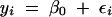
where y_i are the phenotypes, β₀ and β₁ are regression coefficients, and ε_i are normal errors. The index i runs through all individuals in the cross(es). We allow the QTL, represented by genotypes Q_i, to scan over a grid of locations covering the genome and plot a LOD score to summarize the evidence for a QTL at each location. The LOD score, in this case, is the difference in the log₁₀ likelihood values between models (1) and (2), where the individual model likelihoods are maximized with respect to the regression coefficients. If, instead of maximizing, we average over β_j with respect to a Bayesian prior distribution, we obtain the log posterior density of the QTL location (Sen and Churchill 2001). Note that Q_i is treated as a “dummy variable.” For a backcross, Q_i may be coded simply as 0 or 1 but for an intercross, Q_i will be represented by two indicator variables and β₁ will have two components. This convention helps us to avoid unnecessarily complicated notation. The actual states of the genotypes represented by Q_i cannot be observed directly. These must be inferred from marker data and phenotype values. Proper analysis requires that the QTL genotypes should be treated as missing data and an EM, imputation, or other “missing data” algorithm (Schafer 1997) should be used to compute the maximized likelihood. The problem of constructing missing data algorithms for QTL analysis has been thoroughly addressed (Lander and Botstein 1989; Kao and Zeng 1997; Sen and Churchill 2001). Thus, we can focus on the statistical model linking genotype to phenotype without having to worry about the details of the computations.

The simple genome scan explicitly assumes that a single QTL is affecting the phenotype. In general a phenotype may be influenced by multiple QTL as well as by factors such as sex or treatment variables and interactions among any of these. How do we go beyond simple genome scans to incorporate a richer class of models in our search for QTL?

First consider the introduction of a covariate into a genome scan. Including a term for an additive covariate in each of models (1) and (2) we obtain the pair of linear models:

3

4

A genome scan based on the LOD score contrasting models (3) and (4) accounts for the effects of a covariate that may be a factor (such as sex) or a continuous covariate (such as body weight) that has an additive effect on the average phenotypic value. Multiple covariates can be included and QTL at fixed, unlinked locations can be included as covariates in a scan.

The QTL effect may depend on the state of a covariate. For example, a QTL may have an effect only in male mice in a cross that includes both sexes. To model this we include a QTL-by-covariate interaction term in the linear model:

5

To make inferences about covariate-dependent QTL effects, one must consider all three models, (3), (4), and (5). One reasonable approach is to scan the QTL position computing the LOD score contrasting model (5) with model (3). This provides a peak LOD score at the most likely position of the QTL. We then compute the change in likelihood between models (4) and (5) at the peak position obtained under model (5) as a test for the QTL-by-covariate interaction.

Genome scans for combined crosses:

Suppose we are interested in QTL that may be shared across two or more inbred line crosses and we have recoded the alleles as described above. We can employ the set of linear models (3), (4), and (5) to construct genome scans. In this case X_i is a cross indicator. Model (3) represents the null hypothesis of no QTL and model (4) represents a shared QTL. Including cross (X_i) as an additive covariate accounts for differences in the average phenotype between crosses but the QTL effect is assumed to be the same in all crosses. The LOD score contrasting models (3) and (4) is used to construct a genome scan (Comb1) for shared QTL.

The cross term in these models plays the same role as the polygene term in Liu and Zeng (2000). In a single inbred line cross, all individual progeny are equi-correlated and the correlation structure can be safely ignored. When multiple crosses are combined this is no longer true and the cross term is important to avoid bias in estimation and to obtain a powerful test with the correct type I error level (Zou et al. 2001). This covariance interpretation suggests that it may be reasonable to treat cross as a random term in a mixed linear model. However, we are looking at a small number of crosses and these crosses are the focus of our inference. Thus, we have chosen to treat cross as a fixed effect following the recommendation of Zou et al. (2001).

QTL effects may vary from cross to cross. For example, the QTL may be absent in one cross but present in another. Model (5) includes a QTL-by-cross interaction term that allows each genotype in each cross to have its own effect. This recapitulates the multiple-allele model and is essentially identical to the multiple-allele model of Liu and Zeng (2000). When some of the crosses share strains in common, model (5) is slightly more general than the multiple-allele model. For example, we could have strain P contributing a high allele in cross P × I and a low allele in cross P × D. The LOD score contrasting model (5) and model (3) can be used to construct a genome scan (Comb2) for QTL that show any pattern of effects, not necessarily the pattern implied by the binary encoding of alleles.

The problem of establishing significance levels for genome scans has been extensively studied. Our preferred method is to use permutation analysis (Churchill and Doerge 1994). When performing the permutations, it is important to retain the pairing of phenotypes and covariates (e.g., cross and sex). If the X chromosome is scanned, permutations should be stratified by sex to avoid “illegal” genotypes. Stratification by cross preserves the covariance structure of the combined crosses. A combined-cross analysis involves construction of several genome scans. The scans are not independent and we have applied genome-wide adjusted thresholds on a per-scan basis. The significant QTL are selected using stringent criteria from the combined scans (Comb1 and Comb2). The individual cross scans are used primarily for decoding the QTL allelic distributions and may be interpreted more liberally using a suggestive threshold for significance.

Testing cross-specific QTL:

If a QTL is detected in the genome scan using model (5), we can test for cross-specific effects by computing the change in LOD score between models (5) and (4) at the peak location of the model (5) (Comb2) genome scan. We refer to this test statistic as ΔLOD1. It will be large for any QTL that deviates from the predicted pattern of allele effects.

We use the asymptotic chi-square distribution of the likelihood-ratio statistic to establish the significance of ΔLOD1. We have not applied any multiple test correction because the test is carried out at a single, fixed locus. To convert a LOD score to the chi-square scale, compute χ² = 2 ln(10^LOD), where ln is the natural logarithm. The degrees of freedom for the chi square are determined by the difference in the number of free parameters between the models being compared. In the example below, ΔLOD1 has 6 d.f. and the 0.05 LOD critical value is 2.73.

Resolving linked QTL:

When we observe coincident QTL in two or more crosses it is always possible that these are distinct QTL that have colocalized by chance. This situation could be described by a model,

6

with two cross-specific QTL. We can fit this multiple-QTL model using a simultaneous scan of all locus pairs on a single chromosome. The maximum LOD obtained in the pairwise scan can be compared to the maximum LOD obtained in the single-locus scan using model (5). The difference in log₁₀ likelihoods provides a test (ΔLOD2) for two QTL. This approach may be modified depending on the circumstances. For example, if we suspect that there are two linked QTL, one shared and one cross-specific, we could drop one of the QTL-by-cross interaction terms from model (6). It is also possible to scan a chromosome using a three-QTL model.

Significance of ΔLOD2 can establish the presence of multiple linked QTL that might otherwise appear to be a single shared QTL. The computation involves scanning the QTL locations under both models. Hence multiple testing is an issue. The comparison is made between two models with different numbers of QTL whose locations are free to vary. This leads to a situation where the usual assumptions of likelihood-ratio testing do not apply (Self and Liang 1987) and we cannot rely on standard asymptotic results. Furthermore, the null model [model (5)] in this test includes a QTL so it is not obvious how permutation analysis can be applied. Therefore, we simulated data from a single-QTL model with effect sizes estimated from the data using model (5) and computed ΔLOD2 1000 times to establish the critical values. These appear to depend on both the QTL effect size and the chromosome size but, for the cases considered here, ΔLOD2 values that exceed 4.5 may be regarded as significant evidence for two linked QTL. It is important to emphasize that failure to achieve significance does not conclusively establish that there is only a single QTL. Linked QTL can be difficult to separate. Thus, even a modestly significant result should be regarded as an indication that multiple loci may be involved, because of the implications for the further steps in identifying the genes, e.g., breeding congenic mouse strains or analysis of candidate genes.

RESULTS

Genome-wide analysis of HDL QTL:

We combined the data from four crosses (P × I, P × D, C × D, and C × S) and constructed a cross indicator. Binary allelic states were coded on the basis of the parental phenotypes as described above. We then carried out a combined-cross analysis to identify QTL associated with HDL cholesterol (square-root transformed). Figure 3 summarizes the genome-wide scans on the individual and combined data crosses. The combined-cross genome scan (Comb2) identified four significant QTL (chromosomes 1, 2, 4, and 6) and two suggestive QTL (chromosomes 5 and 11). Figure 4 shows allele-effect plots for each of these QTL in each cross. Test statistics and support intervals are summarized in Table 2. Among the QTL detected, chromosome 4 stands out as the most significant and it appears to be the only QTL shared among all four crosses. In the follow sections we describe the local analysis for each of these six QTL regions in order of their significance. In addition there is suggestive evidence for QTL on each of chromosomes 7, 9, 15, 17, and 18 in at least one of the crosses. However, we did not investigate these loci further.

Figure 3.—

Genome scans for individual and combined-cross analyses. The y-axis represents the LOD score. Individual crosses are as labeled. Comb1 is the model (3) vs. model (4) LOD score. Comb2 is the model (3) vs. model (5) LOD score. Significance thresholds are 0.05 and 0.63 levels (based on 1000 permutations) and are indicated by dashed lines.

Figure 4.—

Allele-effect plots. Rows in the grid show QTL peak locations and columns show crosses. Shaded parts indicate evidence for a QTL in the individual crosses. The y-axis on each part is square root of HDL cholesterol centered on the cross-specific mean. Error bars are ±1 SE.

TABLE 2.

HDL QTL summary

Chr	P × I	P × D	C × D	C × S	Comb1	Comb2	ΔLOD1	ΔLOD2
1	5.72, 86 cM   (70–94)	4.82, 76 cM   (66–98)	1.23, 86 cM,   NS	10.51, 86 cM   (76–90)	9.28*	3.83
2	5.68, 48 cM   (40–56)	1.66, 46 cM,   NS	9.21, 48 cM   (42–56)	7.60*	3.09
4	3.41, 24 cM   (10–44)	3.17, 20 cM   (8–34)	6.86, 20 cM   (10–34)	3.65, 22 cM   (0–36)	16.34, 22 cM   (16–28)	18.51, 22 cM   (16–28)	2.18	3.49
5	5.51, 0 cM   (0–10)	0.86, 0 cM,   NS	6.00, 2 cM   (0–14)	5.18*	4.25
6	4.25, 68 cM   (42–74)	4.06, 68 cM   (48–74)	9.67, 68 cM   (46–74)	5.63*	4.54*
11	3.23, 28 cM   (10–54)	2.91, 34 cM   (6–46)			2.83, 26 cM   (14–44)	5.80, 20 cM   (12–48)	3.19*	4.05

LOD score, peak position, and support intervals are listed for significant or suggestive QTL found in this study. Significant QTL are shown in italics. Comb1 indicates the combined analysis assuming a shared QTL in all crosses. The LOD score is based on model (4) vs. model (3) and binary encoding PC:IDS. Comb2 indicates the combined-cross analysis with cross-specific effects [model (5) vs. model (3)]. The ΔLOD1 test is used to detect cross-specific effects [model (5) vs. model (4)] at the peak location of the Comb2 scan. Significant (P < 0.05) values of ΔLOD1 are >2.73. The ΔLOD2 test is used to detect multiple linked QTL [model (6) vs. model (5)] on a chromosome. Significant values of ΔLOD2 (P < 0.05) are >4.5. *P < 0.05. Chr, chromosome.

Chromosome 4:

Chromosome 4 presents a significant QTL in the combined-cross scans and it is significant or nearly so in each of the individual crosses (Figure 3). In each case, the LOD curve shows a single quadratic peak centered on the region around 20–25 cM. The support intervals in individual crosses (Figure 5 and Table 2) are 20 to 30 cM in width. Allele-effect plots (Figure 4) show that in each cross the “B” allele is associated with high HDL cholesterol levels. The test for cross-specific allele effects (ΔLOD1 = 2.18, P = 0.12) is consistent with a shared QTL. There is no evidence for multiple QTL in this region (ΔLOD2 = 3.49, NS). We conclude that the chromosome 4 locus is likely to represent a shared QTL with allelic distribution PC:IDS, consistent with parental phenotypes. The combined-cross support interval based on the shared-QTL model (Comb1) is 16–28 cM. This represents a substantial narrowing of the QTL region to ∼10 cM.

Figure 5.—

Localization of the chromosome 4 QTL for four individual crosses and combined crosses. The QTL alleles are encoded as PC:IDS. The solid curve is the LOD score and the dashed curve is the posterior probability density of the QTL location. Triangles indicate markers that were genotyped in the individual crosses and the 2-cM-spaced tick marks indicate the location of imputed pseudomarkers. Shaded boxes delimit 95% support intervals for the QTL location.

Chromosome 1:

Chromosome 1 presents a significant LOD score in the region around 86 cM in the combined-cross genome scan (Comb2) and significant peaks in crosses P × D and C × S. The C × S LOD curve is unimodal with a peak at 76 cM. The P × D LOD curve also has a peak at 86 cM but it is bimodal with a minor peak at 50 cM. The test for cross-specific effect (ΔLOD1 = 7.8, P < 0.001) indicates that this QTL is not consistent with the binary encoding. On the basis of the assumption of a single shared QTL, the most likely biallelic distribution is PIS:DC. Higher HDL levels are associated with the P and S alleles (Figure 4).

We carried out a secondary analysis using only crosses P × D and C × S and encoded the alleles as PS:DC. For this analysis, ΔLOD1 = 0.06 (P = 0.99), which is consistent with a shared QTL. The test for two QTL (ΔLOD2 = 1.84, NS) does not suggest the presence of multiple QTL. However, there are a number of reasons why we should remain open to the possibility of multiple linked QTL in this region. First, we note that the peak LOD scores in the individual crosses differ in location by 10 cM. Second, the combined-cross support interval (68–102 cM; Figure 6, Comb1) is not substantially narrower than the interval obtained by analyzing cross P × D alone. Finally, the combined LOD curve is not unimodal. In a separate study Wang et al. (2004) have shown that a polymorphism in Apoa2 (at 92 cM) is responsible for the C × S QTL. Strains P and D do not differ at the causal polymorphism in Apoa2. The most likely candidate for the P × D QTL is an uncharacterized locus that lies 6 cM proximal to Apoa2 (B. Paigen, personal communication). This example underscores the importance of critically examining the LOD curves in a combined-cross analysis and the care that must be taken in the interpretation of nonsignificant test results.

Figure 6.—

Posterior density of chromosome 1 (left) and chromosome 11 (right) QTL locations after recoding as shared QTL on a subset of the crosses. QTL alleles on chromosome 1 are encoded as PS:IDC. QTL alleles on chromosome 11 are encoded as P:IDCS. Details are as in Figure 5.

Chromosome 2:

Chromosome 2 presents a significant peak at 48 cM in the combined-cross genome scan (Figure 3, Comb2). A similar peak occurs in cross C × D but there is no evidence for a chromosome 2 QTL in any of the other crosses. The test for cross-specific QTL (ΔLOD1 = 7.60, P < 0.001) is significant. Effect plots suggest that a recessive D allele is associated with high HDL in cross C × D. We conclude that the chromosome 2 QTL is cross-specific with allele distribution PID:CS. The QTL is segregating in only one cross so there is no further advantage to combining cross data in this case. The QTL support interval based on cross C × D is 40–56 cM.

Chromosome 6:

Chromosome 6 presents a significant peak at 68 cM in the combined-cross scan (Figure 3, Comb2). Significant peaks are also in the shared-QTL scan (Figure 3, Comb1) and in cross C × D. A suggestive peak occurs in cross C × S at 70 cM. In crosses P × I and P × D, chromosome 6 does not reach the suggestive level. The cross-specific QTL test (ΔLOD1 = 5.63, P < 0.001) is significant and the allele-effect plots (Figure 4) confirm that chromosome 6 is not a shared QTL. We conclude that the chromosome 6 QTL has allele distribution PIDS:C, where the C allele is associated with lower HDL. The alternative coding PIC:DS cannot be definitively ruled out in light of the consistent but weak evidence for a QTL present in cross P × D.

Chromosome 5:

Chromosome 5 presents a suggestive peak at 0 cM in the combined-cross scan (Comb2) and a significant peak in cross P × I. The cross-specific QTL test (ΔLOD1 = 5.2, P < 0.001) is significant and is confirmed by the allele-effect plots (Figure 4). We conclude that chromosome 5 allele distribution is I:PDCS with the I allele contributing an additive effect associated with lower HDL levels. As this QTL appears only in cross P × I, there is no advantage to combining data. The chromosome 5 support interval based on cross P × I is 0–10 cM.

Chromosome 11:

Chromosome 11 presents suggestive peaks at 26 and 20 cM, respectively, in the combined-cross scans (Figure 3). The cross-specific test (ΔLOD1 = 3.19, P = 0.023) is only marginally significant. The individual cross scans show peaks that are nearly significant in crosses P × I and P × D whereas the crosses C × S and C × D present no evidence for a QTL on chromosome 11. Together with the allele effects (Figure 4), these observations suggest that the chromosome 11 QTL most likely has a P:IDCS allele distribution.

On this assumption, we recoded the alleles and combined crosses P × I and P × D. The cross-specific test in this case (ΔLOD1 = 0.57, P = 0.85) is consistent with a shared QTL and there is no evidence for multiple QTL (ΔLOD2 = 1.72, NS). The support interval based on the shared-QTL model (Figure 6, Comb1) spans the region from 20 to 44 cM, still quite broad but narrower than the individual cross support intervals.

Pairwise genome scans identified an interaction between loci on chromosomes 4 and 11. A significant LOD peak was detected in cross C × D at chromosome 4 at 24 cM and chromosome 11 at 20 cM. The LOD for a two-QTL model with interaction is 12.08 (P < 0.05, genome-wide adjusted). The component of the LOD attributable to interaction alone is 4.53 (P = 0.0003, unadjusted). An allele-effect plot for the interaction is shown in Figure 7. The pattern of the interaction suggests that a homozygous CC genotype on chromosome 11 is required for the effect of chromosome 4 to be expressed in this genetic background.

Figure 7.—

Interacting allele effects between the chromosome 4 and chromosome 11 QTL in cross C × D. The two leftmost parts show the main effects of QTL on chromosomes 4 and 11 and the rightmost part shows their joint effect. The vertical scale is the square root of HDL. Points indicate the mean phenotype for each genotypic group and the bar indicates 95% confidence intervals for the mean (±2 SE).

A second interacting locus pair was detected in cross C × S between two loci on chromosome 11 at 10 and 25 cM. The two QTL plus interaction LOD score is 14.27 (P < 0.05, genome-wide adjusted) and the component of the LOD attributable to the interaction is 12.86 (P < 0.001). Tightly linked and interacting QTL are always suspect. Closer inspection of this interaction revealed that the mouse with highest HDL level among all crosses (HDL = 378 mg/dl, Figure 1) has a pair of recombination events on proximal chromosome 11 and this is the only mouse with genotype (CC/SS = AA/BB) at these loci. In light of the singular nature of this event, we are inclined to disregard the finding. However, it does hint at the possibility that the suggestive QTL region on chromosome 11 region may harbor a more complex genetic architecture than we can resolve with these crosses.

DISCUSSION

Linear models are implicitly used in genome scans and in most QTL analyses. However, the central role of linear models in QTL analysis is often not recognized or made explicit. New software tools are available that enable an analyst to carry out explicit and general linear modeling of QTL (R/qtl, Broman et al. 2003; pseudomarker, Sen and Churchill 2001). These tools present an opportunity to explore the architecture of complex traits in greater depth than ever before. Combined-cross analysis is just one of many possible applications that can be developed.

The binary encoding strategy described here is especially promising for application using the common strains of inbred laboratory mice due to the effectively biallelic nature of many polymorphic loci (Wade et al. 2002). Combining data from two or more inbred line crosses on the basis of a binary allele-effects model may be applicable to other diploid organisms with similar breeding history to the laboratory mouse. The key assumption is that there is a substantial prior probability that two common QTL alleles will be shared among the parental lines.

A combined-cross analysis may be conducted as a post hoc meta-analysis of existing data. However, there may be some advantages to planning multiple-cross mapping experiments. Eliminating potential confounding factors and conducting the crosses in a controlled, uniform environment minimizes gene-by-environment interactions and increases the likelihood that shared QTL will be detected. There are tradeoffs to consider. A typical mapping study is constrained by the total number of individuals that can be generated and phenotyped. Generating progeny from multiple strains offers an advantage in that more QTL can be detected. However, as we have seen in the example here, some of these QTL will be segregating in only a subset of the total progeny and this will reduce the power compared to a single-cross study of the same total size. For example, four crosses of 250 individuals each should provide reasonable power to detect QTL that account for 5–10% of the total variance even if allelic differences are limited to just one of the crosses. On the other hand, a single cross with 1000 progeny should have power to detect QTL with effect sizes on the order of 2% of total variance but fewer loci are likely to be segregating.

The advantages of combined-cross analysis are increased power for detecting QTL and improved localization of shared QTL. As demonstrated in our example, these gains may be modest and will not by themselves provide gene-level resolution of QTL. We propose that combined-cross analysis could serve as a preliminary step to QTL localization by haplotype analysis (Wade et al. 2002; Wiltshire et al. 2003). A combined-cross analysis can (usually) determine the parental allelic states on the basis of the pattern of QTL found in the individual crosses. Knowledge of the parental alleles can be leveraged to achieve very high resolution of QTL location by comparing the haplotypes of the parental lines in the QTL support interval to the predicted the biallelic pattern. In many instances this could provide resolution of a QTL to a very small and manageable number of genes for follow-up studies. Some allowance must be made for the existence of third alleles in crosses that include wild-derived mouse strains. In our example, the CAST/Ei strain could potentially contribute alleles that are distinct from the other, standard inbred strains.

It is interesting to note that most of the QTL defined in our example were not consistent with the pattern of allelic effect predicted by the parental phenotypes. Indeed, each of our QTL showed a distinct distribution across the parental lines. This should not be surprising, as there is no reason (e.g., selection) that HDL-related QTL should show clustering of allelic types within strains. A mixture of alleles is likely to contribute to buffering of important phenotypes. The common observation of transgressive segregation in intercross populations suggests that parental lines with low phenotypes can often contribute high alleles and vice versa. We conclude that efforts to map QTL solely on the basis of the parental strain phenotypes (e.g., “in silico mapping”; Grupe et al. 2001) are likely to miss many important features of the genetic architecture of complex traits.

The results obtained with the test for multiple QTL ΔLOD2 in this study were somewhat disappointing. A previous study using an advanced intercross design (Wang et al. 2003) suggested that chromosomes 1 and 5 are likely to harbor multiple HDL QTL. However, as these QTL appear to be tightly linked in coupling phase, the combined intercrosses do not provide sufficient resolution to separate the effects. The evidence for multiple linked QTL on chromosome 6 is consistent with our previous analysis of this QTL (Lyons et al. 2003a). In other studies (M. A. Lyons, R. Li, G. A. Churchill and B. Paigen, unpublished results) we have successfully resolved multiple linked QTL with unambiguously significant ΔLOD2 results. For the purpose of combining crosses we recommend liberal interpretation of this test and careful attention to other sources of evidence. In the combined-cross analysis we make an assumption regarding the biallelic nature of QTL that occur in more than one cross. These assumptions may not be always correct but they move us forward. The conclusions of a combined-cross analysis are intended to provide guidance in follow-up studies. The possibility of multiple linked QTL and multiple alleles at a single locus must always be kept in mind.

In conclusion, we have described and demonstrated the utility of combining multiple crosses for QTL mapping. This technique offers an opportunity to better utilize existing data from resource-intensive breeding crosses and should have immediate benefits for QTL analysis studies in the laboratory mouse. Application of the analysis techniques described here should improve the power and resolution of QTL studies and will provide further insights into the genetic determinants of complex phenotypes.

References

- Abiola, O., J. M. Angel, P. Avner, A. A. Bachmanov, J. K. Belknap et al., 2003. The nature and identification of quantitative trait loci: a community's view. Nat. Rev. Genet. 4: 911–916. [DOI] [PMC free article] [PubMed] [Google Scholar]
- Beck, J. A., S. Lloyd, M. Hafezparast, M. Lennon-Pierce, J. T. Eppig et al., 2000. Genealogies of mouse inbred strains. Nat. Genet. 24: 23–25. [DOI] [PubMed] [Google Scholar]
- Bonhomme, F., 1986. Evolutionary relationships in the genus Mus. Curr. Top. Microbiol. Immunol. 127: 19–34. [DOI] [PubMed] [Google Scholar]
- Broman, K. W., H. Wu, S. Sen and G. A. Churchill, 2003. R/qtl: QTL mapping in experimental crosses. Bioinformatics 19: 889–890. [DOI] [PubMed] [Google Scholar]
- Churchill, G. A., and R. W. Doerge, 1994. Empirical threshold values for quantitative trait mapping. Genetics 138: 963–971. [DOI] [PMC free article] [PubMed] [Google Scholar]
- Glazier, A. M., J. H. Nadeau and T. J. Aitman, 2002. Finding genes that underlie complex traits. Science 298: 2345–2349. [DOI] [PubMed] [Google Scholar]
- Grupe, A., S. Germer, J. Usuka, D. Aud, J. K. Belknap et al., 2001. In silico mapping of complex disease-related traits in mice. Science 292: 1915–1918. [DOI] [PubMed] [Google Scholar]
- Haley, C., and S. A. Knott, 1992. A simple regression method for mapping quantitative trait loci in line crosses using flanking markers. Heredity 69: 315–324. [DOI] [PubMed] [Google Scholar]
- Hitzemann, R., B. Malmanger, C. Reed, M. Lawler, B. Hitzemann et al., 2003. A strategy for the integration of QTL, gene expression, and sequence analyses. Mamm. Genome 14: 733–747. [DOI] [PubMed] [Google Scholar]
- Jannink, J. L., and R. Jansen, 2001. Mapping epistatic quantitative trait loci with one-dimensional genome searches. Genetics 157: 445–454. [DOI] [PMC free article] [PubMed] [Google Scholar]
- Jansen, R. C., and P. Stam, 1994. High resolution of quantitative traits into multiple loci via interval mapping. Genetics 136: 1447–1455. [DOI] [PMC free article] [PubMed] [Google Scholar]
- Kao, C. H., and Z. B. Zeng, 1997. General formulas for obtaining the MLEs and the asymptotic variance-covariance matrix in mapping quantitative trait loci when using the EM algorithm. Biometrics 53: 653–665. [PubMed] [Google Scholar]
- Khanuja, B., Y. C. Cheah, M. Hunt, P. M. Nishina, D. Q. Wang et al., 1995. Lith1, a major gene affecting cholesterol gallstone formation among inbred strains of mice. Proc. Natl. Acad. Sci. USA 92: 7729–7733. [DOI] [PMC free article] [PubMed] [Google Scholar]
- Korstanje, R., and B. Paigen, 2002. From QTL to gene: the harvest begins. Nat. Genet. 31: 235–236. [DOI] [PubMed] [Google Scholar]
- Lander, E., and L. Kruglyak, 1995. Genetic dissection of complex traits: guidelines for interpreting and reporting linkage results. Nat. Genet. 11: 241–247. [DOI] [PubMed] [Google Scholar]
- Lander, E. S., and D. Botstein, 1989. Mapping Mendelian factors underlying quantitative traits using RFLP linkage maps. Genetics 121: 185–199. [DOI] [PMC free article] [PubMed] [Google Scholar]
- Liu, Y., and Z. B. Zeng, 2000. A general mixture model approach for mapping quantitative trait loci from diverse cross designs involving multiple inbred lines. Genet. Res. 75: 345–355. [DOI] [PubMed] [Google Scholar]
- Lyons, M. A., H. Wittenburg, R. Li, K. A. Walsh, G. A. Churchill et al., 2003. a Quantitative trait loci that determine lipoprotein cholesterol levels in DBA/2J and CAST/Ei inbred mice. J. Lipid Res. 44: 953–967. [DOI] [PubMed] [Google Scholar]
- Lyons, M. A., H. Wittenburg, R. Li, K. A. Walsh, M. R. Leonard et al., 2003. b New quantitative trait loci that contribute to cholesterol gallstone formation detected in an intercross of CAST/Ei and 129S1/SvImJ inbred mice. Physiol. Genomics 14: 225–239. [DOI] [PubMed] [Google Scholar]
- Nadeau, J. H., and W. N. Frankel, 2000. The roads from phenotypic variation to gene discovery: mutagenesis versus QTLs. Nat. Genet. 25: 381–384. [DOI] [PubMed] [Google Scholar]
- Paigen, K., 1995. A miracle enough: the power of mice. Nat. Med. 1: 215–220. [DOI] [PubMed] [Google Scholar]
- Park, Y. G., R. Clifford, K. H. Buetow and K. W. Hunter, 2003. Multiple cross and inbred strain haplotype mapping of complex-trait candidate genes. Genome Res. 13: 118–121. [DOI] [PMC free article] [PubMed] [Google Scholar]
- Rebai, A., B. Goffinet and B. Mangin, 1994. Approximate thresholds of interval mapping tests for QTL detection. Genetics 138: 235–240. [DOI] [PMC free article] [PubMed] [Google Scholar]
- Schafer, J., 1997 Analysis of incomplete multivariate data. Monographs on Statistics and Applied Probability 72. Chapman & Hall, London.
- Self, S. G., and K-Y Liang, 1987. Asymptotic properties of maximum likelihood estimators and likelihood ratio tests under nonstandard conditions. J. Am. Stat. Assoc. 82: 605–610. [Google Scholar]
- Sen, S., and G. A. Churchill, 2001. A statistical framework for quantitative trait mapping. Genetics 159: 371–387. [DOI] [PMC free article] [PubMed] [Google Scholar]
- Silver, L., 1995 Mouse Genetics. Oxford University Press, Oxford.
- Sugiyama, F., G. A. Churchill, D. C. Higgins, C. Johns, K. P. Makaritsis et al., 2001. Concordance of murine quantitative trait loci for salt-induced hypertension with rat and human loci. Genomics 71: 70–77. [DOI] [PubMed] [Google Scholar]
- Wade, C. M., E. J. Kulbokas, III, A. W. Kirby, M. C. Zody, J. C. Mullikin et al., 2002. The mosaic structure of variation in the laboratory mouse genome. Nature 420: 574–578. [DOI] [PubMed] [Google Scholar]
- Walling, G. A., P. M. Visscher, L. Andersson, M. F. Rothschild, L. Wang et al., 2000. Combined analysis of data from quantitative trait loci mapping studies: chromosome 4 effects on porcine growth and fatness. Genetics 155: 1369–1378. [DOI] [PMC free article] [PubMed] [Google Scholar]
- Wang, X., I. Le Roy, E. Nicodeme, R. Li, R. Wagner et al., 2003. Using advanced intercross lines for high-resolution mapping of HDL cholesterol quantitative trait loci. Genome Res. 13: 1654–1664. [DOI] [PMC free article] [PubMed] [Google Scholar]
- Wang, X., R. Korstanje, D. Higgins and B. Paigen, 2004. Haplotype analysis in multiple crosses to identify a QTL gene. Genome Res. 14: 1767–1772. [DOI] [PMC free article] [PubMed] [Google Scholar]
- Wittenburg, H., M. A. Lyons, R. Li, G. A. Churchill, M. C. Carey et al., 2003. Primary roles of FXR and ABCG5/8 in cholesterol gallstone susceptibility in inbred mice: evidence from quantitative trait locus analysis. Gastroenterology 125: 868–881. [DOI] [PubMed] [Google Scholar]
- Wiltshire, T., M. T. Pletcher, S. Batalov, S. W. Barnes, L. M. Tarantino et al., 2003. Genome-wide single-nucleotide polymorphism analysis defines haplotype patterns in mouse. Proc. Natl. Acad. Sci. USA 100: 3380–3385. [DOI] [PMC free article] [PubMed] [Google Scholar]
- Zeng, Z-B., 1994. Precision mapping of quantitative trait loci. Genetics 136: 1457–1468. [DOI] [PMC free article] [PubMed] [Google Scholar]
- Zou, F., B. S. Yandell and J. P. Fine, 2001. Statistical issues in the analysis of quantitative traits in combined crosses. Genetics 158: 1339–1346. [DOI] [PMC free article] [PubMed] [Google Scholar]