Modeling Quantitative Trait Loci and Interpretation of Models

Abstract

A quantitative genetic model relates the genotypic value of an individual to the alleles at the loci that contribute to the variation in a population in terms of additive, dominance, and epistatic effects. This partition of genetic effects is related to the partition of genetic variance. A number of models have been proposed to describe this relationship: some are based on the orthogonal partition of genetic variance in an equilibrium population. We compare a few representative models and discuss their utility and potential problems for analyzing quantitative trait loci (QTL) in a segregating population. An orthogonal model implies that estimates of the genetic effects are consistent in a full or reduced model in an equilibrium population and are directly related to the partition of the genetic variance in the population. Linkage disequilibrium does not affect the estimation of genetic effects in a full model, but would in a reduced model. Certainly linkage disequilibrium would complicate the detection of QTL and epistasis. Using different models does not influence the detection of QTL and epistasis. However, it does influence the estimation and interpretation of genetic effects.

MANY quantitative genetics publications (e.g., Falconer and Mackay 1996) use the following model to interpret genetic effects between genotypes AA, Aa, and aa in one locus:

In this model, a is the additive effect defined as half of the difference between the two homozygote genotypic values, d is the dominance effect defined as the difference between the heterozygote genotypic value and the mean homozygote genotypic value, and μ is a constant. In this way, the genetic effects are defined only as a function of genotypic values. This is in contrast to a Fisherian model, where the genetic effects are defined specifically in reference to a population, usually an equilibrium population with specified allelic frequencies. The allelic substitution effect in a Fisherian model is traditionally called the average effect. As explained by Falconer and Mackay (1996)(p. 112), “average effects depend on the genotypic values, a and d as previously defined, and also on the gene frequencies. Average effects are therefore properties of populations as well as of the genes concerned.”

A similar argument has been made for epistasis (Cheverud and Routman 1995). On the one hand, we have the model proposed by Hayman and Mather (1955) and discussed in length in Mather and Jinks (1982), which is a direct extension of the above model to two loci. On the other hand, we have the model proposed by Cockerham (1954) following Fisher (1918) and a specific simplified model for an F₂ population proposed by Anderson and Kempthorne (1954). The model proposed by Cheverud and Routman (1995) is, however, somewhat different.

We seek to compare these models on the meaning and interpretation of genetic effects, including epistatic effects, particularly in reference to QTL mapping analysis. Previously, Van Der Veen (1959) gave a comparison of the model by Hayman and Mather (1955), called by Van Der Veen (1959) as the F_∞-metric model; the model by Anderson and Kempthorne (1954), called the F₂-metric model; and another model, called the mixed-metric model. However, the comparison by Van Der Veen (1959) was restricted to the transformation of parameter values from one model to another.

The issue is actually more than whether a model is defined on the basis of genotypic values only or also on the basis of allelic frequencies. Even if model parameters are defined only on the basis of genotypic values, there are many ways to define a QTL model, thus additive, dominance, and epistatic effects. The models compared by Van Der Veen (1959) are all based on genotypic values only, so to speak.

The purpose of modeling QTL, of course, is to provide a way to summarize and interpret the differences between the genotypic values and also the genetic variation observed in a study population. This can be facilitated if a model is consistent in the definition of the genetic effects in a full or reduced model with multiple loci under certain conditions.

Here we provide a framework to compare these models. All of these models are regression based and models differ by different specifications of the regressors related to additive and, particularly, dominance effects and thus to epistatic effects as well. In this way, the similarities and differences between the models become apparent. We discuss and compare the meaning of genetic effects defined in different models in different situations with respect to one, two, or multiple loci. We also discuss potential problems in using some models in a segregating population for QTL analysis. Last, we discuss how to estimate and interpret estimates of genetic effects in a population with loci in linkage disequilibrium.

MODELS

F_∞ model—traditional model: The regression equation for this model is

1

with

2

where a and d are additive and dominance effects of QTL and w and v are the corresponding genetic-effect design variables. With three genotypic values and three parameters, there is a unique solution for the parameter values. We use matrix notation to give this solution for reasons that will later become apparent.

Let us define

Then

represents

3

Multiplying on both sides by the inverse of the genetic-effect design matrix, S⁻¹_F∞·A, leads to

4

Here the departure point (μ) is defined as the mean of two homozygote genotypic values. This corresponds to the mean in an F_∞ population, a population continuously selfed for many generations starting from an F₁. For this reason, Van Der Veen (1959) called it the F_∞-metric model. We shorten it to the F_∞ model.

Recall that the additive effect a is defined as half of the difference between the homozygote genotypic values (G₂ and G₀) and that the dominance effect d is defined as the difference between the heterozygote genotypic value (G₁) and the mean of the homozygote genotypic values.

If the allelic frequency for allele A is 0.5, the expected value of w is zero. However, the expected value of v is not zero for any allelic frequency. This has implications for the definition and interpretation of additive and dominance effects with epistasis on two or more loci.

An extension of (1) to two loci with epistasis yields

5

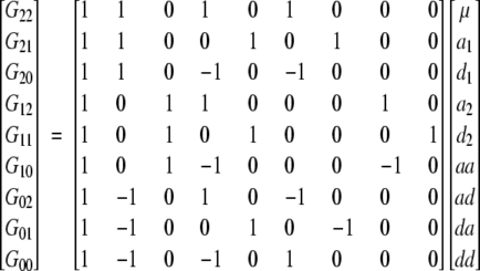
with w₁, v₁, w₂, and v₂ defined by (2) for loci 1 and 2, correspondingly. Excluding the additive and dominance effects for both loci, there are four epistatic (interaction) effects: the additive × additive effect (aa)₁₂ is associated with the product of additive-effect design variables w₁ and w₂, while the additive × dominance effect (ad)₁₂ is associated with the product of additive- and dominance-effect design variables w₁ and v₂, and so on.

Expressed in matrix notation, the F_∞ model takes the form

6

(Hayman and Mather 1955; Mather and Jinks 1982), or

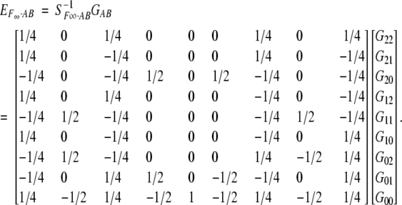
The unique solution for E_F∞·AB is

7

The departure point (μ) again is the unweighted (or equally weighted) mean of the homozygote genotypic values, still corresponding to the mean in an F_∞ population.

However, the additive and dominance effects for each locus in (7) are now defined with respect to the homozygote genotypes at the other locus. This is actually different from the definition at one locus in (4). When we use Equation 4 to define and estimate the additive and dominance effects for locus A, for example, the genotypes at locus B and other loci are not defined. Thus, both theoretically and practically, it means that the effects at locus A are defined with reference to genotypes at locus B and any other loci weighted by the genotypic frequencies in the application population.

For example, for only two loci A and B in linkage equilibrium in an F₂ population, the implied definition of a₁ and b₁ by (4) is

which is different from that in (7).

This is also the definition of the additive and dominance effects for two loci in linkage equilibrium without fitting epistatic effects,

So for the F_∞ model the additive and dominance effects are defined differently, depending on whether the epistatic effects are fitted in the model. This is because the F_∞ model is not an orthogonal model; i.e., the effects are not defined to be independent for loci even in a population with Hardy-Weinberg and linkage equilibrium. So even though the additive and dominance effects a and d for the F_∞ model are independent if there is Hardy-Weinberg equilibrium, the dominance effects and the dominance × dominance effect are not. This is because the mean of the dominance effect design variable in the F_∞ model, E(v₁) or E(v₂), is not scaled to zero and, as a result, there is a covariance between the dominance effects and the dominance × dominance interaction effect even for loci in equilibrium. So even when v₁ and v₂ are independent, which means E(v₁v₂) = E(v₁)E(v₂), however, .

Note that the genetic-effect design matrix for two loci, S_F∞·AB, is a direct product (Kronecker product) of two one-locus design matrices S_F∞·A and S_F∞·B with some columns rearranged to conform to the usual parameter order in E_F∞·AB. An important property for the direct product of matrices is that the inverse of the direct product of two square and nonsingular matrices is the direct product of the inverses of matrices.

Define this column-rearranged direct product by . It can be shown that , where ′ denotes transposition. In other words, S⁻¹_F∞·AB is a direct product of S⁻¹_F∞·A and S⁻¹_F∞·B with some rows rearranged correspondingly.

This operation is particularly useful for three or more loci. It applies to other models presented below as well. In all cases the inverse of the design matrix can be readily obtained.

F₂ model—orthogonal model for p = ¹/₂ in an equilibrium population:

The F₂ model is another popular model used in quantitative genetics analysis. This model is directly related to the least-squares model based on the orthogonal partition of genetic variance in an equilibrium population (Cockerham 1954). When the number of alleles at a locus is restricted to two and allelic frequency is set to one-half, the least-squares model is reduced to the F₂ model. For one locus, the model can also be specified as a regression model (1) by using the genetic-effect design variables

8

which result in

9

and

10

The difference between the F₂ and F_∞ models is that variable d in (8) is scaled to zero for allelic frequency one-half. The starting point (μ) is the mean genotypic value for an F₂ population. Thus the model is known as the F₂ model. This change in d does not alter the definition of additive and dominance effects in a one-locus model as a and d in (4) and (10) are the same. However, for two or more loci with epistasis, they are different.

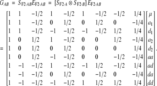
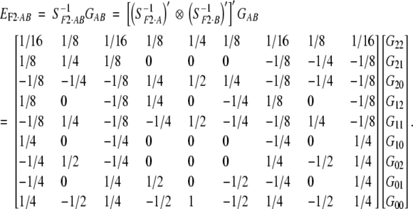
Extended to two loci, the F₂ model can still be expressed as (5) with (8) specifying corresponding genetic-effect design variables. In matrix notation,

11

and

12

This model directly follows Cockerham (1954) and first appeared in Anderson and Kempthorne (1954). Cockerham and Zeng (1996) used it for marker analysis in design III. The departure point (μ) is still the mean of an F₂ population in Hardy-Weinberg and linkage equilibrium.

In this case, since the means of the w and v variables are scaled to zero for the population, the effects in the model are all orthogonal for two or more loci in Hardy-Weinberg and linkage equilibrium. Thus the definitions of additive and dominance effects of each locus are consistent with respect to the other loci and with respect to the epistatic effects in an F₂ population. This means that the definition of a as well as d is the same whether or not other (independently segregating) loci or epistatic effects are fitted in the regression model. This orthogonal property is very important and useful for QTL analysis. In contrast, the F_∞ model does not have this property as explained above.

Note that the epistatic effects are defined in the same way for both the F₂ and F_∞ models. This is because the additive and dominance effects in S⁻¹_F2·A and S⁻¹_F∞·A for both models are defined in the same way. Thus when we take a direct product between additive and dominance effects of two loci, i.e., between the second and third rows of S⁻¹_F2·A and S⁻¹_F2·B or S⁻¹_F∞·A and S⁻¹_F∞·B, the epistatic effects are defined in the same way. However, when we take a direct product of the second and third rows of S⁻¹_F2·A or S⁻¹_F∞·A with the first row of S⁻¹_F2·B or S⁻¹_F∞·B, the additive and dominance effects for locus A become different for the two models due to the difference of the constant term of the one-locus models (the first row of S⁻¹_F2·B and S⁻¹_F∞·B). This is the reason that the specification of the constant term at one locus is important for the specification of the genetic effects at multiple loci. This argument extends to the specification of genetic effects at three or more loci through the direct product.

In comparison, the two-locus F_∞ model does look simpler and has thus been used extensively in inbred line and crossbred population mean analyses (e.g., Mather and Jinks 1982). However, the two-locus F_∞ model is not quite appropriate for use in QTL mapping analysis with epistasis in a segregating population, such as an F₂. With the dependence between the dominance effects and the dominance × dominance effect, the model makes the partition of genetic variance and interpretation of genetic effects with epistasis unnecessarily complicated. This problem would increase as more loci with epistasis are considered in a QTL mapping analysis. When analyzing the variance of cross populations, Mather and Jinks (1982)(Chap. 7) actually converted the F_∞ model parameters to the F₂ model parameters for analysis and interpretation.

For more discussion on a comparison of the two models, see Van Der Veen (1959) and Kao and Zeng (2002). Van Der Veen (1959) also discussed another model, called the mixed-metric model. It is just a mixture of the F₂ and F_∞ models—using the dominance effects from the F_∞ model and others from the F₂ model. This mixed-metric model behaves basically like an F₂ model in terms of the estimation of genetic effects and is rarely used in QTL analysis. Many other specialized genetic models have also been proposed over the years for a variety of specialized populations and applications (e.g., Griffing 1956; Hayman 1957; Eberhart and Gardner 1966; Hill 1982).

The orthogonal property of the F₂ model applies only for loci with allelic frequencies of one-half and in Hardy-Weinberg and linkage equilibrium. The question then arises as to what model we might use for generalized allelic frequencies. Prior to addressing this question, we discuss another model proposed by Cheverud and Routman (1995) and Cheverud (2000).

Unweighted regression model:

Recently, Cheverud and Routman (1995) and Cheverud (2000) proposed a model, which is equivalent to the regression model with model design variables,

13

The specification of this model at one locus is

14

and

15

Extending it to two loci, we have

with

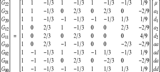16

and

with

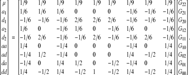17

Equation 17 is equivalent to Equations 4.8 and 4.9 of Cheverud (2000). This is the basis for our reconstruction of their model. There is a small, nonconsequential difference between the two presentations. The additive × dominance and dominance × additive effects differ by a factor of 2 and the dominance × dominance effect by a factor of ⁴/₉. [In presenting and discussing the model, Cheverud and Routman (1995) and Cheverud (2000) made a few errors, however. They mistakenly claimed, particularly in Cheverud (2000), that they followed the model in Falconer and Mackay (1996), which is an F_∞ model, and extended it to two loci. Equations 4.1–4.4 of Cheverud (2000) for one locus are not correct for the design variables provided. Equations 4.8 and 4.9 also do not follow Equation 4.7 and Table 4.1 of Cheverud (2000).]

Cheverud and Routman (1995) called it the unweighted regression (UWR) model because the departure point (μ) is the unweighted (or equally weighted) average of the nine genotypic values for two loci and the three genotypic values for one locus. In this model, the mean of the v variable is zero if the three genotypes have equal frequencies.

Again, the additive and dominance effects are defined in the same way as that of the F₂ and F_∞ models for one locus, but are different for two or more loci with epistasis due to the difference in the departure point. Also, the two-locus epistatic effects are defined in the same way as those in the F₂ and F_∞ models.

In introducing the UWR model, Cheverud and Routman (1995) made a few claims that are controversial. They tried to distinguish this model from the traditional least-squares model such as the F₂ model or the general two-allele model discussed below. They termed the UWR model as a “physiological genetic model” and its epistasis “physiological epistasis” because it does not depend on allelic frequencies. They referred to a model such as (11) or (18) below as a “statistical genetic model” and its epistasis as “statistical epistasis.” This physiological vs. statistical argument is unnecessary and potentially misleading. All these models are statistical descriptions of the differences and variation of different genotypic values in reference to different starting points or populations. If it is preferred, one can actually define numerous models that are independent of allelic frequencies. The F₂ model is an unweighted regression model based on gametes in linkage equilibrium, which also has a population interpretation.

However, the notion of a physiological model is intended to imply that the effects defined and estimated from it would be independent of the study population. Conceptually, the UWR model, like the F_∞ model, has a problem of multilocus inconsistency in practice, letting alone whether it is population independent. The effects defined in a two-locus system are different from those in a three-locus or multiple locus system. The genetic effects defined and estimated for pairwise loci separately are not the same as those for multiple loci. For example, applied to a mapping population, such as an F₂, for QTL analysis, the definitions of the additive and dominance effects for locus A when analyzed with locus B are actually different from those when analyzed with locus C for a two-locus analysis, because the effects depend on other loci fitted or not fitted in the model. The argument that the genetic effects estimated from a physiological model would be independent of the study population is wishful thinking.

Cheverud and Routman (1995) argued that the reason to separate physiological epistasis from statistical epistasis is that physiological epistasis also contributes to the additive and dominance genetic variances and statistical epistasis does not contain all of the physiological epistasis. This is a misunderstanding. It is known that the epistatic effects defined for a reference population, such as that with allelic frequencies one-half, would contribute positively or negatively to the additive and dominance genetic variances in a population where the allelic frequencies are not one-half, because the epistatic effects are higher-order statistics. This is similar to the situation in which the dominance effect defined for the allelic frequency one-half would contribute either positively or negatively to the additive effect and additive variance when the allelic frequency is not one-half, a justification for the general two-allele (G2A) model discussed below. An orthogonal model defined in one population would not necessarily be orthogonal in another population where the assumption for the orthogonality is violated. However, the situation for the F_∞ and UWR models is different. The models are not orthogonal in any relevant population for a quantitative genetics study. Thus when applied to a segregating population, such as an F₂ population, it is not surprising to find that the epistatic effects would contribute to the additive and dominance variances either positively or negatively. This is not because the F_∞ model or the UWR model naturally has more (or less) epistasis. The definition of epistasis for the F_∞ model and the UWR model is the same as that for the F₂ model. But the additive and dominance effects defined in those models are different and insufficient to account for the additive and dominance effects in the application population.

Also, as shown in the numerical example below, no matter what model is used, the variance explained by different models for the same analysis is actually the same, and no model in the current discussion can explain more epistasis than others. The conclusion by Routman and Cheverud (1997) that one can use the UWR model rather than other models to find more epistasis in an F₂ population is unfounded.

Incidentally, the regression model also provides a statistical way to analyze and test different genetic effects and variance components. If a model is orthogonal, the tests for different effects and variance components are independent. This is an advantage of the orthogonal model. Otherwise, a test for epistasis can still be performed by the comparison of test statistics between the full and reduced models with and without epistatic terms.

General two-allele model:

The orthogonal property of the F₂ model applies only to a population where allelic frequencies are one-half. In an association study in a natural population, allelic frequencies vary from marker to marker and from QTL to QTL. In terms of modeling QTL, it is desirable to have a model that has the orthogonal property for a variety of allelic frequency distributions.

Let us consider a locus of two alleles with allelic frequency p for A and 1 − p for a. Define an indicator variable for alleles by

where x is a standardized indicator variable with mean zero.

For regression model (1), we can use genetic-effect design variables

18

where x₁ and x₂ are for the two alleles in an individual. This is called the G2A model. Note that the v variable is proportional to the product of x₁ and x₂, which explains why the dominance effect is an interaction effect between the two alleles within a locus. Also note that when p = ¹/₂, (18) reduces to (8) and the G2A model reduces to the F₂ model.

In matrix notation, the G2A model is

19

and

20

In this model, both w and v, by design, are scaled to have mean zero for a population in Hardy-Weinberg equilibrium. Note that the definition of the dominance effect is independent of allelic frequency for one locus, but not for multiple loci.

For two loci,

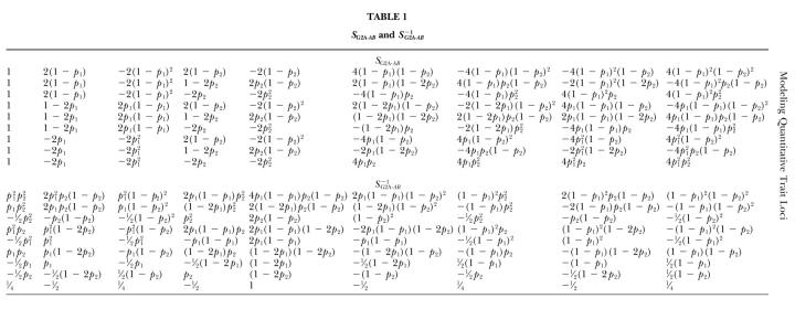
Details of S_G2A·AB and S⁻¹_G2A·AB are given in Table 1. They are simply the direct products of the matrices for loci A and B in (19) and (20) with some rearrangement of the columns and rows.

TABLE 1.

S_G2a·ab and s⁻¹_G2a·ab

In this model, a = p(G₂ − G₁) + (1 − p)(G₁ − G₀) for one locus, or a₁ = p₁(G_2· − G_1·) + (1 − p₁)(G_1· − G_0·) for two loci, where · denotes the mean, i.e., . Traditionally, a in this model is called the average effect, the allelic substitution effect averaged by allelic frequencies for different genotypes. The term average effect is used to distinguish it from a in the F_∞ or the F₂ model, which is usually called the additive effect, as this average effect is frequency dependent (Falconer and Mackay 1996). However, as emphasized throughout the article, the additive effect also depends on the model as a's in the F_∞, F₂, and UWR models are different in the context of multiple loci with epistasis.

What is the advantage of using the G2A model as compared to others, such as the F₂ or the F_∞ models for studying genetic effects and epistasis in a population where allelic frequencies are not one-half? Genetically, a major advantage is that the partition of genetic effects is directly related to the partition of the genetic variance. In an equilibrium population (in Hardy-Weinberg and linkage equilibrium), the additive effects contribute to the additive variance, the dominance effects contribute to the dominance variance, etc. There is no covariance between the genetic effects, due to the orthogonal property of the model.

This orthogonal property is also convenient for statistical tests and estimation of QTL effects, as the effects can be tested and estimated separately, although simultaneous estimation will always perform better statistically.

Hardy-Weinberg and linkage disequilibria do not change the definitions and also statistical estimation of the genetic effects with respect to the loci defined in a full model. In the above discussion for two loci with nine genotypic values and nine parameters, given a genetic-effect design matrix there is a unique solution for the parameter values in terms of the genotypic values. In the next section, we give a numerical example of three loci to show that the genetic effects for each model are the same for different configurations of allele frequencies and linkage disequilibrium in the full model, but not necessarily in a reduced model. In the appendix, we show this for the relatively simple case of a haploid model with two loci.

Disequilibrium will introduce genetic covariance between different effects. Since the genetic effects estimated in a disequilibrium population in the full model are the same as those in the equilibrium population for the loci concerned (if the loci are not in disequilibrium with other loci), the additive, dominance, and epistatic variances estimated in a disequilibrium population are still the same as those in the equilibrium population. But there are covariances between different genetic effects due to disequilibrium.

However, disequilibria will change the definition and estimation of genetic effects in a reduced model. For example, if two loci are in linkage disequilibrium, a separate estimation of the additive and dominance effects for each locus will include part of the effects of the other locus. By the same argument, if two loci are in Hardy-Weinberg and/or linkage disequilibria with other loci, the definition and statistical estimation of genetic effects for the two loci are affected by the disequilibria between the two loci and the other loci. If the other loci are identified, one way to reduce this influence is to fit all these loci simultaneously in a regression model for estimation, if feasible. So in a QTL analysis, when multiple loci are detected, it is always better to estimate the effects of multiple loci, including epistasis, together.

A NUMERICAL EXAMPLE

We use a numerical example to illustrate various points discussed and explore the properties and constraints of different models. We simulate three loci with the assumption that there is no three-locus epistasis but two-locus epistasis for pairs of loci. We discuss four different genotypic configurations with different allelic frequencies and linkage equilibrium or disequilibrium, assuming Hardy-Weinberg equilibrium. For three loci, the gametic frequencies can be expressed as

assuming no third-order linkage disequilibrium (D₁₂₃ = 0), where p_i, q_j, and r_k are allelic frequencies at loci 1, 2, and 3, and the D's are linkage disequilibria. The four cases are as follows:

• Case 1: p = ¹/₂ and D = 0 (Table 3). In this case, p₁ = q₁ = r₁ = 0.5 and D₁₂ = D₂₃ = D₁₃ = 0.

• Case 2: p = ¹/₂ and D ≠ 0 (Table 4). In this case, p₁ = q₁ = r₁ = 0.5, D₁₂ = D₂₃ = 0.125, and D₁₃ = 0.064.

• Case 3: p ≠ ¹/₂ and D = 0 (Table 5). In this case, p₁ = 0.7, q₁ = 0.6, r₁ = 0.3, and D₁₂ = D₂₃ = D₁₃ = 0.

• Case 4: p ≠ ¹/₂ and D ≠ 0 (Table 6). In this case, p₁ = 0.7, q₁ = 0.6, r₁ = 0.3, D₁₂ = D₂₃ = 0.112, and D₁₃ = 0.053.

TABLE 3.

Estimates of QTL effects by theF₂,F_∞, and UWR models forp = ¹/₂ andD = 0

									Loci 1 and 2				Loci 1 and 3				Loci 2 and 3
	σ2	μ	a1	d1	a2	d2	a3	d3	aa	ad	da	dd	aa	ad	da	dd	aa	ad	da	dd
F2	3.19	0.00	1.00	1.00
F∞	3.19	−0.50	1.00	1.00
UWR	3.19	−0.16	1.00	1.00
F2	2.44	0.00	1.00	1.00	1.00	1.00
F∞	2.44	−1.00	1.00	1.00	1.00	1.00
UWR	2.44	−0.33	1.00	1.00	1.00	1.00
F2	1.87	0.00	1.00	1.00	1.00	1.00			1.00	1.00	1.00	1.00
F∞	1.87	−0.75	0.50	0.50	0.50	0.50			1.00	1.00	1.00	1.00
UWR	1.87	−0.30	0.84	0.83	0.84	0.83			1.00	1.00	1.00	1.00
F2	1.69	0.00	1.00	1.00	1.00	1.00	1.00	1.00
F∞	1.69	−1.50	1.00	1.00	1.00	1.00	1.00	1.00
UWR	1.69	−0.50	1.00	1.00	1.00	1.00	1.00	1.00
F2	0.00	0.00	1.00	1.00	1.00	1.00	1.00	1.00	1.00	1.00	1.00	1.00	1.00	1.00	1.00	1.00	1.00	1.00	1.00	1.00
F∞	0.00	−0.75	0.00	0.00	0.00	0.00	0.00	0.00	1.00	1.00	1.00	1.00	1.00	1.00	1.00	1.00	1.00	1.00	1.00	1.00
UWR	0.00	−0.42	0.67	0.67	0.67	0.67	0.67	0.67	1.00	1.00	1.00	1.00	1.00	1.00	1.00	1.00	1.00	1.00	1.00	1.00

σ² is the unexplained residual genetic variance. The total genetic variance is 3.94.

TABLE 4.

Estimates of QTL effects by the F₂, F_∞, and UWR models forp = ¹/₂ andD ≠ 0

									Loci 1 and 2				Loci 1 and 3				Loci 2 and 3
	σ2	μ	a1	d1	a2	d2	a3	d3	aa	ad	da	dd	aa	ad	da	dd	aa	ad	da	dd
F2	3.14	0.77	1.03	0.45
	3.08	0.77			1.12	0.27
	3.15	0.77					1.03	0.45
	2.89	0.77	0.62	0.41	0.81	0.16
	2.79	0.77	0.82	0.42			0.82	0.42
	2.90	0.77			0.81	0.16	0.62	0.41
	2.71	0.77	0.62	0.40	0.50	0.06	0.62	0.40
F2	1.76	0.31	1.00	1.01	1.13	0.76			1.50	1.24	1.49	1.27
F∞	1.76	−0.25	0.38	0.37	0.38	0.12			1.50	1.24	1.49	1.27
UWR	1.76	0.05	0.79	0.80	0.88	0.55			1.50	1.24	1.49	1.27
F2	0.00	0.00	1.00	1.00	1.00	1.00	1.00	1.00	1.00	1.00	1.00	1.00	1.00	1.00	1.00	1.00	1.00	1.00	1.00	1.00
F∞	0.00	−0.75	0.00	0.00	0.00	0.00	0.00	0.00	1.00	1.00	1.00	1.00	1.00	1.00	1.00	1.00	1.00	1.00	1.00	1.00
UWR	0.00	−0.42	0.67	0.67	0.67	0.67	0.67	0.67	1.00	1.00	1.00	1.00	1.00	1.00	1.00	1.00	1.00	1.00	1.00	1.00

σ² is the unexplained residual genetic variance. The total genetic variance is 3.73.

TABLE 5.

Estimates of QTL effects by theF₂,F_∞, UWR, and G2A models forp ≠ ¹/₂ andD = 0

									Loci 1 and 2				Loci 1 and 3				Loci 2 and 3
	σ2	μ	a1	d1	a2	d2	a3	d3	aa	ad	da	dd	aa	ad	da	dd	aa	ad	da	dd
F2	3.67	−0.39	0.70	0.70
	3.45	−0.31			0.84	0.85
	1.58	0.56					1.50	1.51
G2A	3.67	−0.16	0.42	0.70
	3.45	−0.16			0.67	0.85
	1.58	−0.16					2.10	1.51
F2	1.04	0.19	0.69	0.68	0.84	0.85	1.50	1.50
G2A	1.04	−0.16	0.41	0.68	0.68	0.85	2.10	1.50
F2	3.12	−0.48	0.52	0.54	0.52	0.54			0.99	0.98	0.98	1.03
F∞	3.12	−0.76	0.03	0.02	0.03	0.02			0.99	0.98	0.98	1.03
UWR	3.12	−0.63	0.36	0.36	0.36	0.36			0.99	0.98	0.98	1.03
G2A	3.12	−0.16	0.42	0.71	0.67	0.85			0.48	0.57	0.78	1.03
F2	0.00	0.00	1.00	1.00	1.00	1.00	1.00	1.00	1.00	1.00	1.00	1.00	1.00	1.00	1.00	1.00	1.00	1.00	1.00	1.00
F∞	0.00	−0.75	0.00	0.00	0.00	0.00	0.00	0.00	1.00	1.00	1.00	1.00	1.00	1.00	1.00	1.00	1.00	1.00	1.00	1.00
UWR	0.00	−0.42	0.67	0.67	0.67	0.67	0.67	0.67	1.00	1.00	1.00	1.00	1.00	1.00	1.00	1.00	1.00	1.00	1.00	1.00
G2A	0.00	−0.16	0.42	0.70	0.67	0.84	2.10	1.50	0.48	0.60	0.80	1.00	0.84	0.60	1.40	1.00	1.12	0.80	1.40	1.00

σ² is the unexplained residual genetic variance. The total genetic variance is 3.83.

TABLE 6.

Estimates of QTL effects by the F₂, F_∞, UWR, and G2A models forp ≠ ¹/₂ andD ≠ 0

									Loci 1 and 2				Loci 1 and 3				Loci 2 and 3
	σ2	μ	a1	d1	a2	d2	a3	d3	aa	ad	da	dd	aa	ad	da	dd	aa	ad	da	dd
F2	3.88	0.34	0.04	−0.60
	3.62	0.24			0.80	−0.23
	1.12	1.23					1.75	1.60
G2A	3.88	0.40	0.28	−0.60
	3.62	0.40			0.85	−0.23
	1.12	0.40					2.39	1.60
F2	0.92	1.49	−0.46	−0.58	−0.35	−0.50	1.87	1.79
G2A	0.92	0.40	−0.23	−0.58	−0.25	−0.50	2.58	1.79
F2	2.93	−0.21	0.38	0.38	0.62	−0.08			1.70	1.22	1.69	1.24
F∞	2.93	−0.05	−0.23	−0.24	−0.23	−0.70			1.70	1.22	1.69	1.24
UWR	2.93	−0.23	0.18	0.18	0.34	−0.29			1.70	1.22	1.69	1.24
G2A	2.93	0.14	0.42	0.70	1.10	0.31			0.88	0.73	1.44	1.24
F2	0.00	0.00	1.00	1.00	1.00	1.00	1.00	1.00	1.00	1.00	1.00	1.00	1.00	1.00	1.00	1.00	1.00	1.00	1.00	1.00
F∞	0.00	−0.75	0.00	0.00	0.00	0.00	0.00	0.00	1.00	1.00	1.00	1.00	1.00	1.00	1.00	1.00	1.00	1.00	1.00	1.00
UWR	0.00	−0.42	0.67	0.67	0.67	0.67	0.67	0.67	1.00	1.00	1.00	1.00	1.00	1.00	1.00	1.00	1.00	1.00	1.00	1.00
G2A	0.00	−0.16	0.42	0.70	0.67	0.84	2.10	1.50	0.48	0.60	0.80	1.00	0.84	0.60	1.40	1.00	1.12	0.80	1.40	1.00

σ² is the unexplained residual genetic variance. The total genetic variance is 3.98.

The genotypic values are presented in Table 2 and follow an F₂ model with all additive, dominance, and pairwise epistatic effects being one and no three-locus epistasis. This configuration of genotypic values is given in Table 2. To minimize sampling effects, we simulate 100,000 individuals following the genotypic frequency configuration for each case. The genotypic values are regressed to genetic-effect design variables of different models for one, two, or three loci. No environmental variance is considered. Results of parameter estimation and residual genetic variance for each analysis are given in Tables 3–6.

TABLE 2.

Genotypic values used for the numerical example

	AA			Aa			aa
	CC	Cc	cc	CC	Cc	cc	CC	Cc	cc
BB	2.25	2.25	−1.75	2.25	2.25	−1.75	−1.75	−1.75	−1.75
Bb	2.25	2.25	−1.75	2.25	2.25	−1.75	−1.75	−1.75	−1.75
bb	−1.75	−1.75	−1.75	−1.75	−1.75	−1.75	−1.75	−1.75	2.25

Table 3 shows the comparison of the F₂, F_∞, and UWR models for the case p = ¹/₂ and D = 0. As expected, estimates of the additive and dominance effects are the same for the three models if the epistatic effects are not fitted in the regression; otherwise they are different. Since genotypic frequencies follow from the F₂ ratio, estimates of the additive and dominance effects under the F₂ model are independent of the estimation of the epistatic effects, showing the orthogonal property. However, estimates of the additive and dominance effects under the F_∞ and UWR models are different when the epistatic effects are also estimated.

Also all three models give the same estimates of epistatic effects as expected. However, in this case, we did not simulate three-locus epistasis; otherwise estimates of the pairwise epistatic effects would be different if the three-locus epistatic effect is fitted for the F_∞ and UWR models, but not for the F₂ model. No matter which model is used, the genetic variance explained is the same for the same analysis. Different models just provide different ways to partition the genetic effects with the same variance, and the orthogonal model does provide a convenient way to estimate and interpret different genetic effects. Note in this case it just happens that when all effects of three loci are fitted, the F_∞ model gives zero additive and dominance effects and may suggest no main effects, only epistatic effects. So, modeling does matter when it comes to genetic interpretation.

Table 4 shows the comparison for the case p = ¹/₂ and D ≠ 0. Since the three models give the same estimates of main effects when epistatic effects are not fitted, only the F₂ estimates are given. As the loci are in linkage disequilibrium, estimates of the genetic effects (main and epistatic effects) in reduced models are biased by linkage disequilibrium, and the separate and joint estimations are different. However, they are unbiased in the full model, a point discussed above and also in the appendix. This is also shown in Tables 5 and 6.

For unequal allelic frequencies (the case p ≠ ¹/₂ and D = 0), we compare the G2A model with the other models in Table 5. In this case, the G2A model shows that the estimation of the additive and dominance effects is independent of epistatic effects. The small difference in different estimates for the G2A model is due to sampling.

With both unequal allelic frequencies and linkage disequilibrium (the case p ≠ ¹/₂ and D ≠ 0) in Table 6, the estimation of genetic effects and the interpretation of estimates are quite complicated. The estimates in the full and reduced models are all different. In this example, some estimates in the reduced models are even negative. Although in the full model the estimation of genetic effects specified by a model is consistent and independent of the genotypic frequency configuration as long as all relevant genotypes are observed, in realty the so-called full model is unknown and can be very complex. Any practical estimation would be almost always in a reduced model and could be influenced by disequilibrium and epistasis between detected and undetected loci.

DISCUSSION

In this article, we compare several models for analyzing QTL effects and epistasis. The difference among the F₂, F_∞, and UWR models is in the definition of the dominance-effect design variable, which reflects the difference of the mean (departure point) for a model. This difference does not affect the definition of additive and dominance effects at one locus, but does at multiple loci with epistasis. The same argument also applies to the definition of pairwise epistatic effects if higher-order epistasis is considered, which is not specifically analyzed in this article. This has implications for QTL analysis. One implication is that estimates of additive and dominance effects are not consistent for the F_∞ model as well as for the UWR model in a mapping population such as an F₂ population, as the estimates depend on whether epistatic effects are fitted in the model. This could cause unnecessary complications in interpreting the genetic basis and architecture of quantitative trait variation in a mapping population.

When modeling QTL, the consistency of model parameters in a multilocus setting is an important consideration. It is important for a model to be multilocus comparable and consistent, so that the relationships within and between loci can be clearly and readily analyzed, estimated, and interpreted. Here the consistency means that the effect of a QTL is consistently defined in a reference equilibrium population for one, two, or more loci. In statistics, this is called orthogonality. This property is particularly important for the study of epistasis. Orthogonality ensures that the additive, dominance, and epistatic effects can be independently estimated for one, two, three, or more loci in the reference population where the model is defined and interpreted. Thus, if the number of QTL is incorrectly identified, which seems to be always the case in practice, the parameter values for those identified QTL can still be consistently estimated.

Disequilibrium complicates matters. Linkage disequilibrium would complicate the definition of genetic effects, the partition of genetic variance, and could certainly bias the estimation of parameter values for those identified QTL if the QTL model (number and genomic position of QTL) is inferred incorrectly. It could also complicate the detection of QTL and epistasis, i.e., model identification. If multiple QTL are detected, it is always preferable to have different QTL effects, including epistatic effects, estimated together if possible. This joint estimation of additive, dominance, and epistatic effects is also consistent with the partition of genetic variance in the mapping population and is very convenient for the interpretation of the estimated genetic variances and covariances explained by QTL effects. The variances of QTL effects would correspond to those partitions in an equilibrium population, and covariances between QTL effects reflect the level of disequilibrium in the estimation population. This is the approach of multiple-interval mapping (Kao et al. 1999; Zeng et al. 1999) that estimates the genetic effects, including epistatic effects, and partitions the genetic variances for multiple loci simultaneously in QTL analysis.

With a finite sample size in many QTL mapping experiments, there is a practical problem in estimating the genetic effects, including epistatic effects, in a “full model” as some genotypes involving two or more loci may be observed rarely or not at all. In multiple-interval mapping, one way to deal with this problem is to select a subset of statistically significant genetic effects, including epistatic effects, for simultaneous estimation, given the identification of multiple QTL or multiple genomic positions.

Another point is that different models can interpret some important genetic quantities differently. For example, heterosis is measured as the difference between the F₁ and the mean of parental lines on some quantitative traits. If the parental lines are inbred and designated as G₂₂ and G₀₀ for a two-locus model, heterosis is measured as G₁₁ − (G₂₂ + G₀₀)/2, where G₁₁ is the genotypic value of the F₁. However, for the F_∞ model

and for the F₂ model

If we generalize it to multiple loci and ignore epistasis involving three or more loci, we obtain

In this case, the dominance effects in the two models are defined differently. For the numerical example of three loci in Table 2, there is no heterosis as G₁₁₁ − (G₂₂₂ + G₀₀₀)/2 = 2.25 − (2.25 + 2.25)/2 = 0. However, the genetic interpretation is different for the two models. For the F_∞ model, this is to due to canceling out between the additive × additive effects and the dominance × dominance effects, as (aa)₁₂ = (aa)₁₃ = (aa)₂₃ = 1, (dd)₁₂ = (dd)₁₃ = (dd)₂₃ = 1, and d₁ = d₂ = d₃ = 0 (Table 3). For the F₂ model, this is due to canceling out between the dominance effects and the additive × additive effects, as (aa)₁₂ = (aa)₁₃ = (aa)₂₃ = 1, (dd)₁₂ = (dd)₁₃ = (dd)₂₃ = 1, and d₁ = d₂ = d₃ = 1 (Table 3). The epistasis involving three loci is assumed to be absent in the numerical example.

One caution in using the F_∞ model to estimate the genetic effects and interpret heterosis is that the dominance effects under the F_∞ model should be estimated together with the epistatic effects. Otherwise, the genetic interpretation of heterosis is different. If the dominance effects are estimated for each locus separately, which would be equivalent to those under the F₂ model for unlinked loci, the dominance × dominance effects should not be counted as a part of heterosis.

Different investigators may prefer different models. Model parameters are transferable between different models (Van Der Veen 1959). However, it would make much better sense to use an orthogonal model for QTL analysis in a segregating population for the consistency in estimating genetic effects and partitioning genetic variance components.

APPENDIX

We demonstrate that the partial regression coefficients in a disequilibrium population are equal to the simple regression coefficients in an equilibrium population in the full model for a relatively simple case of a two-locus haploid model. For comparison, we also present the composition of the additive effects in a reduced model without an epistatic effect.

Consider a locus with alleles A and a having frequencies p₁ and 1 − p₁, respectively. Define an indicator variable

We can express the haploid model as

with

A1

If we extend the model to two loci and define indicator variables z₂ and x₂ for locus B accordingly, we have

including the epistatic effect aa. Using the direct product, we obtain

A2

and

A3

With four genotypes and four parameters, there is a unique relationship between the parameters and genotypic values. This relationship will not depend on the genetic structure of the population. Whether the model is applied to an equilibrium or disequilibrium population, the genetic effects will be the same.

Nevertheless, in the following, we show this conclusion in a different way. The genetic effects a₁, a₂, and aa are partial regression coefficients in the regression model. If loci are in linkage equilibrium, x₁ and x₂ are independent, i.e., E(x₁x₂) = E(x₁)E(x₂) = 0, and the partial regression coefficients are equal to the simple regression coefficients:

Note that E(z_i) = Ez²_i = p_i and E(x_i) = 0 for i = 1, 2. These variances and covariances are

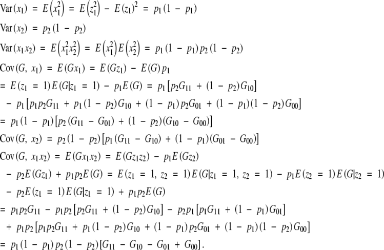Then for an equilibrium population, we have shown

A4

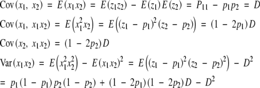
To consider a disequilibrium population, we note that the genotypic frequencies are P₁₁ = p₁p₂ + D, P₁₀ = p₁(1 − p₂) − D, P₀₁ = (1 − p₁)p₂ − D, and P₀₀ = (1 − p₁)(1 − p₂) + D, where D is a measure of linkage disequilibrium. The partial regression coefficients are

A5

with

and

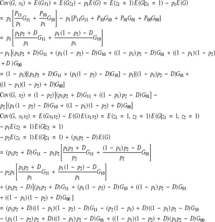Inserting these variances and covariances in (A5), inverting the matrix and multiplying it by the covariance vector, one obtains

A6

Equation (A6) is the same as (A3) and (A4) with regard to the definition of a₁, a₂, and aa. This shows that the partial regression coefficients in a disequilibrium population are equal to the simple regression coefficients in the equilibrium population in this full model with two loci and correspond to the initial model specification.

However, if we fit only the additive effects without the epistatic effect in the following regression model,

the partial regression coefficients of a₁ and a₂ would be

In this case,

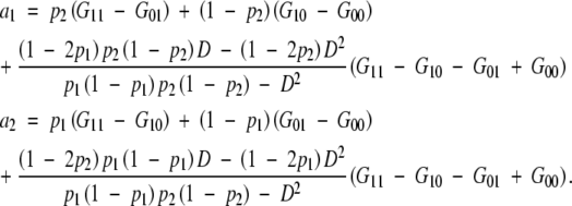These are equal to the additive effects in the full model if D = 0, G₁₁ − G₁₀ − G₀₁ + G₀₀ = 0 (no epistasis), or p₁ = p₂ = ¹/₂.

References

- Anderson, V. L., and O. Kempthorne, 1954. A model for the study of quantitative inheritance. Genetics 39 883–898. [DOI] [PMC free article] [PubMed] [Google Scholar]
- Cheverud, J. M., 2000 Detecting epistasis among quantitative trait loci, pp. 58–81 in Epistasis and the Evolutionary Process, edited by J. B. Wolf, E. D. Brodie III and M. J. Wade. Oxford University Press, Oxford.
- Cheverud, J. M., and E. J. Routman, 1995. Epistasis and its contribution to genetic variance components. Genetics 139 1455–1461. [DOI] [PMC free article] [PubMed] [Google Scholar]
- Cockerham, C. C., 1954. An extension of the concept of partitioning hereditary variance for analysis of covariances among relatives when epistasis is present. Genetics 39 859–882. [DOI] [PMC free article] [PubMed] [Google Scholar]
- Cockerham, C. C., and Z-B. Zeng, 1996. Design III with marker loci. Genetics 143 1437–1456. [DOI] [PMC free article] [PubMed] [Google Scholar]
- Eberhart, S. A., and C. O. Gardner, 1966. A general model for genetic effects. Biometrics 22 864–881. [Google Scholar]
- Falconer, D. S., and T. F. C. Mackay, 1996 Introduction to Quantitative Genetics, Ed. 4. Longman, Harlow, UK.
- Fisher, R. A., 1918. The correlation between relatives on the supposition of Mendelian inheritance. Trans. Roy. Soc. Edinburgh 52 399–433. [Google Scholar]
- Griffing, B., 1956. Concept of general and specific combining ability in relation to diallel crossing systems. Aust. J. Biol. Sci. 9 463–493. [Google Scholar]
- Hayman, B. I., 1957. Interaction, heterosis and diallel crosses. Genetics 42 336–355. [DOI] [PMC free article] [PubMed] [Google Scholar]
- Hayman, B. I., and K. Mather, 1955. The description of genetic interactions in continuous variation. Biometrics 11 69–82. [Google Scholar]
- Hill, W. G., 1982. Dominance and epistasis as components of heterosis. Z. Tierz. Zuchtungsbio. 99 161–168. [Google Scholar]
- Kao, C.-H., and Z-B. Zeng, 2002. Modeling epistasis of quantitative trait loci using Cockerham's model. Genetics 160 1243–1261. [DOI] [PMC free article] [PubMed] [Google Scholar]
- Kao, C.-H., Z-B. Zeng and R. D. Teasdale, 1999. Multiple interval mapping for quantitative trait loci. Genetics 152 1203–1216. [DOI] [PMC free article] [PubMed] [Google Scholar]
- Mather, K., and J. L. Jinks, 1982 Biometrical Genetics, Ed. 3. Chapman & Hall, London.
- Routman, E. J., and J. M. Cheverud, 1997. Gene effects on a quantitative trait: two-locus epistatic effects measured at microsatellite markers and at estimated QTL. Evolution 51 1654–1662. [DOI] [PubMed] [Google Scholar]
- Van Der Veen, J. H., 1959. Tests of non-allelic interaction and linkage for quantitative characters in generations derived from two diploid pure lines. Genetica 30 201–232. [DOI] [PubMed] [Google Scholar]
- Zeng, Z-B., C.-H. Kao and C. J. Basten, 1999. Estimating the genetic architecture of quantitative traits. Genet. Res. 74 279–289. [DOI] [PubMed] [Google Scholar]