Stochastic Models for Horizontal Gene Transfer

Abstract

Horizontal gene transfer (HGT) plays a critical role in evolution across all domains of life with important biological and medical implications. I propose a simple class of stochastic models to examine HGT using multiple orthologous gene alignments. The models function in a hierarchical phylogenetic framework. The top level of the hierarchy is based on a random walk process in “tree space” that allows for the development of a joint probabilistic distribution over multiple gene trees and an unknown, but estimable species tree. I consider two general forms of random walks. The first form is derived from the subtree prune and regraft (SPR) operator that mirrors the observed effects that HGT has on inferred trees. The second form is based on walks over complete graphs and offers numerically tractable solutions for an increasing number of taxa. The bottom level of the hierarchy utilizes standard phylogenetic models to reconstruct gene trees given multiple gene alignments conditional on the random walk process. I develop a well-mixing Markov chain Monte Carlo algorithm to fit the models in a Bayesian framework. I demonstrate the flexibility of these stochastic models to test competing ideas about HGT by examining the complexity hypothesis. Using 144 orthologous gene alignments from six prokaryotes previously collected and analyzed, Bayesian model selection finds support for (1) the SPR model over the alternative form, (2) the 16S rRNA reconstruction as the most likely species tree, and (3) increased HGT of operational genes compared to informational genes.

TRADITIONAL views of molecular evolution hold that genetic material mutates slowly over time as it is passed in a vertical fashion from parent to progeny. Molecular phylogenetics then aims to reconstruct this history of inheritance of genetic sequence data from contemporary organisms into a tree-like structure. However, belief in a single tree, mandated by vertical transmission, for all genetic material is changing. Evolutionary biologists increasingly recognize the horizontal transmission of genetic material between distantly related organisms as an important mechanism of evolution (Syvanen 1994; Lawrence 1999; Jain et al. 2002).

The process of horizontal (or lateral) gene transfer (HGT) plays a critical role across all domains of life and in particular among prokaryotes (Jain et al. 1999; Koonin et al. 2001). For example, many prokaryotes are agile at quickly adapting to new environments. Often, this ability stems from the acquisition of new genes through HGT rather than through random mutation (Lawrence 1999). At least three mechanisms promote HGT in prokaryotes (Jain et al. 2002). These include: (1) transformation in which free DNA sequences are absorbed from the environment, (2) conjugation between two different prokaryotic species, and (3) transduction of genetic material through viruses. Finally, HGT also has medical importance (Brown 2003). In the field of infectious diseases, HGT among bacterial pathogens of antibiotic resistance genes has greatly contributed to the emergence of multidrug-resistant bacteria in clinical settings (Leverstein-van Hall et al. 2002). In the field of oncology, HGT may also affect tumor progression; Bergsmedh et al. (2001) show that eukaryotic cells can transfer active oncogenes.

Three general methods have been employed to examine HGT. The first focuses on single genomes and identifies genes suspected to have been imported through HGT by examining variation in nucleotide base composition and codon usage patterns (Lawrence and Ochman, 1997). The latter two methods are comparative studies across species. One uses similarity approaches based on gene content to identify HGT (Ragan 2001) and to propose average genome or species-level trees (Snel et al. 1999), while the alternative method endorses phylogenetic reconstruction using orthologous genes (Jain et al. 1999). Base composition and codon bias studies may perform poorly when compared to phylogenetic methods (Koski et al. 2001). Further, phylogenetic methods offer at least one advantage over similarity-based approaches. The reconstructed phylogenies have direct biological interpretability as descriptions of the underlying evolutionary histories of the different genes (Doolittle 1999). If a reconstructed gene tree differs from the assumed phylogeny of the species being studied, then HGT is offered as a possible explanation (Syvanen 1994). One intrinsic difficulty is that the true species tree is often itself unknown. Therefore, it is necessary to either fix the species tree to equal the inferred gene tree for a specially chosen gene, e.g., the 16S rRNA tree (Woese 2000), or simultaneously estimate the species tree and gene trees given a biologically plausible model relating them. As a first step, several research groups have attacked the inverse problem of reconstructing a species tree given gene trees subject to HGT. Most notable are the parsimony-based reconciled tree work by Page and colleagues (e.g., Page 2000) and the algorithmic work of Mirkin et al. (2003).

I propose a simple class of stochastic models for HGT that enable the simultaneous estimation of the underlying species tree relating a group of organisms and the gene trees subject to HGT for a set of orthologous gene alignments. These HGT models function in a hierarchical manner (Suchard et al. 2003a) in which standard Bayesian phylogenetic approaches (e.g., Sinsheimer et al. 1996; Yang and Rannala 1997; Mau et al. 1999; Li et al. 2000; Huelsenbeck et al. 2001) are used to reconstruct each gene tree from its corresponding gene alignment. Simultaneous to the reconstructions, the HGT models impose a second probabilistic distribution over the gene trees (Maddison 1997). This hierarchical distribution describes the gene trees likelihoods given an unknown species tree and an unknown number of HGT events leading from that species tree to each gene tree. The model is fit in a Bayesian framework that naturally handles uncertainty in discrete parameters such as all the trees and the number of HGT events and compares various models using Bayes factors (Suchard et al. 2001). Stochastic models fit in statistical frameworks offer several advantages over parsimony approaches. First, parsimony may underestimate the number of HGT events linking the species tree to the gene trees. This consequence is similarly seen in parsimonious reconstructions of the tree themselves, in which the number of nucleotide substitutions is underestimated. Second, it is easier in a statistical framework to include measures of uncertainty and these levels may be high in the inferred gene trees given the sparse data from which they are reconstructed.

One additional advantage of building stochastic models for HGT is the ability to compare competing models and to incorporate possible differences in the stochastic processes across genes, while assessing the significance of these differences in a formal statistical framework. As one example of possible differences across genes, Jain et al. (1999) propose the complexity hypothesis. Under this hypothesis, genes are divided into one of two classes, informational or operational genes. Between classes, the rates of HGT differ. It is suspected that rates are higher for operational genes than for informational genes. This hypothesis and others can be tested by integrating over all possible species trees and gene trees weighed by their posterior probabilities. This Bayesian model-averaging approach reduces the possible bias inherent in selecting a specific species tree, minimizes underestimation of the uncertainty associated with the hypotheses (Taylor et al. 1996), and eliminates the need for ad hoc analyses. Formal comparison of different models for HGT will help gather further insight into the underlying biological processes.

MODEL

Within-gene reconstruction model:

I begin with a hierarchical framework for phylogenetic reconstruction using molecular sequence data Y (Suchard et al. 2003a). Data Y = (Y₁, … , Y_K) consist of K naturally disjoint partitions. Partition data Y_k for k = 1, … , K represent the aligned DNA sequences of length L_k from one specific gene per partition, sequenced from the same N taxa across all partitions. A hierarchical phylogenetic model enables the pooling of information across gene partitions to improve estimate precision in individual partitions, while permitting estimation and testing of tendencies in across-partition quantities. For HGT, such across-partition quantities include: (1) an overall species tree, (2) appropriate stochastic models from which to construct a probability distribution over individual gene trees given the species tree, and (3) the stochastic model parameters that may vary between different classes of genes.

To utilize standard Bayesian models for phylogenetic reconstruction (e.g., Sinsheimer et al. 1996; Yang and Rannala 1997; Mau et al. 1999; Li et al. 2000) within a gene partition, data Y_k further divide into ordered homologous sites Y_kl for l = 1, … , L_k. Site data Y_kl = (Y_kl1, … , Y_klN)^t contain one nucleotide from each taxon, such that Y_kln ∈ (A, G, C, T) or their ambiguous wildcards for n = 1, … , N. I assume that sites within a partition are independent and identically distributed, and the likelihood of observing Y_kl is given by a multinomial distribution over the 4^N possible outcomes with ambiguous nucleotides being integrated over their possible realizations. The multinomial outcome probabilities become functions of an unknown tree τ_k that describes the relatedness of the N taxa, branch lengths t_k = (t_k1, … , t_kB), and a model to describe nucleotide mutation along these branches, all within partition k.

I elect for a reversible, continuous-time Markov chain (CTMC) model for nucleotide substitution (Felsenstein 1981) popularized by Tamura and Nei (1993) (TN93). The TN93 model is further parameterized by two transition:transversion rate ratios, α_k between purines A and G and γ_k between pyrimidines C and T, and the stationary distribution of the underlying Markov chain π_k = (π_kA, π_kG, π_kC, π_kT). The final scale parameter in the TN93 model is fixed such that branch lengths measure the expected number of nucleotide substitutions between the nodes in τ_k that the branch connects. Because I assume a reversible model for nucleotide substitution and make no clock-like restrictions on branch lengths, the root of each tree is unidentifiable (Felsenstein 1981). As a consequence, the descriptions of all trees to follow are unrooted with N − 2 internal nodes and B = 2N − 3 branches.

Across-gene hierarchical model:

Following the hierarchical framework of Suchard et al. (2003a), I take branch lengths t_k as exponentially distributed with unknown expected divergence μ_k within partition k and model

and

1

where V = (A, G, M)^t and Π = (Π_A, Π_G, Π_C, Π_T) are unknown across-partition-level expectations, variance-covariance matrix has diagonal form, and σ⁻²_α, σ⁻²_γ, σ⁻²_μ, and N_Π are unknown across-partition-level measures of precision. Leaving V, Σ, Π, and N_Π as unknowns specified only by hyperprior distributions and estimating these parameters simultaneously with the within-partition-level continuous parameters, α_k, γ_k, and μ_k for all k, enables the borrowing of strength of information from one partition by another, producing more precise within-partition-level estimates. I assume conjugate (when possible) and flat or noninformative hyperpriors on these across-partition-level parameters, as discussed in Suchard et al. (2003a). While the development of hierarchical priors over the continuous within-partition-level parameters has been straightforward, constructing a hierarchical prior over gene trees τ_k that incorporates the stochastic nature of HGT is more involved. This is illustrated in the next section.

Horizontal gene transfer models:

To build a stochastic model for HGT, I first present a formal description of the set of all possible N-taxon trees, commonly referred to as “tree space” (Billera et al. 2001), as a mathematical graph and then discuss several possible random walks (D. Aldous and J. Fill, unpublished results) on this graph that mirror the observed effects of HGT.

There exist M = (2N − 5)!/2^N−3(N − 3)! possible trees relating N extant taxa (Felsenstein 1981). On the basis of these M trees, I construct a graph 𝒢 = (ν, ε) with vertex set ν and edge set ε. Each tree represents a different vertex, or node, in the graph, such that the size of the vertex set |ν| = M. An edge uv ∈ ε of a graph describes a direct connection between two of the graph's vertices u, v ∈ ν. The number of edges emanating from a single vertex v defines its degree d(v). Two vertices that are joined together by a single edge are called adjacent. Restricting attention to simple graphs in which pairs of vertices may be connected to each other only by a single edge and no vertex is connected to itself by a looping edge, a single vertex v from graph 𝒢 may be adjacent from as few as zero to as many as M − 1 other vertices. The set of all vertices adjacent to v are its neighborhood Γ(v) and the size of this neighborhood |Γ(v)| = d(v). The specification of a neighborhood for each vertex completes the description of 𝒢, and many choices are available.

Subtree-prune-regraft-based model:

One approach to defining neighborhoods for each possible tree stems from subtree transfer operations (Allen and Steel 2001). Subtree transfer operators act on trees producing local rearrangements. Applying a subtree transfer operator to one tree τ results in the creation of one of several possible new topologies that differs from τ by an extent dependent on the operator. The collection of all trees one operation away from τ = v becomes its neighborhood Γ(v) under that operator. Nearest-neighbor interchange (Robinson 1971), tree bisection and reconnection (Swofford et al. 1996), and subtree prune and regraft (SPR) (Hein 1990, 1993) are three examples. In light of the goals of this article, SPR offers an advantage over the former two operators because of its potential biological interpretation. Applying the SPR operator to τ = v with its resultant drawn from Γ_SPR(v) mirrors the differences observed between a species tree and an individual gene tree affected by one HGT (or recombination) event (Hein 1990, 1993; Jain et al. 1999; Allen and Steel 2001).

Figure 1 illustrates one realization of the SPR operator applied to a six-taxon tree. The operator works in two steps. The first step selects and cuts any branch in the initial tree, τ_initial. Cutting the branch prunes away a subtree, τ_subtree. This subtree then regrafts itself using the same cut branch to a new internal node obtained by subdividing a preexisting branch in τ_initial − τ_subtree.

Figure 1.—

Subtree prune and regraft operator applied to a six-taxon tree. (1) Operator selects and cuts any branch in the initial tree, pruning away a subtree. (2) Operator regrafts subtree by selecting and subdividing a preexisting branch in the remaining tree. (3) Resultant tree for this realization.

Several important properties about the graph 𝒢_SPR induced by the SPR operator have been previously studied. First, 𝒢_SPR is regular, implying that every vertex v ∈ ν_SPR possesses the same degree d(v) = 2(N − 3)(2N − 7) and, hence, neighborhood size (Allen and Steel 2001). Also, 𝒢_SPR is connected, meaning that a sequence of consecutive edges (a path) exists, connecting every pair of vertices in 𝒢_SPR (Robinson 1971; Allen and Steel 2001).

One straightforward stochastic process on any simple graph 𝒢 is an unweighted random walk. A random walk on 𝒢 proceeds from vertex to vertex along existing edges of the graph, generating a discrete-time Markov chain (DTMC), where the states of the chain are the visited vertices. As unweighted, the chain uniform randomly chooses its next vertex to visit from all neighbors of its current vertex. For this DTMC, the one-event transition probability matrix A has entries

2

defining the probability of u changing into v as a result of one random event. It should be noted that A is just the adjacency matrix of 𝒢 rescaled to be a stochastic matrix [i.e., ∑_v(A)_uv = 1].

On the basis of K random walks on the graph 𝒢_SPR induced by the SPR operator, I construct a hierarchical prior over the joint distribution of all gene trees τ_k. To accomplish this task, I assume:

• An unknown species tree Υ exists.

• The vertex representing Υ is the initial state of K Markov chains.

• The Markov chains are conditionally independent given Υ and A.

• The vertex representing τ_k is the final state of the kth chain.

• And each chain is of unknown length 0 ≤ E_k < ∞.

Figure 2 depicts one set of the possible paths of K = 4 Markov chains starting at species tree Υ and ending at gene trees τ_k on a small portion of a representative graph. The lengths of paths E_k shown range from one to three. I illustrate no paths of length zero, but these realizations should be most likely. A parsimony-like analysis considering beginning and end points of the chains in Figure 2 would, for example, underestimate E₄ as zero instead of three.

Figure 2.—

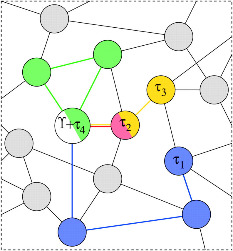
One possible Markov chain realization on a simplified graph for the species tree Υ and four gene trees τ₁, … , τ₄. All chains begin at the same vertex representing the species tree Υ (in white). The chain producing gene tree τ₁ has length E₁ = 3 (blue), the chain for τ₂ has length E₂ = 1 (red), the chain for τ₃ has length E₃ = 2 (yellow), and the chain for τ₄ has length E₄ = 3 (green). Note that this latter chain returns to its starting state; a parsimony-like analysis would estimate E₄ = 0. Not depicted are chains with actual length zero; these are most probable a priori.

Given the assumptions listed above, the probability of species tree Υ giving rise to gene tree τ_k after E_k HGT events is

3

To complete the hierarchical specification, I assign a prior distribution over Υ by letting

4

where z = (z₁, … , z_M) are constants, the prior probabilities of the M possible N-taxon trees. When little or no information is available about Υ, one reasonable choice is z₁ = … = z_M = 1/M; alternately, one may choose z such that the prior odds of competing hypotheses regarding Υ are one in a hypothesis-testing setting (Suchard et al. 2003a). A further choice is discussed later. I further assume a conditionally independent prior on all E_k,

5

where Λ_k is the expected number of HGT events for gene k and is a deterministic function of across-gene-level parameters. This prior is conjugate to (3), allowing all E_k to be integrated out of the model, improving sampling efficiency (Liu 1994),

6

Letting q(τ_k = v|Υ = u, Λ_k) = (P)_uv, the multistep transition probability matrix,

7

where I is the M × M identity matrix and Q = P − I is the CTMC infinitesimal rate matrix representation of the HGT process. In this parameterization, Λ_k are scaled as the expected number of HGT events per gene. Let Λ = (Λ₁, … , Λ_K). Then, recalling the conditional independence assumption between Markov chains, the joint distribution over all gene trees τ_k becomes

8

Calculating the probabilities in (8) requires numerical methods to determine the matrix exponential involving P_SPR. These methods involve calculating the complete set of eigenvalues and eigenvectors of P_SPR, requiring 𝒪(M³) operations. Such procedures become quickly computationally prohibitive as N, and hence M, increases. As a consequence, numerical approximations may be necessary to develop weighted graph extensions to 𝒢_SPR directly. The weights in these extended graphs would be functions of unknown parameters and sampling these parameters would necessitate repetitive diagonalization.

Random walks with analytic solutions:

An alternative to this computational barrier involves using random walks on graphs for which analytic solutions are known for any size M. To help find such solutions, Equation 7 demonstrates the close connection between a DTMC with a Poisson-distributed number of events and a CTMC. In fact, any such DTMC can be expressed as a unique CTMC, called the “continuized” version (D. Aldous and J. Fill, unpublished results). Analytic solutions for several weighted and unweighted CTMC processes on a complete graph are commonly used in phylogenetics. In a complete graph, all vertices are adjacent to all others. The most notable examples are the CTMC models for nucleotide substitution. The simplest model by Jukes and Cantor (1969) is unweighted. In the appendix, I present the multistep transition probability matrix P_GJC for a generalized Jukes-Cantor (GJC) model involving an arbitrary number of vertices M. Proposed by Kimura (1980), the next most sophisticated model for a complete graph is weighted. This model presupposes that the vertices are divided into two disjoint sets, ν₁ ∪ ν₂ = ν, and that transitions within and between ν₁ and ν₂ occur at varying rates. In terms of HGT, such a weighted random walk may prove useful to model varying rates of HGT between different groups of taxa. Letting M₁ = |ν₁|, M₂ = |ν₂|, and R equal the ratio of within- to between-transition rates, I present the multistep transition probability matrix P_GK given M₁, M₂, and R for a generalized Kimura (GK) model in the appendix.

Modeling differences across gene classes:

I incorporate potential differences across genes in the expected number of HGT events Λ_k by employing a generalized linear model (GLM) approach (McCullagh and Nelder 1983). GLMs link the mean response, in this case Λ_k, to a set of linear predictors. First, I divide all K genes into one of C possible classes, where the definition of the classes depends on the specific research question at hand. To identify gene-class membership in the GLM, I construct a K × C design matrix D = (D_kc), where matrix elements D_k1 = 1 for all k, representing the baseline multiplier for the reference class, and

9

for c = 2, … , C, representing the offset multipliers for the remaining classes. Such a design matrix is standard in regression problems involving categorical dependent variables. I model

10

where linear combinations of predictors λ = (λ₁, … , λ_C) specify, on the log-scale, the expected number of HGT events for all classes. I complete the hierarchical prior specification by assuming

11

I set L = (−2, 0, … , 0) and Ψ = diag(10, … , 10). This provides a quite diffuse prior on λ, with the median expected number of HGT events per gene ≈ 0.14 (Garcia-Vallve et al. 2000) for all classes.

As an example of how this GLM construction functions, consider the C = 2 classes case. Then,

12

When λ₂ = 0, no difference across classes exists. Likewise, when λ₂ < 0, the expected number of HGT events per gene is smaller in class 2 than in class 1, and when λ₂ > 0, the expected number is larger.

STATISTICAL FRAMEWORK

Comparing the relative appropriateness of the various stochastic models for HGT proposed in preceding sections and testing for significant differences in the expected number of HGT events across genes can be accomplished using Bayesian model selection via Bayes factors. Bayes factors are the Bayesian analog of the likelihood-ratio test (LRT), but suffer from fewer difficulties than LRTs in discrete spaces, when comparing non-nested models and with sparse data (Suchard et al. 2001). A Bayes factor B₁₀ measures the relative change in the support of the data Y in favor of one statistical model M₁ over another model M₀ and equals the ratio of the marginal likelihood m(Y|M₁) of M₁ over the marginal likelihood m(Y|M₀) of M₀ (Kass and Raftery 1995). To calculate Bayes factors, frequently more efficient methods than estimating the multidimensional integrals hidden in the marginal likelihoods directly are available.

When models are nested, a relatively simple Bayes factor calculation is available via the Savage-Dickey ratio (Verdinelli and Wasserman 1995) and involves generating a posterior sample from the larger model only (Suchard et al. 2003b). For example, to assess the significance of differences across gene classes in the expected number of HGT events, let M₁ represent the unrestricted model proposed above. Nested within M₁ exists M₀, the equal-rates model, where λ_c = 0 for c = 2, … , C. Further, the GJC model is nested within the GK model, as both are equal when R = 1.

On the other hand, the GJC and SPR models are non-nested, but both possess zero free parameters in their respective P matrices. For two arbitrary models M₀ and M₁ in situations like this, it is possible to estimate the posterior probabilities p(M₀|Y) and p(M₁|Y) by constructing a mixture model over the joint space of M₀ and M₁. By applying the Bayes theorem,

13

where q(M₀) and q(M₁) are the prior probabilities of models M₀ and M₁ in the mixture. Generally, I assume equal prior probabilities, q(M₀) = q(M₁) = ¹/₂, when reporting posterior estimates. However, improved efficiency in estimating B₁₀ can be garnered by adjusting these prior probabilities such that p(M₀|Y) ≈ p(M₁|Y) (Carlin and Chib 1995; Suchard et al. 2002).

Models SPR and GK neither are nested nor contain the same number of free parameters. One might entertain constructing a reversible-jump Markov chain Monte Carlo (MCMC) sampler (Green 1995) over the joint space of these models to compute the Bayes factor in support of SPR over GK. However, a simpler algebraic solution exists given the two preceding Bayes factor calculations,

14

To estimate all model parameters and Bayes factors, I employ MCMC. I further develop this MCMC algorithm and discuss its performance in the appendix.

EXAMPLE

To illustrate these stochastic models for HGT and methods to test hypotheses about them, I examine a large set of orthologous, prokaryotic genes collected by Jain et al. (1999). The data consist of K = 144 separate gene alignments. Each alignment contains orthologous copies of a single gene from six prokaryotes. These prokaryotes are: Aquifex aeolicus (Aa), an early branching thermophilic eubacterium; Escherichia coli (Ec), a proteobacterium; Synechocystis 6803 (S6), a cyanobacterium; Bacillus subtilis (Bs), a gram-positive bacterium; Methanococcus jannaschii (Mj), a methanogen; and Archaeoglobus fulgidus (Af), a thermophilic sulfate-reducing methanogen relative. The first four organisms are Eubacteria, while the last two are Archaea. Jain et al. (1999) construct the gene alignments on the basis of amino acid translations, assuming a star tree to reduce alignment bias (Lake 1991), and classify each gene into one of two distinct classes, informational and operational genes (Rivera et al. 1998). Table 1 lists the functional characteristics of the genes that fall into each class. As a generalization, informational gene products interact in large complex systems; this is especially true of the translational and transcriptional apparatuses. On the other hand, most operational gene products function independently or in small protein assemblies. In total, Jain et al. (1999) assign 56 genes as informational and 88 as operational, employ these genes to examine the complexity hypothesis, and find support for higher levels of HGT among the operational genes as compared to the informational genes.

TABLE 1.

Functional definitions of two distinct gene classes, adopted from Riveraet al. (1998)

Gene-class c =
1. Informational	2. Operational
Transcription	Regulatory genes
Translation	Cell envelope proteins
tRNA synthetases	Intermediary metabolism
GTPases/vacuolar   ATPase homologs	Biosynthesis of amino acids, fatty   acids phospholipids, cofactors,   and nucleotides

I parallel the above analysis by assuming that the number of the different gene classes C = 2. I let class c = 1 represent the informational genes and class c = 2 represent the operational genes. To further maintain consistency with Jain et al. (1999), I exclude third codon position nucleotides from all alignments and assume that first and second codon position nucleotides are evolving independently under the same process for each gene.

Selection of stochastic model:

I begin by comparing the relative likelihoods of the three different stochastic models, SPR, GJC, and GK. For the GK model, I define my two disjoint sets of trees as (1) those that support a split between the four Eubacteria and the two Archaea, ν₁, and (2) those that do not, ν₂. These definitions offer a first approximation to modeling differing rates of HGT within life domains and across domains in this example. HGT events that start and end in set ν₁ are within domain transfers, while events that start in ν₁ and end in ν₂, or vice versa, are across domain transfers.

The log₁₀ Bayes factor in favor of SPR over GJC and the log₁₀ Bayes factor in favor of GK over GJC are

15

Figure 4a illustrates the scaled regeneration quantile (SRQ) plot for estimating the relative posterior probabilities used to calculate log₁₀ B_SPR,GJC. No substantial deviation from the slope = 1 line implies the MCMC chain is mixing sufficiently to generate this estimate. Combining the results in (15), I calculate the log₁₀ Bayes factor in favor of SPR over GK as

16

Figure 4.—

Scaled regeneration quantile (SRQ) plots to assess MCMC sampler performance when estimating four relative posterior probabilities. Plot a was generated when comparing the SPR and GJC stochastic models. Plots b–d were generated when comparing the three most probable species trees. No substantial deviation in the slopes from 1 (dashed lines) implies that the chains are mixing well enough to produce stable estimates.

Considering these Bayes factor estimates, the data strongly reject (Kass and Raftery 1995) the two complete graph models with analytic solutions in favor of the more biologically plausible process based on the SPR operator. However, the GJC and GK models should not be discounted completely; their computational complexity does not increase with increasing number of taxa N and they can offer some insight into the underlying biological processes. For example, the Bayes factor in favor of GK over GJC offers some indirect support for differing HGT rates within domains rather than across domains. One caveat should be kept in mind to keep from drawing too strong a conclusion from this finding—the unbalanced study design with only two Archaea precludes identifying HGT events within that domain. All further results in this article are based on the SPR model.

Estimating the species tree:

Figure 3 displays the currently accepted species tree relating the six prokaryotes studied here. The four Eubacteria and two Archaea form two distinct clades (Feng et al. 1997) and Aa is the earliest branching species of the Eubacteria studied (Deckert et al. 1998). The branching order of the remaining three Eubacteria Ec, S6, and Bs is more ambiguous (Giovannoni et al. 1996). The three possible resolutions of this trifurcation are depicted on the right side of Figure 3. Much of the debate surrounding the trifurcation depends on data choice and reconstruction methodology. For example, the top resolution produces species tree Υ_Ec-S6 that places Ec and S6 as nearest neighbors. Protein synthesis elongation factor (EF) Tu gene reconstructions support this tree (Lake and Rivera 1996) and Jain et al. (1999) fix Υ_Ec-S6 as their reference tree in their analysis. Reconstructions of 16S rRNA phylogeny support the middle resolution of species tree Υ_Bs-S6 (Cole et al. 2003) with Bs and S6 as nearest neighbors. The final resolution of species tree Υ_Ec-Bs gains support from reconstructions of phenylalanyl-tRNA synthetase (Teichmann and Mitchison 1999). However, even these three critical genes are subject to HGT (Wolf et al. 1999; Zap et al. 1999; Ke et al. 2000) and their reconstructed phylogenies may inaccurately represent the true species tree.

Figure 3.—

Species tree relating six prokaryotes. Species are: Aquifex aeolicus (Aa), Escherichia coli (Ec), Synechocystis 6803 (S6), Bacillus subtilis (Bs), Methanococcus jannaschii (Mj), and Archaeoglobus fulgidus (Af). Branch order of three Eubacteria Ec, S6, and Bs is under debate, leading to three possible subtrees (shown on right).

On the basis of the SPR model for HGT, I infer Υ_Bs-S6 as the most likely species tree with >0.999 posterior probability. The two other resolutions, Υ_Ec-Bs and Υ_Ec-S6, are the second and third most likely species trees, respectively. To estimate the Bayes factors in favor of Υ_Bs-S6 against Υ_Ec-Bs and Υ_Ec-S6, I judiciously reweight my prior probabilities on trees z and calculate

17

Similar to the back calculation completed in previous section, I estimate

18

while direct calculation of log₁₀ B_Bs-S6,Ec-S6 using the sampler yields approximately the same result. Figure 4, b–d, depicts the SRQ plots relevant to these Bayes factor calculations. Again, the MCMC chain appears well mixing. Although the posterior support for Υ_Ec-Bs and Υ_Ec-S6 initially appears quite small, on a relative scale it is not; probabilities for the remaining 102 trees are >15 orders of magnitude smaller.

Data sets as large as the K = 144 gene alignments from Jain et al. (1999) are currently rare. Consequentially, I examine via simulation the number of alignments necessary to identify the species tree under the SPR model. Under this simulation, I randomly sample without replacement a fixed number of gene alignments K and then estimate the posterior support for Υ_Bs-S6, assuming this is the true species-tree. I repeat this simulation 20 times for each value of K. For K = 2, the expected posterior probability of Υ_Bs-S6 = 0.14. This estimate is approaching its prior value, signifying appropriate MCMC sampling with limited data. Approximately K = 50 gene alignments are required to achieve an expected posterior probability ≥0.80 and K = 70 are required for ≥0.90.

Hierarchical estimates of evolutionary pressures:

Table 2 presents the posterior estimates of the across-gene-level parameters used to pool information about (α_k, γ_k, μ_k, π_k). The table also lists posterior estimates of

19

These transformed variables report the across-gene-level averages of the two transition:transversion ratios and expected divergence on their usual, instead of log, scale. As seen from Table 2, the average transition:transversion ratio for purines A′ is significantly different from the ratio for pyrimidines G′, as the ratios' 95% Bayesian credible intervals (BCIs) do not overlap, and both ratios are greater than one. This supports the use of the TN93 model for nucleotide substitution over a more restricted model. Estimates of A, G, and Π are consistent with a previous study using a subset of the data in a hierarchical framework (Suchard et al. 2003a). Also in comparison to this previous study, differences in estimates of M, σ²_A, σ²_G, σ²_M, and N_Π all trend in the correct directions given the increase in the number of taxa and genes fit here.

TABLE 2.

Hierarchical across-gene-level estimates of evolutionary pressures

Log-scale central tendencies			Natural-scale central tendencies			Measures of precision
Parameter	Mean	(95% BCI)	Parameter	Mean	(95% BCI)	Parameter	Mean	(95% BCI)
A	0.48	(0.4–0.52)	A′	1.65	(1.59–1.71)	1/σ2A	26.59	(20.29–33.77)
G	0.23	(0.180–0.28)	G′	1.29	(1.23–1.35)	1/σ2G	20.28	(14.67–27.15)
M	−1.67	(−1.74–−1.60)	M′	0.19	(0.18–0.21)	1/σ2M	17.02	(11.65–23.93)
ΠA	0.35	(0.35–0.35)	NΠ	542.66	(455.47–639.81)
ΠG	0.30	(0.29–0.30)
ΠC	0.17	(0.16–0.17)
			ΠT	0.19	(0.18–0.19)

Posterior means and 95% Bayesian credible intervals (BCIs) are reported for each parameter.

Varying rates of HGT across gene classes:

Figure 5 displays model estimates for the linear predictors λ₁ and λ₂ and for the expected number of HGT events per gene, Λ_k, for the informational and operational gene classes. The two top plots display histograms of the posterior samples of λ₁ (left) and λ₂ (right). These plots also include normal approximations to the posterior (solid lines) and prior densities (dashed lines). Examining the plot on the right, the prior density at λ₂ = 0 (dotted vertical line) is considerably higher than the normal approximation to the posterior density. Further, the 95% BCI of λ₂ = (0.27–1.15) and does not cover zero. Both observations support the hypothesis that λ₂ ≠ 0 and, hence, that rates of HGT differ between informational and operational genes. Formally, the Bayes factor in favor of differing rates is given by the Savage-Dickey ratio. The log₁₀ Bayes factor,

20

offers substantial support (Kass and Raftery 1995) in favor of differing rates.

Figure 5.—

Analysis of the complexity hypothesis. The top two plots depict the posterior distributions of linear predictors λ₁ and λ₂ using histograms and normal approximations (solid lines). Also shown are the predictors' prior densities (dashed lines). Greater prior than posterior density at λ₂ = 0 (dotted line) supports a difference in HGT rates between gene classes. The bottom plot depicts the posterior distributions of the expected number of HGT events per gene for informational genes (light shading) and operational genes (dark shading).

The bottom plot in Figure 5 transforms λ₁ and λ₂ into the expected number of HGT events per gene and displays histograms of the posterior samples of these quantities. Depicted in dark shading is Λ_k for the operational genes and depicted in light shading is Λ_k for the informational genes. Although Λ_k for operational genes is significantly greater than Λ_k for informational genes from the argument above, a small amount of overlap is observed (solid shading) between these marginal histograms. This overlap results from the high negative correlation between λ₁ and λ₂ (data not shown) and illustrates the need for caution in making inference on the basis of marginal posterior summaries alone.

REMARKS

In this article, I proposed a simple class of stochastic models for HGT. The models are based on a random walk process in tree space and allow for the development of a joint distribution over multiple gene trees given an unknown species tree. I consider two general forms of random walks. The first stems from subtree transfer operations, in particular the SPR operator that mirrors the observed effects that HGT has on an inferred tree. The second form is based on walks over complete graphs and offers numerically tractable solutions for increasing number of taxa. I fit these models using a Bayesian framework to data from six prokaryotes. I find strongest support for the species tree that places Bs and S6 as nearest neighbors. This tree is supported by 16S rRNA reconstructions, but differs from the EF-Tu tree assumed by Jain et al. (1999). I demonstrate the flexibility of these stochastic models to test competing ideas about HGT by examining the complexity hypothesis and find support for increased HGT of operational genes compared to informational genes. This latter finding remains unchanged if I fix the species tree to equal the EF-Tu tree (data not shown).

The specific stochastic models for HGT developed in this article have important limitations. First and foremost, the random walks explore only the discrete, topological portion of tree space and do not consider changes in branch lengths between trees as part of the underlying HGT process. As a result, HGT between nearest neighbors in a tree remains unidentified as this process does not result in a change in the topological configuration of the tree. Model extensions that consider a continuous random drift process on the joint space of (τ, t) (Billera et al. 2001) may circumvent this shortfall. For a related problem involving coalescence, Yang (2002) shows that including branch lengths t into the probabilistic model across loci improves power. Additionally, I assume that the K DTMCs representing the random walks of the gene trees τ_k away from the species tree Υ are conditionally independent given Υ. This assumption implies that the evolutionary histories of all genes are unlinked, while evidence for the HGT of, at a minimum, complete operons abounds in prokaryotes (Koonin et al. 2001). Possible modeling aspects include allowing for linked or partially linked genes.

HGT is not the only process that may cause incongruence between gene trees. Although the effects of lineage sorting should be minor given the extensive divergence between the species studied here, the inclusion of paralogous genes copies within the orthologous alignments may mislead inference. Also important, stochastic error due to sparse phylogenetic data, evolutionary model misspecification, and parallel/convergent evolution can falsely produce incongruence between trees (Cao et al. 1998). These effects should upwardly bias the inferred number of HGT events. However, I suspect this bias is less than one HGT event per gene as only a modest percentage of genes should be affected and the error should produce just minor changes in the inferred tree. There is no a priori reason to suspect that this bias differs between the informational and operational gene classes; so the bias does not affect the relative difference between classes in HGT rates and inference regarding the complexity hypothesis.

For the SPR model, numerical approximations to the matrix exponentials involving the multistep transition probability matrix P_SPR may offer promise in handling research problems with larger numbers of taxa N (Moler and Van Loan 2003). As N increases, the square dimensions of P_SPR grow superexponential, while the size of the neighborhood of each vertex grows only as 𝒪(N²). As a consequence, P_SPR becomes increasingly sparse. In this situation, the number of unique eigenvalues increases substantially slower than the matrix's dimension. Krylov subspace techniques (Sidje and Stewart 1999) may stretch computational limits upward to N = 8 or more.

In spite of these limitations, these stochastic models for HGT offer several advantages over previous approaches to studying HGT using multiple orthologous gene alignments. Under these stochastic models, the species tree is an unknown parameter that may be either integrated out of the analysis as a nuisance parameter or estimated jointly with the multiple gene trees. Joint analysis decreases the possibility of bias introduced through fixing the species tree when knowledge about it is uncertain. A stochastic approach also overcomes the bias inherent in parsimony-like estimation. Further, the hierarchical framework in which the stochastic model sits enables the borrowing of strength in the estimation of all gene-partition-level estimates including the gene trees themselves. Finally, and most importantly, stochastic models lend themselves well to formal statistical testing, with no need for ad hoc procedures. The ability to compare differing models for HGT will continue to shed further insight into the underlying biological process.

APPENDIX

Complete models:

To determine the multistep transition probability matrix P_GJC for the GJC model with M ≥ 2 states, I first recall that

A1

is generated from an unweighted complete graph. As a complete graph, it is trivially connected and, therefore, has a unique stationary distribution. This distribution is (1/M, … , 1/M).

To determine the eigenvalues of Q_GJC, I write

A2

where Q_GJC is scaled such that Λ_k is expressed in terms of the expected number of HGT events per gene, J is the M × M matrix of all ones, and I is the M × M identity matrix. Matrix J has a rank of one and, therefore, one nonzero eigenvalue that equals M/(M − 1). Given the eigenvalues of J and expression (A2), the M eigenvalues of Q_GJC become

A3

Like the standard Jukes-Cantor model, where M = 4, the GJC model for any M ≥ 2 continues to have only two distinct eigenvalues. Conceptually this results because the qualitative behavior of the underlying Markov chain does not change as the size of the state-space increases.

By letting Λ_k → ∞, I see that the stationary distribution is the eigenvector corresponding to the 0 eigenvalue. By examining the other limiting case where Λ_k = 0 and considering the initial conditions, algebraic rearrangement yields

A4

The state-space of the GK model is partitioned into two disjoint sets ν₁ and ν₂. Let M₁ = |ν₁| and M₂ = |ν₂|, where M₁ + M₂ = M, and let R be the ratio of rates for transitions within a structural set to transitions between sets. Then, following arguments similar to those above, one can find the multistep transition probability matrix P_GK for the GK model.

If u ∈ ν₁, then

A5

where

A6

By symmetry, if u ∈ ν₂, then

A7

where φ₃ = M₂R + M₁. For R ≠ 1, note that there are four unique eigenvalues when M₁ ≠ M₂ and three unique eigenvalues otherwise. This is consistent with the standard Kimura model, in which M₁ = M₂ = 2 with three unique eigenvalues.

Sampling algorithm:

For each gene-partition k, let θ_k = (τ_k, t_k, α_k, γ_k, μ_k, π_k) and, then, assemble θ = (θ₁, … , θ_K) to be the collection of all gene-level parameters. To specify the hierarchical prior parameters, let φ = (V, Σ, Π, N_Π, Υ, λ). Across-gene-level parameters φ also include R when considering the GK model and mixing parameter ψ ∈ {0, 1} when comparing models SPR and GJC. I employ a MCMC approach to sample from each model's joint posterior distribution, p(θ, φ|Y). I generate samples from these posteriors using two nested Metropolis-within-Gibbs cycles, as laid out in Suchard et al. (2003a) for hierarchical phylogenetic models. The outer cycle first iterates over gene partitions k and then over the parameters in φ. Within each gene partition k, the inner cycle proceeds over the parameters in θ_k. With the exception of proposals for Υ, λ, R, and ψ, all parameter proposals follow those in Suchard et al. (2003a).

The multinomial prior placed on Υ is conjugate to its sampling density. As a result, it is possible to Gibbs sample Υ from its full conditional distribution for moderately small M. This full conditional distribution remains multinomial with M state probabilities given by

A8

where τ_k = v_k for all k and Ω_−Υ is the vector of all model parameters (θ, φ) excluding Υ. Similar to the reweighted prior approach to estimate ψ, varying z can improve sampling efficiency when estimating the relative posterior probabilities of specific species trees Υ.

I draw the transition ratio R and linear predictors λ via separate Metropolis-Hastings proposals. For R, I propose new parameter values by generating a normal random variate centered at the current value of R with a tunable variance s²_R. Given the high degree of correlation between column vectors in the design matrix D, I expect the posterior distribution of λ to also exhibit strong correlation. This expectation stems from a normal linear regression approximation to p(exp(λ)|Λ) that has a variance-covariance structure proportional to (D′D)⁻¹. As a consequence, component-by-component updating of λ_c in λ should lead to a slowly mixing MCMC chain (Roberts and Sahu 1997). To help ensure adequate mixing, I propose all λ_c simultaneously using a multivariate normal random variate centered at the current value of λ with a tunable variance-covariance matrix diags²_λ1 , … , s²_λCΞ. I adjust the tunable variances such that proposals have acceptance rates of 30–40% (Gelman et al. 1996) and fix the correlation matrix Ξ approximately equal to the posterior correlation of λ determined by a trial chain.

When comparing HGT models using a mixture approach, I sample the mixing parameter ψ directly from its full conditional distribution in a Gibbs step,

A9

where

A10

for i = 0, 1, Υ = u, and τ_k = v_k. Values a may be saved at each iteration and used to construct a Rao-Blackwellized estimator for p(M₁|Y) (Suchard et al. 2003a).

Finally, the inferred number of HGT events E_k for the SPR model can be recovered after posterior simulation. The full conditional distribution

A11

where Υ = u and τk = vk. Since AEkuvk ≤ 1,

A12

where

A13

As the full conditional distribution of E_k is bounded above, I can generate random draws from it using rejection sampling. Starting with a posterior sample τ^p_k, Υ^p, Λ^p_k, I draw one replicate E^p_k for each p = 1, … , P. For each p, I first generate E* from a PoissonΛ^p_k distribution and U from the uniform distribution. Then, if U ≤ (A^E*)_uv/(P)_uv, where Υ^(p) = u and , I set E_k^(p) = E*. Otherwise, I reject the current proposal and begin again by regenerating (E*, U).

MCMC performance:

I run my MCMC chains for 1.1 × 10⁵ outer Metropolis-within-Gibbs cycles, discard the first 10⁴ cycles as burn-in, and subsample every 10 cycles. This process retains P = 10⁴ posterior samples with decreased autocorrelation. The total chain length and burn-in time appear moderately longer than required by examining time-series plots of the model log-likelihood during simulation.

To assess the performance of the MCMC sampler, I employ scaled SRQ plots (Mykland et al. 1995; Li et al. 2000; Suchard et al. 2002). SRQ plots are useful to demonstrate adequate sampler mixing within discrete model parameters. For the primary measures in this study, two important discrete parameters are the species tree Υ and the model mixture parameter ψ. In particular, I use SRQ plots to assess mixing when comparing the relative probabilities of two possible species trees and of differing stochastic models for HGT. In these SRQ plots, the local slope around a given point depicts the ratio of the relative posterior probability estimate based on the entire MCMC chain to an estimate based on a short segment of the chain around that point. Substantial deviation of the slope from one implies that the sampler is slowly mixing and, as a result, the chain is not sufficiently long to generate stable estimates. For continuous model parameters and Bayes factors based on the Savage-Dickey ratio, I assess convergence by comparing posterior estimates obtained from simulations of at least five independent chains with starting values drawn directly from the model priors.

References

- Allen, B., and M. Steel, 2001. Subtree transfer operations and their induced matrices on evolutionary trees. Ann. Combinatorics 5: 1–15. [Google Scholar]
- Bergsmedh, A., A. Szeles, M. Henriksson, A. Bratt, M. Folkman et al., 2001. Horizontal transfer of oncogenes by uptake of apoptotic bodies. Proc. Natl. Acad. Sci. USA 98: 6407–6411. [DOI] [PMC free article] [PubMed] [Google Scholar]
- Billera, L., S. Holmes and K. Vogtmann, 2001. Geometry of the space of phylogenetic trees. Adv. Appl. Math. 27: 733–767. [Google Scholar]
- Brown, J., 2003. Ancient horizontal gene transfer. Nat. Rev. Genet. 4: 121–132. [DOI] [PubMed] [Google Scholar]
- Cao, Y., A. Janke, P. Waddell, M. Westerman, O. Takenaka et al., 1998. Conflict among individual mitochondrial proteins in resolving the phylogeny of Eutherian orders. J. Mol. Evol. 47: 307–322. [DOI] [PubMed] [Google Scholar]
- Carlin, B., and S. Chib, 1995. Bayesian model choice via Markov chain Monte Carlo methods. J. R. Stat. Soc. Ser. B 57: 473–484. [Google Scholar]
- Cole, J., B. Chai, T. Marsh, R. Farris, Q. Wang et al., 2003. The ribosomal database project (RDP-II): previewing a new autoaligner that allows regular updates and the new prokaryotic taxonomy. Nucleic Acids Res. 31: 442–443. [DOI] [PMC free article] [PubMed] [Google Scholar]
- Deckert, G., P. Warren, T. Gaasterland, W. Young, A. Lenox et al., 1998. The complete genome of the hyperthermophilic bacterium aquifex aeoclicus. Nature 392: 353–358. [DOI] [PubMed] [Google Scholar]
- Doolittle, W., 1999. Lateral gene transfer, genome surveys and the phylogeny of prokaryotes. Science 286: 1443a. [Google Scholar]
- Felsenstein, J., 1981. Evolutionary trees from DNA sequences: a maximum likelihood approach. J. Mol. Evol. 17: 368–376. [DOI] [PubMed] [Google Scholar]
- Feng, D., G. Cho and R. Doolittle, 1997. Determining divergence times with a protein clock: update and reevaluation. Proc. Natl. Acad. Sci. USA 94: 13028–13033. [DOI] [PMC free article] [PubMed] [Google Scholar]
- Garcia-Vallve, S., A. Romeu and J. Palau, 2000. Horizontal gene transfer in bacterial and archeal complete genomes. Genome Res. 10: 1719–1725. [DOI] [PMC free article] [PubMed] [Google Scholar]
- Gelman, A., G. Roberts and W. Gilks, 1996 Efficient Metropolis jumping rules, pp. 599–608 in Bayesian Statistics, Vol. 5, edited by J. Bernardo, J. Berger, A. Dawid and A. Smith. Oxford University Press, Oxford.
- Giovannoni, S., M. Rapp, D. Gordon, E. Urbach, M. Suzuki et al., 1996 Ribosomal RNA and the evolultion of bacterial diversity, pp. 63–85 in Evolution of Microbial Life, edited by D. Roberts, P. Sharp, G. Alderson and M. Collins. Cambridge University Press, Cambridge, UK.
- Green, P., 1995. Reversible jump Markov chain Monte Carlo computation and Bayesian model determination. Biometrika 82: 711–732. [Google Scholar]
- Hein, J., 1990. Reconstructing evolution of sequences subjects to recombination using parsimony. Math. Biosci. 98: 185–200. [DOI] [PubMed] [Google Scholar]
- Hein, J., 1993. A heuristic method to reconstruct the history of sequences subject to recombination. J. Mol. Evol. 36: 396–405. [Google Scholar]
- Huelsenbeck, J., F. Ronquist, R. Nielsen and J. Bollback, 2001. Bayesian inference of phylogeny and its impact on evolutionary biology. Science 294: 2310–2314. [DOI] [PubMed] [Google Scholar]
- Jain, R., M. Rivera and J. Lake, 1999. Horizontal gene transfer among genomes: the complexity hypothesis. Proc. Natl. Acad. Sci. USA 96: 3801–3806. [DOI] [PMC free article] [PubMed] [Google Scholar]
- Jain, R., M. Rivera, J. Moore and J. Lake, 2002. Horizontal gene transfer in microbial genome evolution. Theor. Popul. Biol. 61: 489–495. [DOI] [PubMed] [Google Scholar]
- Jukes, T., and C. Cantor, 1969 Evolution of protein molecules, pp. 21–132 in Mammaliam Protein Metabolism, edited by H. Munro. Academic Press, New York.
- Kass, R., and A. Raftery, 1995. Bayes factors. J. Am. Stat. Assoc. 90: 773–795. [Google Scholar]
- Ke, D., M. Boissinot, A. Huletsky, F. Picard, J. Frenette et al., 2000. Evidence for horizontal gene transfer in evolution of elongation factor Tu in enterococci. J. Bacteriol. 182: 6913–6920. [DOI] [PMC free article] [PubMed] [Google Scholar]
- Kimura, M., 1980. A simple model for estimating evolutionary rates of base substitutions through comparative studies of nucleotide sequences. J. Mol. Evol. 16: 111–120. [DOI] [PubMed] [Google Scholar]
- Koonin, E., K. Makarova and L. Aravind, 2001. Horizontal gene transfer in prokaryotes: quantification and classification. Annu. Rev. Microbiol. 55: 709–742. [DOI] [PMC free article] [PubMed] [Google Scholar]
- Koski, L., R. Morton and G. Golding, 2001. Codon bias and base composition are poor indicators of horizontally transferred genes. Mol. Biol. Evol. 18: 404–412. [DOI] [PubMed] [Google Scholar]
- Lake, J., 1991. The order of sequence alignment can bias the selection of tree topology. Mol. Biol. Evol. 8: 378–385. [DOI] [PubMed] [Google Scholar]
- Lake, J., and M. Rivera, 1996 The prokaryotic ancestry of eukaryotes, pp. 87–108 in Evolution of Microbial Life, edited by D. Roberts, P. Sharp, G. Alderson and M. Collins. Cambridge University Press, Cambridge, UK.
- Lawrence, J., 1999. Gene transfer, speciation and the evolution of bacterial genomes. Curr. Opin. Microbiol. 2: 519–523. [DOI] [PubMed] [Google Scholar]
- Lawrence, J., and H. Ochman, 1997. Amelioration of bacterial genomes: rates of change and exchange. J. Mol. Evol. 44: 383–397. [DOI] [PubMed] [Google Scholar]
- Leverstein-van Hall, M., A. Box, H. Blok, A. Pauuw, A. Fluit et al., 2002. Evidence of extensive interspecies transfer of integron-mediated antimicrobial resistance genes among multidrug-resistant Enterobacteriaceae in a clinical setting. J. Infect. Dis. 186: 49–56. [DOI] [PubMed] [Google Scholar]
- Li, S., D. Pearl and H. Doss, 2000. Phylogenetic tree construction using Markov chain Monte Carlo. J. Am. Stat. Assoc. 95: 493–508. [Google Scholar]
- Liu, J., 1994. The collasped Gibbs sampler in Bayesian computations with applications to a gene regulation problem. J. Am. Stat. Assoc. 89: 958–966. [Google Scholar]
- Maddison, W., 1997. Gene trees in species trees. Syst. Biol. 46: 523–536. [Google Scholar]
- Mau, B., M. Newton and B. Larget, 1999. Bayesian phylogenetic inference via Markov chain Monte Carlo methods. Biometrics 55: 1–12. [DOI] [PubMed] [Google Scholar]
- McCullagh, P., and J. Nelder, 1983 Generalized Linear Models: Monographs on Statistics and Applied Probability. Chapman & Hall, New York..
- Mirkin, B., T. Fenner, M. Galperin and E. Koonin, 2003. Algorithms for computing parsimonious evolutionary scenarios for genome evolution, the last universal common ancestor and dominance of horizontal gene transfer in the evolution of prokaryotes. BMC Evol. Biol. 3: 2. [DOI] [PMC free article] [PubMed] [Google Scholar]
- Moler, C., and C. Van Loan, 2003. Nineteen dubious ways to compute the exponential of a matrix, twenty-five years later. Soc. Ind. Appl. Math. Rev. 45: 3–49. [Google Scholar]
- Mykland, P., L. Tierney and B. Yu, 1995. Regeneration in Markov chain samplers. J. Am. Stat. Assoc. 90: 233–241. [Google Scholar]
- Page, R., 2000. Extracting species trees from complex gene trees: reconciled trees and vertebrate phylogeny. Mol. Phylogenet. Evol. 14: 89–106. [DOI] [PubMed] [Google Scholar]
- Ragan, M., 2001. Detection of lateral gene transfer among microbial genomes. Curr. Opin. Genet. Dev. 11: 620–626. [DOI] [PubMed] [Google Scholar]
- Rivera, M., R. Jain, J. Moore and J. Lake, 1998. Genomic evidence of two functionally distinct gene classes. Proc. Natl. Acad. Sci. USA 95: 6239–6244. [DOI] [PMC free article] [PubMed] [Google Scholar]
- Roberts, G., and S. Sahu, 1997. Updating schemes, correlation structure, blocking and parameterization of the Gibbs sampler. J. R. Stat. Soc. Ser. B 59: 291–317. [Google Scholar]
- Robinson, D., 1971. Comparison of labeled trees with valency three. J. Comb. Theor. Ser. B 11: 105–119. [Google Scholar]
- Sidje, R., and W. Stewart, 1999. A numerical study of large sparse matrix exponentials arising in Markov chains. Comput. Stat. Data Anal. 29: 345–368. [Google Scholar]
- Sinsheimer, J., J. Lake and R. Little, 1996. Bayesian hypothesis testing of four-taxon topologies using molecular sequence data. Biometrics 52: 193–210. [PubMed] [Google Scholar]
- Snel, B., P. Bork and M. Huynen, 1999. Genome phylogeny based on gene content. Nat. Genet. 21: 108–110. [DOI] [PubMed] [Google Scholar]
- Suchard, M., R. Weiss and J. Sinsheimer, 2001. Bayesian selection of continuous-time Markov chain evolutionary models. Mol. Biol. Evol. 18: 1001–1013. [DOI] [PubMed] [Google Scholar]
- Suchard, M., R. Weiss, K. Dorman and J. Sinsheimer, 2002. Oh brother, where art thou? A Bayes factor test for recombination with uncertain heritage. Syst. Biol. 51: 715–728. [DOI] [PubMed] [Google Scholar]
- Suchard, M., C. Kitchen, J. Sinsheimer and R. Weiss, 2003. a Hierarchical phylogeneic models for analyzing multipartite sequence data. Syst. Biol. 52: 649–664. [DOI] [PubMed] [Google Scholar]
- Suchard, M., R. Weiss and J. Sinsheimer, 2003. b Testing a molecular clock without an outgroup: derivations of induced priors on branch length restrictions in a Bayesian framework. Syst. Biol. 52: 48–54. [DOI] [PubMed] [Google Scholar]
- Swofford, D., G. Olsen, P. Waddell and D. Hillis, 1996 Phylogenetic inferences, pp. 407–514 in Molecular Systematics, Ed. 2, edited by D. Hillis, C. Moritz and B. Mable. Sinauer Associates, Sunderland, MA.
- Syvanen, M., 1994. Horizontal gene transfer: evidence and possible consequences. Annu. Rev. Genet. 28: 237–261. [DOI] [PubMed] [Google Scholar]
- Tamura, K., and M. Nei, 1993. Estimation of the number of nucleotide substitutions in the control region of mitochondrial DNA in humans and chimpanzees. Mol. Biol. Evol. 10: 512–526. [DOI] [PubMed] [Google Scholar]
- Taylor, J., A. Siqueira and R. Weiss, 1996. The cost of adding parameters to a model. J. R. Soc. Stat. Ser. B 58: 593–607. [Google Scholar]
- Teichmann, S., and G. Mitchison, 1999. Is there a phylogenetic signal in prokaryote proteins? J. Mol. Evol. 49: 98–107. [DOI] [PubMed] [Google Scholar]
- Verdinelli, I., and L. Wasserman, 1995. Computing Bayes factors using a generalization of the Savage-Dickey density ratio. J. Am. Stat. Assoc. 90: 614–618. [Google Scholar]
- Woese, C., 2000. Interpreting the universal phylogenetic tree. Proc. Natl. Acad. Sci. USA 97: 8392–8396. [DOI] [PMC free article] [PubMed] [Google Scholar]
- Wolf, Y., L. Aravind, N. Grishin and E. Koonin, 1999. Evolution of aminoacyl-tRNA synthetases—analysis of unique domain architectures and phylogenetic trees reveals a complex history of horizontal gene transfer events. Genome Res. 9: 689–710. [PubMed] [Google Scholar]
- Yang, Z., 2002. Likelihood and Bayes estimation of ancestral population sizes in hominoids using data from multiple loci. Genetics 162: 1811–1823. [DOI] [PMC free article] [PubMed] [Google Scholar]
- Yang, Z., and B. Rannala, 1997. Bayesian phylogenetic inference using DNA sequences: a Markov chain Monte Carlo method. Mol. Biol. Evol. 14: 717–724. [DOI] [PubMed] [Google Scholar]
- Zap, W., Z. Zhang and Y. Wang, 1999. Distinct types of rRNA operons exist in the genome of the actinomycete thermomonospora chromogena and evidence for horizontal gene transfer of an entire rRNA operon. J. Bacteriol. 181: 5201–5209. [DOI] [PMC free article] [PubMed] [Google Scholar]