Evolution of Human Immunodeficiency Virus Under Selection and Weak Recombination

Abstract

To predict emergence of drug resistance in patients undergoing antiretroviral therapy, we study accumulation of preexisting beneficial alleles in a haploid population of N genomes. The factors included in the model are selection with the coefficient s and recombination with the small rate per genome r (r ≪ s, where is the average number of less-fit loci per genome). Mutation events are neglected. To describe evolution at a large number of linked loci, we generalize the analytic method we developed recently for an asexual population. We show that the distribution of genomes over the deleterious allele number moves in time as a “solitary wave” that is quasi-deterministic in the middle (on the average) but has stochastic edges. We arrive at a single-locus expression for the average accumulation rate, in which the effects of linkage, recombination, and random drift are all accounted for by the effective selection coefficient s lnNr/lnNs²/r. At large N, the effective selection coefficient approaches the single-locus value s. Below the critical size N_c ∼ 1/r, a population eventually becomes a clone, recombination cannot produce new sequences, and virus evolution stops. Taking into account finite mutation rate predicts a small, finite rate of evolution at N < N_c. We verify the accuracy of the results analytically and by Monte Carlo simulation. On the basis of our findings, we predict that partial depletion of the HIV population by combined anti-retroviral therapy can suppress emergence of drug-resistant strains.

THE prediction that accumulation of beneficial mutations in a finite population is slowed down, if evolving loci are linked in a chromosome (Fisher 1930; Muller 1932), was supported by analytic works on models with two or a few loci (Hill and Robertson 1966; Felsenstein 1974; Otto and Barton 1997), as well as numerical studies (Hey 1998). It has been proposed that the biological role of recombination is to counteract the adverse effect of linkage on progressive evolution of organisms and accelerate fixation of beneficial mutations. On the basis of that effect, a number of works have addressed the evolution of sex (Barton 1995, 1998; Otto and Barton 1997).

Recently, we presented analytic results on the average accumulation rate of beneficial mutants in an asexual haploid population (Rouzine et al. 2003). The model included weak selection s ≪ μL acting at a large number of linked loci, as well as advantageous, deleterious, and compensatory mutation, and assumed the absence of recombination. In a broad range of population sizes, the accumulation rate was shown to be proportional to the logarithm of the population size and the selection coefficient. At an exponentially large population size, a transition to the independent-loci result was demonstrated. At smaller N, we predicted and calculated the rate of Muller's ratchet effect.

This work is motivated by evolution of drug resistance in human immunodeficiency virus (HIV)-infected individuals undergoing combined antiretroviral therapy. Unlike many viruses, HIV has an efficient mechanism for recombination. Our model describes a haploid population of genomes with a large number of linked loci, subject to infrequent recombination. We derive an accumulation rate of preexisting beneficial mutations and demonstrate a transition from zero rate (in the presence of mutation, almost zero) to the independent-locus limit, as either the recombination parameter r or the population size N increases. The analytic method represents an extension of the method we developed to describe asexual populations (Rouzine et al. 2003).

MODEL AND RESULTS

Model:

The model (Figure 1) considers a haploid population of N genomes with a large number of linked sites L (see Table 1 for definitions of parameters and variables). Each locus can carry either a more-fit or a less-fit allele. After each discrete generation, all the genomes are replaced with their progeny. Fitness of a genome with k deleterious (mutant) alleles, i.e., relative progeny number with respect to the best-fit sequence that could evolve, is given by exp(−sk). By definition, the best-fit genome has k = 0 and fitness 1. The last expression assumes that all the loci have identical effect on fitness and that epistasis is absent. The role of epistasis, in the form of compensatory mutations, was studied previously for an asexual population (Rouzine et al. 2003).

Figure 1.—

A model of evolution in the presence of selection, recombination, and random drift. (A) Haploid population at two consecutive generations. Brown line, part of a genome with more-fit loci; blue circles, mutant (less-fit) loci. (B) Recombination mechanism. Green broken line, route of reverse transcriptase between the two RNA templates.

TABLE 1.

Definition of parameters and variables

N	Population size
s	Selection coefficient
r	Recombination parameter (frequency of cell   coinfection)
μ	Mutation rate per locus
L	Total no. of loci
V	Accumulation rate per genome
k	No. of less-fit alleles in a genome
	k averaged over population
w	Standard deviation of k (wave width)
k0	No. of reverting loci
t	Time (generation number)
f(k, t)	Frequency of genomes with given k
R(k, t)	Recombination gain function

The choice of a model of recombination depends on a particular biological system. For the purpose of this work, we focus on assumptions and parameters relevant to HIV populations in vivo. In the case of HIV, an individual genome is represented by a proviral DNA sequence integrated into a cellular chromosome. Each infected cell produces virus particles that carry pairs of RNA copies of the genome and can infect new cells. During persistent infection, on the average, one new cell is infected for each infected cell in the previous generation. If an infected cell is coinfected with another virus particle, the probability of which event we denote r, a fraction of particles budding from the cell will carry heterologous pairs of genomic RNA. Upon entry into a cell, the two RNAs are reverse transcribed, leading to a new provirus. Only one RNA template is copied at a time. Recombination between the two genomes occurs due to ∼10 switches of reverse transcriptase between the two RNA templates (Levy et al. 2004). We treat the number of switches M as a large number and assume that the new DNA genome is composed of, approximately, a half-and-half mixture of sequences from each parental genome. (The exact number of crossovers per genome M, as it turns out, is not important for our results. We also considered the opposite limit of a single switch, M = 1. From a somewhat longer derivation, we obtained the same result for the accumulation rate and a slightly different result for the profile of distribution of genomes over k. We also note that the intersite recombination rate often used in genetics, r_is, is related to our recombination parameter r, as r_is = rMΔL/L, where ΔL is the number of bases between the two sites.)

Our central approximation is that, for each genome with k less-fit loci, these loci are distributed randomly and uniformly among L available sites, and their positions do not correlate between different genomes. The approximation does not imply complete independence of loci, because the variance of k between genomes, as we show, is smaller than the Poisson value, . However, the interdependence between genomes is accounted for only in the averaged-over-genome sense. We hope to lift this approximation and take into account the effects of site-by-site correlation elsewhere.

The effective size of population is given by the number of proviruses, N, that produce infectious virus particles able to reach new cells. We focus on the case when N is constant in time. We assume that any pair of genomes in the effective population has an equal probability of recombination (panmixia assumption).

The model does not include mutation events, because we are interested in the case when the accumulation rate is much larger than the neutral mutation rate (deleterious mutation is a small correction), and all the beneficial one-locus alleles already exist in the beginning (e.g., they have been generated already by previous advantageous mutation events). Under these assumptions, comparison with the results obtained for an asexual population (below) shows that mutation may be important only when both r and N are very small (r < 10⁻⁴, N < 1/r).

Parameter range:

In a real virus population, the selection coefficient varies broadly among different nucleotides. In our simplified model, variation is neglected, and all loci are assigned the same “average value,” s, that has to be found from fitting data. The relevant range of s can be anticipated from the timescale of a particular experiment. Sites with s ∼ 10⁻³ or smaller correspond to >10⁴ virus generations and exceed duration of an average HIV infection. Such loci can be safely considered as neutral. In this work, we focus on the intermediate range, s = 0.1–0.01. The higher values, s ∼ 1, are expected to be relevant for emergence of drug-resistant strains under therapy.

The characteristic number of mutant loci also depends on a particular experiment. In accumulation of beneficial alleles in untreated patients, can be estimated as the number of (mostly drug-unrelated) polymorphic loci, ∼100 (Rouzine and Coffin 1999b). In experiments on fixation of drug-resistant or immune-escape mutants under multiple drugs (epitopes), is on the order of the number of drug-binding sites (see below).

The frequency of coinfection, r, in patients infected with HIV has not been measured directly. In untreated patients, infected spleen cells with three to four integrated proviral DNAs have been observed (Jung et al. 2002), which implies r ∼ 1. Whether these cells are typical, and what fraction of HIV DNA-positive cells later express viral RNA and proteins, has not been established. Double-RNA labeling of infected cells ex vivo is needed to give a definite estimate of r. In patients treated with antiretroviral drugs or vaccines, the virus load decreases by orders of magnitude, and the value of r is expected to be small. In the present work that aims at investigating the effect of virus depletion on the evolution rate, we consider r ≪ s. If a population of infected cells is dilute in the tissue, and effective recombination occurs between genomes coming from distant infected cells, the frequency of coinfection r is not an independent parameter of the model, but is itself proportional to the infected cell number N, as given by r(N) = N/N₀, where N₀ is a new independent parameter that replaces r.

Main results:

According to our basic assumption, the frequency of genomes with different mutation numbers k (except for genomes with smallest k) averaged over many random realizations can be described deterministically. This assumption is confirmed below by Monte Carlo simulation up to rather small population sizes, N ∼ 10². The deterministic equation predicts (see analytic derivation) a moving solitary wave with a slowly changing profile (Figure 2). The wave speed is the average accumulation rate of beneficial mutations, . In the truly deterministic limit, N = ∞, the wave has a Gaussian form that decays asymptotically at both large and small k. The width of the wave w, defined as the standard deviation of k, is given by the Poisson value implying that different loci evolve independently at infinite population size. In contrast, at finite population size, the semideterministic wave ends, on the high-fitness side, at a finite value of k (Figure 2).

Figure 2.—

Schematic of the moving solitary wave. Thick and thin lines, the distribution of genomes over the less-fit allele number f(k, t) and the recombination gain function R(k, t), respectively. Spike, a new recombinant clone generated beyond the wave edge; Δ, interval where most such clones are generated; w and V, the width and the speed (evolution rate) of the wave, respectively.

The edges of the wave, including the important high-fitness (small k) edge, are essentially stochastic and require a separate treatment. Genomes beyond the high-fitness edge (at small k) are absent, because most infrequent recombinants produced in this region become extinct due to random drift before they can be amplified by selection. The speed of the wave is determined by rare recombinants emerging just outside the edge that succeed in passing the stochastic bottleneck (Figure 2). To estimate fitness and the average time to generation of such recombinants, we use a two-variant argument: a recombinant is considered a minority variant and all other genomes the majority variant with fitness equal to the average fitness of the population. Matching the time in which the recombinant is generated (Rouzine et al. 2001) to the time in which the wave moves over to engulf the recombinant, we obtain expressions for the wave width w and the wave speed V, as given by

1

The formula neglects logarithmic factors in the arguments of large logarithms. Thus, the wave width w is smaller than , reflecting the fact that linked loci are not independent. The width is related to the wave speed, as given by V = sw². Accordingly, the wave speed is smaller due to linkage than the deterministic value s, which represents the Fisher-Muller effect partly compensated by recombination. Equation 1 predicts the existence of a critical point in the population size, N ∼ 1/r, below which the wave speed and width are zero. Monte Carlo simulation at realistic parameter values confirms Equations 1 with good accuracy (Figure 3). At large r, r ≫ s, the transition from p = 0 to p = 1 is not described by Equation 1, but is sharp.

Figure 3.—

The average speed and squared width of a solitary wave at μ = 0: Monte Carlo simulation vs. analytic results. Both quantities are divided by the respective deterministic values. Purple dots, the wave speed [average Monte Carlo, −d/dt/s]; green dots, the wave width square [average Monte Carlo, w²/]; vertical bars, 60% statistical errors for the estimate of the average; purple lines, analytic results (Equation 1). The value of s and the average mutation number at the start, _st, and at the sampling time, ₀, are shown at the top. The values of r are shown on the curves. Simulation results are averaged over 40 random runs (top) and 10 runs (bottom). Lavender lines, results for an asexual population for μ = 10⁻⁴ and the total locus number L = 10³ characteristic for HIV.

Equation 1 is valid when less-fit loci are rare. In the beginning of a drug-resistance experiment, a population is almost uniformly less fit at some number (k₀) of loci, except for a minority of genomes that have more-fit alleles at a locus or two. The frequency of deleterious alleles per locus decreases gradually from almost 1 to almost 0 and, in the middle of the process, is not small. For this case, we obtained a more general expression for V, given by Equation 1, in which is replaced with 1 − /k₀. This represents a standard deterministic result, with the selection coefficient multiplied by a factor of p.

The above results apply regardless of whether the recombination parameter r is fixed or depends on other model parameters. Because the frequency of coinfection r is expected to be proportional to the population size, r(N) = N/N₀, Equation 1 takes a form

2

At the boundaries of the interval in N, the values of p are close to 0 and 1, respectively.

To test the analytic results, we carried out Monte Carlo simulation of the same model for representative parameter values. Simulated frequency of genomes with k mutations at different times is shown in Figure 4, A and D, for two different population sizes. The average mutation number decreases exponentially in time (Figure 4, B and E); the normalized slope of this decrease, as well as the normalized variance w²/, is compared in Figure 3 to the analytic result for p (Equation 1). Although the analytic results for the accumulation speed somewhat underestimate the accumulation rate, the agreement is fair. A solitary wave in a random realization consists of separate peaks that become increasingly sparse as N decreases (Figure 4, A and D). However, the centered profile averaged over 40 runs agrees well with the analytic result (Figure 4, C and F). In particular, the simulated wave profile is asymmetric, revealing a finite cutoff at the high-fitness edge predicted by the analytic theory. Below the critical size, N < 1/r, the wave sooner or later degenerates into a single clone. Recombination cannot produce new sequences anymore, and the “wave” stops (Figure 4G).

Figure 4.—

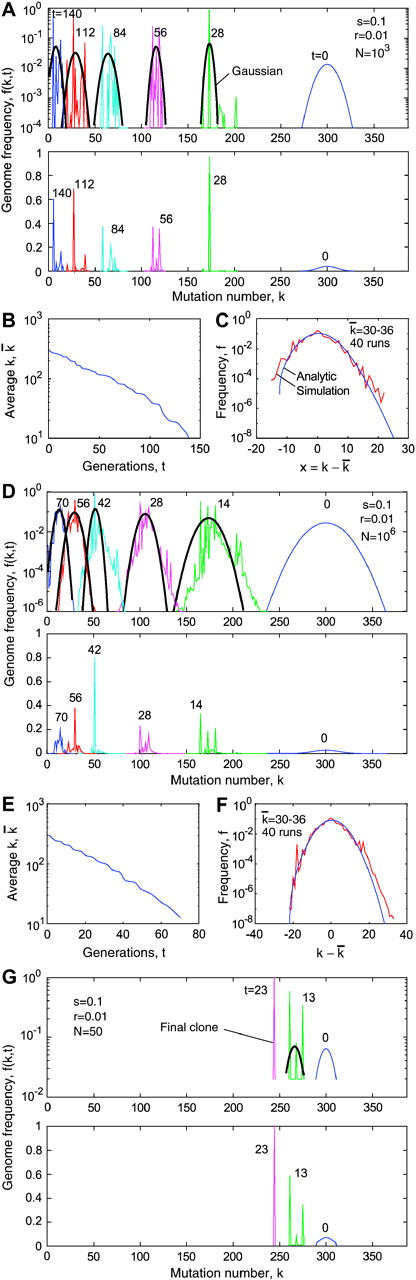
Monte Carlo simulation of the frequency of genomes with different mutation numbers f(k, t). (A) Lines in alternating colors: f(k, t) at different times (generations of infected cells) shown above the curves. Black line, fitting f(k, t) with a Guassian function; top and bottom, f(k, t) in logarithmic and linear scales, respectively. Model parameters are shown at the top. (B) Population-average mutation number as a function of time. (C) Wave profile (centered distribution of genomes over the mutation number) φ(x). Red line, simulation result averaged over the interval of shown at the top and over 40 random runs; blue line, analytic result (Equation 19). (D–F) Analogous results for a larger population size N. (G) Simulation below the critical population size, Nr < 1.

If we allow for a finite mutation rate μ, and r is small (r < 10⁻⁴), the accumulation rate below the critical point in population size may become finite. Figure 3 includes the analytical results obtained for an asexual population for parameter values relevant for HIV. [We used Equations 15, 16, and 19–21 in Rouzine et al. (2003) and estimated ξ ∼ for |v| ≪ /ln1/ from Equations 26 in the same work.] At large population sizes, the asexual accumulation rate is given by V_asex ≃ 2s lnNμ/ln²s/μ (Rouzine et al. 2003), which, in a broad range of N, is smaller than the recombination-driven rate by a large factor of . The result for the asexual rate remains valid until a population becomes exponentially large, lnNμ ∼ ln²s/μk; beyond this point, the rate is given by the one-locus result, . In contrast, the recombination-driven evolution rate given by Equation 1 reaches 50% of the one-locus rate already at N ∼ 1/rs/r². Therefore, at large , even very modest recombination is more efficient for generating highly fit genomes than mutation (provided the necessary more-fit alleles exist in the beginning).

Implication for HIV evolution and antiretroviral therapy:

The time to drug resistance depends on the number of antiretroviral drugs used in therapy. To give a general idea about the magnitude of this effect, we use an example of parameter values typical for an HIV infection in vivo: the mutation rate for transitions, μ = 3 × 10⁻⁵ (Mansky and Temin 1995); the average effective population size in untreated patients, N_un = 10⁶ (Rouzine and Coffin 1999a; Frost et al. 2000); and r(N_un) = N_un/N₀ = 1 (upper estimate, Jung et al. 2002), implying N₀ = 10⁶. Drug-resistance alleles in untreated patients are slightly less fit than wild-type alleles; on the basis of reversion experiments, we assume, for these sites, s = 0.1. One generation of infected cells corresponds to 1 day.

Because N_unμ ≫ 1, a population contains genomes that are drug resistant at a single base, at a deterministic frequency given by μ/s = 3 × 10⁻⁴ (N_unμ/s = 300 copies). However, the proportion of patients that carry a genome with two resistant alleles is small, N_un(μ/s)² = 0.1; it is even smaller for three alleles, N_un(μ/s)³ = 3 × 10⁻⁵.

An onset of antiretroviral treatment depletes a (wild-type) population to a low number, N ≪ N_un. In the presence of drug, each resistant base in a genome increases the logarithm of fitness by s ∼ 1. An important parameter is the minimum number of resistant alleles per genome, k₀, required to reach the critical level of fitness, at which virus can start expanding back in the presence of drug (therapy failure). The value of k₀ correlates with (but is not equal to) the number of drugs in a cocktail targeting different sites and depends on details of drug binding and population dynamics (e.g., the increase in the target cell number during therapy). A therapy depending on a single base, k₀ = 1, such as 3TC treatment, fails rapidly in every patient due to outgrowth of preexisting mutants.

For k₀ = 2, which is the case with most current drug cocktails, failure will occur in the 10% of patients that have preexisting two-base mutants. For the remaining 90%, the outcome will depend on the population size under therapy (and, indirectly, on the drug dosage). A population is dominated by genomes with one resistant allele. Recombination or mutation can add a second allele. A single copy of a double mutant will be fixed rapidly in a population and cause immediate therapy failure. The average time to such event, t_res, is either 1/μN or 1/r(N)N, whichever is smaller. We call a therapy successful if t_res > 1000. Then, the condition of successful therapy, from either the recombination or the mutation time, is N < 30 (viremia <1 copy/ml serum). Indeed, the currently used high-dosage therapy either fails rapidly (in ∼10% of patients) or achieves long-lasting control of viremia at the level <5 copies/ml. The above estimate assumes that there is one possible site for each of the two alleles, and the two bases are sufficiently far apart (>1000 nt, the crossover length). If the bases are close, or if there is more than one possible site, the upper bound on N will, respectively, increase or decrease.

For k₀ = 3, virtually none of drug-naive patients have preexisting fully resistant genomes. In a typical patient, two consecutive recombination or mutation events have to occur. After the first event, a double-mutant genome expands rapidly to the entire population; a second event makes virus resistant. The success condition, by analogy with the previous case, is N < 45 (the first mutation can choose between two sites).

Suppose that the critical number of drug-resistance sites is large, k₀ ≫ 1 (for example, 20). Now, the early recombination events are not the limiting factor. As we find in this work, accumulation of beneficial alleles due to recombination will stop, if Nr(N) < 1, which yields N < ∼ 10³, which is higher by a factor of 30 than the estimate for k₀ = 2.

Resistant alleles can still accumulate due to mutation. The analysis, for this mechanism, is more complex, because it essentially depends on the value of s that depends, in its turn, on the drug concentration. At a large number of drugs, the value of s per site required to achieve the decrease in virus fitness necessary to maintain depletion of wild-type virus will be ≪1. Therefore, the asexual evolution rate will be small, as compared to the case k₀ ∼ 1 (see the previous section).

In any case, we can conclude that the net drug concentration required to prevent rebound of resistant strains can be significantly decreased, if the number of target sites in the HIV genome is large.

In our early work (Rouzine and Coffin 1999b), we used a one-locus deterministic model to interpret evolution of reverse transcriptase in chronically infected untreated patients. The extrapolated average number of diverse sites per genome per patient is 100–300; on the average, these bases are highly diverse (25%). We proposed that these bases are, at the typical sampling time t ∼ 1000, in the middle of reversion to better-fit variants and estimated s ≈ 0.01. According to our present findings, the reversion speed is given by the one-locus expression, if rN_un ≫ s ∼ 0.1. Even if the estimate r(N_un) ∼ 1 overestimates the coinfection frequency by a factor of 10, our new findings confirm the validity of our earlier approach.

ANALYTIC DERIVATION

The derivation presented in this section is asymptotically exact over a range of parameters, such that ≫ 1, s ≫ r, 1 < lnNr ≪ min, 1/s², s/r²ln s/r. We make use of these strong inequalities and neglect terms that represent small corrections. In several places (appendix, Note 1–Note 5), smallness of a term is verified after the derivation. Monte Carlo simulation (Figure 3) confirms that our use of the strong inequalities is appropriate for parameter values typical for HIV infection.

Deterministic equation for randomized loci:

We consider the case of infinite population size, N = ∞. Let f(k, t) be the average fraction of nucleotide sequences that have, as compared to the best-fit sequence that could evolve, k deleterious mutations. For the model illustrated in Figure 1, the continuity equation for f(k, t) has a form

3

where t is time measured in generations of infected cells; s is the selection coefficient; e^−st ≡ ∫dk · e^−skfk, t; r is the recombination parameter (for symmetric co-infection, equal to the probability that an infected cell is coinfected by another virus); rR(k, t) is the gain in sequences with k mutations due to recombination between other sequences, as defined below; and −rf(k, t) is the loss of sequences with k mutations due to recombination with other sequences. Functions f and R are normalized, as given by . Equation 3 neglects mutation events.

In the stated parameter range (model and results), we have s|k − | ≪ 1 for all relevant k (appendix, Note 1), so that the exponential in Equation 3 can be replaced with its linear expansion in k − . In addition, f(k, t) can be approximated with a function continuous in t (appendix, Note 2). As a result, we have

4

where t ≈ ∫dk · kfk, t is the average mutation number per genome.

The form of the recombination gain function R(k, t) in Equation 4 is determined from the model assumptions that a recombinant genome inherits 50% of each parental genome, and positions of k mutations are fully random within each genome. In this and the next five sections, we consider a population with a small frequency of less-fit alleles per locus. A more general case is considered in the end of this section. Recombination of two genomes with k₁ and k₂ mutations, respectively, makes a genome with k = (k₁ + k₂)/2 + ε₁ + ε₂ mutations, where ε₁₍₂₎ is the Poisson fluctuation of the mutation number in the copied half of a parental genome, restricted by the condition that the total mutation number in the genome is fixed and equal to k₁₍₂₎. The fluctuation variance is given by , where k₁₍₂₎/2 is the average number of mutations in half of a genome, and the additional factor ¹/₂ is due to the restriction. Since fluctuations in the two genomes are independent, and, in the stated parameter range, the width of the distribution in k is smaller than , |k₁ − k₂| ≪ (appendix, Note 3), we have . The resulting expression for R(k, t) has a form

5

Solitary wave solution:

A partial solution of Equation 4 describes a steady process in which the distribution function assumes an almost constant profile in k, as given by

6

The “solitary wave” solution, Equation 6, describes gradual reversion of mutant loci (accumulation of beneficial mutations) on sufficiently long timescales. Substituting Equations 6 into Equations 4 and 5, we get

7

8

where x ≡ k − , and V ≡ −d/dt is the solitary wave speed toward higher fitness (reversion/accumulation rate). In Equation 7, we neglected the time dependence of the wave profile, which is asymptotically correct, if the wave is far from the origin k = 0 (Note 4).

The general solution of Equation 7 has a form

9

where x₀ is an arbitrary integration constant to be determined later in this subsection, and we introduced the notation

10

11

At infinite population size, Equation 9 is supposed to apply at any x, even when φ(x) is very small. Therefore, we must have x₀ = −∞; otherwise the distribution function φ(x) will be negative at x < x₀. The solution of Equations 8 and 9, for which the integral in Equation 9 does not diverge at x′ = −∞, has the form

12

13

For the wave speed, V, we have

14

Equation 12 that can be verified by direct substitution into Equations 8 and 7 implies that the variance of k is equal to the Poisson value t, i.e., that, in the limit of infinite population size, loci evolve independently. Below we show that, if the recombination parameter r is large, loci are independent at finite N as well. Equation 14 is a well-known deterministic result for the average reversion rate in the presence of selection.

Finite populations—solitary wave profile has an end:

At finite N, the number of sequences in each group Nφ(x) is a finite integer and, naturally, cannot be less than one. Small groups of sequences near the edges of the solitary wave are destroyed by random drift, i.e., by random sampling of genomes that give progeny for the next generation. As a result, the wave can end at a finite negative x = x₀: at x < x₀, φ(x) ≡ 0. The value x ≈ x₀ corresponds to the best-fit sequences present in a population (Figure 2).

We assume that, at sufficiently large N, random drift can be neglected for groups of sequences with k located far from the wave edges and that Equation 9 holds in the ensemble-average sense. This assumption is equivalent to neglecting the correlation function δfk, tδ, where δf(k, t) and δ are random fluctuations of the corresponding quantities, in the right-hand side of Equation 3. Results of the Monte Carlo simulation show the accuracy of this approach for the average values of φ(x), V, and w² up to N as small as 100–1000 (Figure 3 and Figure 4, C and F).

At finite x₀, the integral in Equation 9 does not need to converge at x = −∞, and values of w² < are allowed. As we show below, (i) the left tail of distribution φ(x) is long, |x₀| ≫ w, and (ii) in most of the interval x₀ < x < |x₀|, the integral in x′ in Equation 9 is contributed from a small region near the edge, x − x₀ ∼ δx (appendix, Note 5). Therefore, in this interval of x, Equation 9 takes a Gaussian form,

15

16

where the second equation is the normalization condition for φ(x), and δx is defined in the appendix, Note 5. Thus, parameter w represents the standard deviation of sequences in k, i.e., a characteristic width of the wave profile φ(x). It is smaller than the Poisson value due to linkage.

Substituting Equation 15 into Equation 8 and integrating over x₁ and x₂, for the recombination-gain function we obtain

17

which is valid at any x. [We can use asymptotics (15) for φ(x), because the integrals in x₁ and x₂ in Equation 8 converge at |x₁₍₂₎| ∼ w ≪ |x₀| (appendix, Note 5)].

The edge position x₀ can be expressed in terms of w using the normalization condition, Equation 16. Substituting Equation 17 into Equation 16, expanding the logarithm of integrand in Equation 16 linearly in x′ − x₀ (Note 5), and integrating in x′, we obtain

18

where we have neglected logarithmic factors in the argument of the large logarithm.

In the low-fitness tail, x > |x₀|, the integral in Equation 19 is contributed mostly from the region x′ ≈ x, and φ(x) decays like ρ(x) given by Equation 17, i.e., more slowly than it does at 0 < x < |x₀|.

Substituting Equation 17 into Equation 9 yields

19

20

Equation 19 is more general than the Gaussian asymptotics (Equation 15), because it is valid at any x > x₀. Altogether, the function φ(x) has four important characteristic intervals in x: (i) x < x₀, where it is zero; (ii) 0 < x − x₀ ≪ δx (Note 5), where Equation 19 predicts φ(x) ∝ x − x₀; (iii) the central interval |x₀| − |x| ≫ δx, where φ(x) is given by the Gaussian asymptotics, Equation 15; and (iv) x > |x₀|, where φ(x) ∝ ρ(x), Equation 17.

Equation 18, obtained within a deterministic approach, relates the cutoff length, |x₀|, to the standard deviation, w (that also defines the solution speed, Equation 11). To obtain a second equation for the two parameters, we have to consider stochastic effects at the high-fitness edge of the wave.

Stochastic high-fitness edge:

The extension of the high-fitness edge in time is illustrated in Figure 2. We use a two-variant argument considering a clone forming near the edge as a minority variant with an effective selection coefficient and the other genomes in the population as the majority variant. Recombination creates a single copy of a genome in a group beyond the edge, x < x₀, with a small probability of rNρ(x) per generation. As we show below in this subsection, at sufficiently large N, we have |x₀| ≫ . Most genomes outside of the wave are produced in a small region near the edge with a width Δ given by

21

The total rate of genome production, in this region, is G ∼ rNρ(x₀)Δ. After a sequence is produced, it will, most likely, become extinct in a few generations. If it survives and grows into a clone exceeding a characteristic size, fN ∼ 1/S, which event has a probability ∼S (Rouzine et al. 2001), the clone will be amplified by selection and become a part of the solitary wave. The average time to seeding a successful clone is

22

where we have substituted Equation 21 for Δ and Equation 17 for ρ(x₀) into the expression for G. On the other hand, the time to successful seeding must be equal to the time in which the solitary wave moves by Δ, as given by

23

where we used Equations 11 and 20 for V and Equation 21 for Δ. From Equations 22 and 23, we obtain the desired second equation for x²₀,

24

where we have neglected a logarithmic factor in the argument of the large logarithm. Within the same accuracy, solving Equations 18 and 24 for x²₀ and p, we arrive at Equation 1 that represents the main result of this work.

The validity of the above derivation is limited, in particular, by the condition Nr ≫ 1. At Nr ∼ 1, from Equations 24 and 21, we have |x₀| ∼ , Δ ∼ |x₀|, so that our assumption that new clones are generated near the high-fitness edge no longer holds. That a new clone is generated at a large distance from the wave implies that the old wave becomes extinct before it incorporates the new clone. Therefore, the new clone takes over the entire population. Because self-recombination of a single clone does not make any new genomes, the wave stops. We conclude that a critical point in Nr exists, (Nr)_c ∼ 1, below which the speed and the width of the wave are exactly zero. Interestingly, Equation 1 that does not need to be correct at Nr ∼ 1, nevertheless, extrapolates to V = 0 at Nr = 1.

Solitary wave consists of sparse clones:

The above derivation may appear inconsistent: the main part of the distribution f(k, t) is treated in the ensemble-average sense, as a continuous function in k, while the high-fitness edge is treated discontinuously and stochastically. In fact, each group with a given number of mutations is created as a clone (a group of identical sequences), at a distance from the high-fitness edge + x₀ − k ≫ 1. Therefore, at any one time and in any realization, an actual distribution of genomes over k is not continuous but consists of separate peaks representing clones, with gaps between them (Figure 4, computer simulation). Because clones are positioned randomly in k, as long as their total number is large, they average out into a continuous dependence (Figure 4, D and F). The form of the average simulated wave profile agrees with the analytic result with good accuracy, which demonstrates consistency of our approach.

Now we make some useful estimates pertaining to the clone structure of the wave. We start by estimating the number of clones that are created near the edge, x ≈ x₀. Because the growth of a clone, after it passes the stochastic bottleneck, is exponential in time, these edge-born clones are expected to grow to much larger sizes than the recombinant clones created inside the wave. The average distance in k between the large clones is the same as the initial distance of a new edge-born clone to the edge, ∼Δ, Equation 21. Therefore, the total number of large clones within a wave is given by

25

where we used Equations 24 and 21 and neglected a logarithmic factor inside a large logarithm.

The second estimate is of the average number of all clones at location x, G(x). A clone with k mutations can be generated in a time interval [t₁, t₂] given by the conditions . By analogy with the derivation under Stochastic high-fitness edge, G(x) is given by

26

Here dx′/V = dt is a small interval in time, the expression in brackets is the rate at which recombination generates genomes, and is the survival probability of a clone given by the effective selection coefficient. Using Equations 21, 22, 23, and 17, we get

27

If G(x) ≪ 1, parameter 1/G(x) yields the average distance in k between clones. We observe that clones tend to accumulate near the wave center x = 0, where the recombination gain ρ(x) is maximum. The total number of clones is given by

28

where we used Equations 22 and 23.

On the basis of Equations 25 and 28, we observe that, at Nr ∼ 1 [within accuracy of ln(s/r)], the numbers of all clones are on the order of 1. At this point, as we discussed, the wave degenerates into a single clone and stops. At Nr ≫ 1, we have M_tot ≫ M_lar ≫ 1; i.e., the distribution f(k, t) consists of a moderately large number of tall peaks corresponding to edge-born clones and more numerous smaller peaks corresponding to clones born inside the wave. The clone structure defined by Equations 25–28 can be used to measure experimentally the population size and other parameters.

Reversion of an almost uniform population:

In the previous sections, we considered the case when less-fit alleles are sparse and randomly located in the genome. In an experiment on drug-resistant strain evolution, an initial population consists of identical sequences with deleterious alleles at k₀ loci, with a small admixture of sequences carrying a beneficial allele at one of these loci. The average frequency of a beneficial allele at a locus, f₀, is assumed to be in the range 1/(Ns) ≪ f₀ ≪ 1, so that it exceeds the size of stochastic bottleneck, and random drift is not important for these groups of sequences. One the other hand, because 1 − f₀ ≃ 1, position of deleterious loci in different genomes mostly coincide, and the previous consideration based on Equation 5 does not apply directly.

Let us consider k₀ clones with a beneficial allele at one of k₀ loci that are deleterious in other sequences. The process of reversion consists of two stages: at the first stage, these sequences are amplified by selection over a timescale (1/s)ln[1/(k₀f₀)], until k₀ clones share population equally, so that . At the second stage, recombination of these clones drives the reversion process by collecting beneficial variants within a genome. Because recombination occurs by multiple and random template switches, positions of the few beneficial alleles among k₀ possible positions will become approximately random after several rounds of recombination and amplification. Therefore, while beneficial alleles are few, k₀ − ≪ k₀, we can use Equation 5 for the recombination gain function ρ, in which is substituted by k₀ − . As time goes on, the wave moves toward smaller , and a good proportion of formerly mutant loci will become better fit, k₀ − ∼ k₀. Therefore, we have to use a more general replacement,

29

that corresponds to the random distribution of beneficial alleles over k₀ available positions.

In the previous case /k₀ ≪ 1, parameter enters the problem only through the function ρ (Equation 5). Therefore, all the previous results apply after the replacement, Equation 29.

COMPUTER SIMULATION

Thus, we obtained analytic expressions for the ensemble-average properties of an evolving population. To test these results further, and to connect them to stochastic evolution in a separate realization, we undertook a Monte Carlo study. We considered a population with a small frequency of deleterious alleles. We have used the same approach to recombination as described above (assuming random distribution of alleles within a genome), with one correction. To account for the fact that recombination within a clone has zero effect, we assumed that a group with k mutations does not recombine with itself.

The approach is valid, because and, therefore, the width of the wave w given by Equation 1 are large (except near the critical point, where p ∼ 1/). At moderate or small Nr, the wave in each realization consists of rare groups with sparse k (see section above; Figure 3). Sparsity of groups implies automatically that most of them represent separate clones that grew from infrequent recombinants. The probability that an isolated group consists of, e.g., two clones is as small as 1/Δk, where Δk is the average spacing between two neighbor groups. Therefore, in this case, the exclusion of self-recombination of a group is approximately identical to exclusion of self-recombination of a clone. As N decreases, the number of clones becomes smaller, and the correction becomes more and more important. In contrast, at very large Nr, the wave consists of groups densely situated at adjacent k. The correction, in this case, is incorrect, because each group consists of many clones; however, it is also small, because the probability that a recombining genome recombines with another genome with exactly the same k is small, ∼1/w ≪ 1.

In our simulation, we stored the (integer) number of sequences with k mutations at each generation t, n(k, t) = Nf(k, t). At each generation change, we calculated the expected value nk, t + 1 for all k = 1, … , L, using the deterministic equation, Equation 3, with the recombination gain function R(k, t), Equation 5, corrected for the absence of self-recombination and normalized to 1. All groups with nk, t + 1 smaller than a set small value n_emp ≪ 1 were declared “empty in the next generation.” Then, we generated new numbers of sequences for nonempty groups, n(k, t + 1), by one of two methods.

1. If the average size of a group, nk, t + 1, was smaller than a set number n_stoch ≫ 1, and the total fraction of such groups was less than a set value f_tot < 1, we considered these groups “stochastic” and generated pseudorandom Poisson numbers n(k, t + 1) with the averages nk, t + 1. The remaining large groups were treated deterministically by setting .

2. If the total fraction of the stochastic groups exceeded f_tot, we treated all nonempty groups stochastically, as follows. We generated N random points in the interval [0, 1] separated into subintervals, each interval corresponding to a group k, with its width proportional to nk, t + 1. The new number n(k, t + 1) was set to be the number of random points falling within interval k. We checked that choosing n_emp < 10⁻⁴–10⁻⁵, n_stoch > 500–1000, and f_tot < 0.2 did not change the results significantly.

The method described above was designed to enhance the speed of the algorithm without a significant loss in accuracy. We were able to simulate populations with as large as 500 and arbitrarily large N.

After each Monte Carlo run, we calculated the time dependence of the average mutation number t, the logarithm of the accumulation rate , the normalized average variance w²t/t, and the centered wave profile . Then, we averaged the three values over a time interval, such that ₀ < t < 1.2₀, where ₀ was a “sampling” mutation number, and then over 10–40 computer runs. We verified that using a shorter time interval for averaging did not affect our results, because, on the average, ln V and w²t/t changed slowly in time. Due to the additional averaging over the time interval, the modest number of random runs (10–40) was sufficient to ensure, for most points in N, a small statistical error for the estimate of the average value of p (Figure 3, ≤0.1). To minimize the transitional period to a steady-moving wave, we used the analytic result, Equation 15, as the initial condition f(k, 0). We verified that choosing the initial wave center at was sufficient to decrease the remaining effect of initial conditions below the statistical error.

Examples of simulated dependences fk, t and t are shown in Figure 4; we discussed them previously. The ensemble-average reversion rate and the wave width square , normalized to the respective deterministic (independent-loci) values s₀ and ₀ for different values of model parameters, are shown in Figure 3. In agreement with the analytic theory (Equation 11), the values of V_av/s₀ and w²_av/₀ are very close. We also observe that simulation confirms the existence of a critical point in Nr, where the reversion speed becomes zero, and that the analytic dependence V(N) (Equation 1) is reproduced with a sufficient accuracy to be practically useful. At large recombination parameters, r > s, a steep increase in V_av/s from 0 to 1 occurs at Nr ∼30 (Figure 3).

Conclusion:

We have obtained an asymptotically accurate expression for the accumulation rate of beneficial mutations for the case where small amounts of beneficial alleles exist in the beginning, and mutation can be neglected. On the basis of our findings, we predict that depletion of an HIV population by antiretroviral therapy below a critical size will suppress accumulation of drug-resistant mutations. When beneficial alleles do not preexist in a population, mutation and recombination are expected to work together, and alternative formalism has to be developed. We plan to carry out this task elsewhere.

APPENDIX

Note 1:

In Equation 4, we assumed that, for all relevant k, s|k − | ≪ 1. Because the far low-fitness tail is not essential, it is sufficient to check this condition at the high-fitness edge, . Using Equation 24 for x₀, we obtain the validity condition

A1

Note 2:

In Equations 4 and 7, we assumed that f(k, t) can be approximated with a function continuous in t, which implies V|d ln φ/dx| ≪ 1. At negative x, |d ln φ/dx| reaches its maximum at x ≈ x₀ (Equation 15), where we have

A2

where we used Equations 1 for V and w and Equation 24 for x₀. The resulting validity condition has the form of inequality (A1).

Note 3:

In Equation 5, we assumed that the solitary wave is narrow compared to the distance from the origin, as given by |x₀| ≪ . Using Equation 24 for |x₀|, the validity condition becomes

A3

Note 4:

When calculating ∂f/∂t in Equation 7, we neglected the implicit dependence of φ on t. This action is justified, if

A4

From Equations 20 and 1 we get

A5

From Equation 15 we have

A6

Substituting (A5) and (A6) into inequality (A4) and using , inequality (A4) takes a form |x| ≪ . The sufficient condition is obtained at x = x₀, which yields the narrow wave condition, inequality (A3).

Note 5:

When deriving Equation 15, we assumed that |x₀| ≫ w; i.e., the high-fitness tail of the distribution is longer than its characteristic width. Using Equations 18 and 11, we have |x₀|/w ∼ ln^1/2s/r, which is ≫1, if 1 − p ≫ r/s²/. Using Equation 1, the validity condition takes a form

A7

We also assumed that, over most of the interval |x| < |x₀|, the integral in x′ in Equations 9, 16, and 19 is contributed from a small region, x′ ≈ x₀. Indeed, at |x₀| − |x| ≫ δx, where δx ∼ p/1 − p|x₀|, the integral in Equation 19 is mostly contributed from a region x′ − x₀ ∼ δx. Using Equation 18, we have δx/|x₀| ∼ ln⁻¹s/r ≪ 1, which, again, yields inequalities (A7).

References

- Barton, N. H., 1995. A general model for the evolution of recombination. Genet. Res. 65: 123–144. [DOI] [PubMed] [Google Scholar]
- Barton, N. H., 1998 Why sex and recombination? Science 281: 1986. [PubMed]
- Felsenstein, J., 1974. The evolutionary advantage of recombination. Genetics 78: 737–756. [DOI] [PMC free article] [PubMed] [Google Scholar]
- Fisher, R. A., 1930 The Genetical Theory of Natural Selection. Clarendon Press, Oxford.
- Frost, S. D., M. Nijhuis, R. Schuurman, C. A. Boucher and A. J. Brown, 2000. Evolution of lamivudine resistance in human immunodeficiency virus type 1-infected individuals: the relative roles of drift and selection. J. Virol. 74: 6262–6268. [DOI] [PMC free article] [PubMed] [Google Scholar]
- Hey, J., 1998. Selfish genes, pleiotropy and the origin of recombination. Genetics 149: 2089–2097. [DOI] [PMC free article] [PubMed] [Google Scholar]
- Hill, W. G., and A. Robertson, 1966. The effect of linkage on limits to artificial selection. Genet. Res. 8: 269–294. [PubMed] [Google Scholar]
- Jung, A., R. Maier, J. Vartanian, G. Bocharov, V. Jung et al., 2002. Multiply infected spleen cells in HIV patients. Nature 418: 144. [DOI] [PubMed] [Google Scholar]
- Levy, D. N., G. M. Aldrovandi, O. Kutsch and G. M. Shaw, 2004. Dynamics of HIV recombination in its natural target cells. Proc. Natl. Acad. Sci. USA 101: 4204–4209. [DOI] [PMC free article] [PubMed] [Google Scholar]
- Mansky, L. M., and H. M. Temin, 1995. Lower in vivo mutation rate of human immunodeficiency virus type 1 than that predicted from the fidelity of purified reverse transcriptase. J. Virol. 69: 5087–5094. [DOI] [PMC free article] [PubMed] [Google Scholar]
- Muller, H. J., 1932. Some genetic aspects of sex. Am. Nat. 66: 118–128. [Google Scholar]
- Otto, S., and N. Barton, 1997. The evolution of recombination: removing the limits to natural selection. Genetics 147: 879–906. [DOI] [PMC free article] [PubMed] [Google Scholar]
- Rouzine, I., J. Wakeley and J. Coffin, 2003. The solitary wave of asexual evolution. Proc. Natl. Acad. Sci. USA 100: 587–592. [DOI] [PMC free article] [PubMed] [Google Scholar]
- Rouzine, I. M., and J. M. Coffin, 1999. a Linkage disequilibrium test implies a large effective population number for HIV in vivo. Proc. Natl. Acad. Sci. USA 96: 10758–10763. [DOI] [PMC free article] [PubMed] [Google Scholar]
- Rouzine, I. M., and J. M. Coffin, 1999. b Search for the mechanism of genetic variation in the pro gene of human immunodeficiency virus. J. Virol. 73: 8167–8178. [DOI] [PMC free article] [PubMed] [Google Scholar]
- Rouzine, I. M., A. Rodrigo and J. M. Coffin, 2001. Transition between stochastic evolution and deterministic evolution in the presence of selection: general theory and application to virology. Microbiol. Mol. Biol. Rev. 65: 151–185. [DOI] [PMC free article] [PubMed] [Google Scholar]