Incorporation of Competitive Effects in Forest Tree or Animal Breeding Programs

Abstract

Competition among domesticated plants or animals can have a dramatic negative impact on yield of a stand or farm. The usual quantitative genetic model ignores these competitive interactions and could result in seriously incorrect breeding decisions and acerbate animal well-being. A general solution to this problem is given, for either forest tree breeding or penned animals, with mixed-model methodology (BLUP) utilized to separate effects on the phenotype due to the individuals' own genes (direct effects) and those from competing individuals (associative effects) and thereby to allow an optimum index selection on those effects. Biological verification was based on two lines of Japanese quail selected for 6-week weight; one line was selected only for direct effects (D-BLUP) while the other was selected on an optimal index for both direct and associative effects (C-BLUP). Results over 23 cycles of selection showed that C-BLUP produced a significant positive response to selection (b = 0.52 ± 0.25 g/hatch) whereas D-BLUP resulted in a nonsignificant negative response (b = −0.10 ± 0.25 g/hatch). The regression of percentage of mortality on hatch number was significantly different between methods, decreasing with C-BLUP (b = −0.06 ± 0.15 deaths/hatch) and increasing with D-BLUP (b = 0.32 ± 0.15 deaths/hatch). These results demonstrate that the traditional D-BLUP approach without associative effects not only is detrimental to response to selection but also compromises the well-being of animals. The differences in response show that competitive effects can be included in breeding programs, without measuring new traits, so that costs of the breeding program need not increase.

THEORIES on which most current plant and animal breeding selection methodologies were developed have generally ignored competitive interactions among individuals, specifically the impacts of the genes of one individual on the performance of other individuals. In plants such interactions reduce growth and yield due to competition for limited resources such as light, water, and nutrients. In penned livestock such interactions not only reduce growth and productivity, but also can result in injury and death, thereby raising concerns about the impact of current selection programs on animal well-being, an issue of increasing importance. Associative effects are defined as interactions among animals and can be due to a number of factors, including: competition for limited resources, social dominance, and pecking order; misdirected feeding behaviors such as some types of feather and vent pecking in chickens (Craig and Muir 1996); and, in the extreme case, cannibalism, as commonly seen in aquaculture (Kestemont et al. 2003).

Falconer (1981) briefly mentioned the impact of competition on the resemblance between relatives and noted that the intraclass correlation could be reduced by competition and even become negative. Falconer (1981)(p. 146) concluded that “Competition is an important factor in plants, often making sib-correlations largely meaningless, particularly with characters related to yield.” If the correlation among sibs is meaningless, then advantages of selection programs utilizing resemblance between relatives, such as best linear unbiased prediction (BLUP) (Henderson 1985; Sorensen and Kennedy 1986; Lynch and Walsh 1998; and references therein), would also be greatly reduced or eliminated.

Unfortunately there have been few, if any, controlled selection experiments in which the relative efficiency of BLUP has actually been compared to mass selection. A number of earlier experiments failed to confirm the theoretical advantages of a simpler version of BLUP: index selection (single trait, combining information from limited relatives) over mass selection (Kinney et al. 1970; Doolittle et al. 1972; Wilson 1974; Campo and Tagarro 1977; Garwood and Lowe 1979, 1980; Perezenciso and Toro 1992). In some of these experiments, e.g., Wilson (1974), index selection was worse than mass selection. One possible explanation was the increased rate of inbreeding associated with increased accuracy of selection index programs (Quinton and Smith 1995; Muir 1997). Another possible explanation is that competition was a factor and not only eliminated any advantage of using the index, but also was actually a detriment.

In forest tree breeding Wright (1977) demonstrated theoretically that with competitive effects, selection will result in a nonlinear response and become progressively less effective until a plateau is reached, beyond which selection would be detrimental. Competitive interactions are also an important source of variation for other plants. Denison et al. (2003) concluded that future genetic improvement of crop yield will involve tradeoffs between individual competitiveness and the collective performance of plant communities.

Reduced efficiency may not be evident in cases where management techniques are used to mitigate results of competitive interactions, such as beak trimming and dim lighting in poultry and tail docking in swine. If such practices are discontinued, due to concerns for animal well-being, as is the case in Europe (Council Directive 1998, 1999), then social interactions become an important part of the selection response. If such selection programs increase animal suffering and mortality, they may be banned by the European Union Council ( Council Directive 1998) under Directive 20, “Natural or artificial breeding or breeding procedures which cause or are likely to cause suffering or injury to any of the animals concerned must not be practiced,” and Directive 21, “No animal shall be kept for farming purposes unless it can reasonably be expected, on the basis of its genotype or phenotype, that it can be kept without detrimental effect on its health or welfare,” and create ethical concerns elsewhere. This concern was demonstrated by Craig and Muir (1996), who observed that a commercial line of poultry layers, undergoing continued selection for increased egg production, was either best or worst for egg production and survivability, as compared to a nonselected control, if the birds were not beak trimmed and were housed in single- or multiple-bird cages, respectively. Currently the only apparent alternatives to improve animal well-being are management related and include reducing housing density, eliminating some types of housing, and in some cases returning to free-range rearing. Such management practices are extremely inefficient and ignore the alternative possibility that animal behavior can be altered such that intensive management practices can be utilized without compromising animal well-being.

Few studies, however, have been conducted to evaluate whether selection for both improved animal performance and well-being can be attained. The objective of this article is to examine and compare alternative methods of incorporating competitive interactions in plant and animal breeding programs. Comparisons are based on theory, simulations, and a biological experimentation using Japanese quail.

THEORY

Extending the genetic model:

Griffing (1967) developed a theoretical framework to accommodate interacting genotypes in breeding programs. Griffing (1967) recognized that with competition, the usual gene model for a given genotype must be extended to include not only the direct effects of its own genes, but also the associative contributions from other genotypes in the group. To accommodate associative effects, Griffing (1967) extended the conceptual biological model to include not only direct effects of an animal's own genes, but also the associative contributions from other genotypes in the group.

Using the expanded model, for random groups of size n, Griffing (1967) showed that in the presence of interacting genotypes the expected change in the mean from selection on individual records is

1

where n is the group size, σ is the phenotypic standard deviation, i is the standardized selection differential, σ²_d is the additive genetic variance of the direct effects, and σ_ad is the additive genetic covariance between the direct and associative effects. If the covariance between the direct and associative effects is negative, as would occur with competition for a limited resource, then selection based on individual performance can have a reverse effect on the mean; i.e., positive selection will reduce rather than increase the mean. This results because a gene that has a positive direct advantage for the individual has a negative associative effect on records of other members of the group.

In contrast, if the group is defined as the unit of selection, then for groups of size n,

2

where gr indicates that i and σ relate to group means, and σ²_a is the additive genetic variance for associative effects. In this case Δμ is always positive. Thus, transferring selection from the individual record to the mean of the group ensures that the population mean will not decrease. As group size increases, associative effects will take on an increasingly dominant role in determining the consequences of selection, which implies that even for weakly competitive conditions, a negative response to selection can occur. This result was shown experimentally by Muir (1996), using poultry layers in which genotype-by-group-size interactions occurred between single- and nine-bird cages but not between single- and four-bird cages, with density held constant.

Group selection:

The term group selection has many different meanings and has sparked numerous debates. Wilson (1983)(p. 159) concluded that in the 1960s “group selection rivaled Lamarkianism as the most thoroughly repudiated idea in evolutionary theory.” The controversy is partially a matter of semantics. What some have called group or kin selection (Hamilton 1964; Wynne Edwards 1986) is actually selection among individuals for those individuals that would benefit the group. What others have called group selection is selection among groups, where the entire group is selected or culled on the basis of the performance of the group as a whole. The controversy stems from the first definition or as Wilson (1983)(p. 162) stated “if natural selection favors individuals that leave the most offspring, then individuals that benefit themselves at the expense of others should be very fit indeed. Individuals that benefit others, presumably at some expense to themselves, would be selected against as surely as if they had bad eyes or faulty teeth.” On the other hand, true group selection requires that natural populations be subdivided into groups such that selection could be among those groups. Maynard-Smith (1976) suggested that the term “group selection” be restricted to cases in which the group was the unit of selection. For clarity, the term group selection is used henceforth to refer to selection among groups, with the group as the unit of selection.

Controversy persists as to the role of group selection in evolution because group level adaptation requires natural selection among alternative groups but others argue that selection within groups will be opposed to that between groups (Williams 1966). Further controversy exists as to whether such grouping actually occurs in nature given that migration frequently occurs between groups (Wilson 1983). While these controversies are of interest to evolutionary biologists, for plant and animal breeders they do not have the same relevance because the breeder controls group size, structure, and the mating system.

Wade (1976)(1977), utilizing the red flour beetle (Tribolium castaneum), was the first to empirically demonstrate the effectiveness of group selection with randomly formed groups. Wade (1976)(1977) selected groups for either increased or decreased number of adults produced within the group and found that selection was effective in both directions, confirming that kin groups were not essential for group selection to be effective, and thus also confirmed the theoretical predictions of Griffing (1967). The first experiment to contrast individual with group selection was that of Goodnight (1985), who showed that leaf area of Arabidopsis thaliana responded to group but not individual selection. Several other experiments with laboratory insects have also clearly demonstrated the power of group selection to improve survival (Wade 1976, 1977, 1978; McCauley and Wade 1980; Wade and Mccauley 1980; Craig 1982).

Griffing (1976a)(b) later showed, theoretically, that group selection becomes more efficient as the average relationship within groups increases. The first selection experiment with groups composed of related individuals (half-sib families) was reported by Muir (1996), using poultry layers. Muir (1996) reported that after six generations of selection for annual egg mass produced by the group in multiple-birdcages, in comparison to the unselected control also housed in multiple-birdcages, annual percentage of mortality of the selected line (kinder, gentler bird, KGB) decreased from 68% in the initial generation to 8.8% in the sixth generation, which was similar to that of the nonselected control (C) in single-bird cages (9.1%).

Craig and Muir (1996) compared the selected and control lines to a commercial line, Dekalb XL (DXL), in generation 7 with hens again housed in either single- or 12-bird cages and under management conditions the same as in previous generations, except that birds that died were replaced with birds of the same line. Performance was measured from 20 to 58 weeks of age. In single-bird cages, performances in terms of eggs per hen housed, eggs per hen per day, egg weight, and egg mass were significantly greater for the DXL than for the KGB line, which in turn was greater than those for the C line. Mortality was zero for all three lines. However, in 12-bird cages a reverse ranking for performance was seen with the KGB line superior to the DXL line for eggs per hen housed, egg mass, and eggs per hen per day. The most remarkable difference was for mortality. The DXL line had 89% mortality at 58 weeks of age as compared to the KGB line with 20% and C with 54% mortality. The comparison to DXL is particularly important because this line constituted one of the resources used to establish the control line from which the KGB line was established. The DXL line resulted from continued selection for improved productivity based on individual bird performance. These comparisons demonstrate that continued selection on individual productivity will improve productivity when competitive interactions are absent, as in a single-bird cage, but can result in negative response to selection in group settings.

These results also demonstrate a classic genotype-environment interaction. Such interactions were predicted by the theories of Griffing (1967) and arguments of Williams (1966) whereby group adaptation requires group selection and individual adaptation will be opposed to those of the group.

Alternatives to group selection:

Griffing (1969) showed that group selection does not weight the information optimally for maximal genetic gain in group performance and is inefficient, particularly if groups are composed of random individuals. Increased efficiency can be obtained by forming nonrandom groups of related individuals. For optimum progress, however, Griffing (1969) concluded that an index is needed. Group selection is based entirely on between-group variation and ignores within-group variation. The optimal index would separate the direct and associative effects and weight each according to the variance-covariance structure of the genetic parameters, as per classic selection index theory. At that time Griffing's (1969) index could not be implemented because methods were not available for estimating genetic parameters needed to formulate the index or for separating each individual's direct and associative effects. The objectives of this research are to present methods to estimate the necessary genetic parameters, to estimate the direct and associative effects of each individual, and finally to demonstrate the efficacy of the index method, as an alternative to group selection, with a biological example using quail.

Competition by distance:

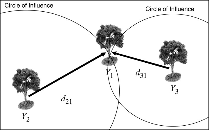
Consider first an application to forestry because this example represents the most general application of this approach. Clearly plants do not have a social component and compete only for limited resources. Let three trees exist in proximity to each other as given in Figure 1, with phenotypes Y₁, Y₂, and Y₃, and with distances between tree 1 and tree 2 of d₂₁ and between tree 1 and tree 3 of d₃₁. Assume that the degree of competition between plants is some function of distance. Without loss of generality, assume that plants compete equally well in all directions, with the greatest intensity directly beneath the plant and diminishing by the square of the distance (or some other to be determined function); i.e., the nutrients and resources collected are proportional to the density of leaves and roots, which by the branching nature of trees diminishes geometrically from the center. The actual rate at which competitive effects diminish may differ by species and should be verified by experimentation. Thus the influence of tree i on tree j is proportional to

3

where A^p_i is the phenotypic associative effect of tree i, which has a genetic and environmental component,

4

In the above example, the phenotype of tree 1 is described by the model

or

or

5

In general for t trees in a stand, the phenotype of each is influenced by all trees in the stand, but to varying degrees depending on distances and phenotypes of those trees:

6

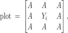
This model is an oversimplification as it ignores intervening trees, although the distance function would automatically give lesser impact to trees that are further away. If the trees are planted in rows, one alternative is to include only those trees that surround a given tree. With equal spacing this would result in a maximum of eight competing trees as is the case for the tree in the center of the following plot:

Similar adjustments can be defined for other planting arrangements and for along the edges or corners of the stand.

Figure 1.—

Relationship of three trees in a field.

Because there are three times as many effects to estimate as there are equations, simple least-squares solutions will not work. A general solution can be found using a mixed-model approach along with the additive genetic relationship matrix (G). While not exact, the additive genetic relationship can be thought of as a measure of partial genetic replication (closeness) between any two individuals; i.e., a relationship of 0 indicates that the individuals are genetically distant [no identical by descent (IBD) alleles] while a 1 indicates closely related individuals (all alleles are IBD). We therefore have essentially two measures of distances, genetic and physical. In the absence of a pedigree, molecular band-sharing data can be substituted (see Lynch and Walsh 1998, Chap. 27 and references therein).

These distances along with prior estimates of the genetic parameters allow the effects to be solved for using the following mixed model. Effects for individuals in the stand with missing records, or others in the pedigree, can also be estimated. Let N be the number of observations with values on the phenotype and M be the number of individuals in the pedigree (including those with missing records),

7

where Y is a (N × 1) vector of individuals with phenotypes recorded, such as yield; β is an (N × 1) vector of fixed effects, such as stand age, location, or block; X is an (N × r) incidence matrix identifying which of the r fixed effects are associated with each observation; D is an (M × 1) vector of random genetic direct effects and includes all individuals in the stand, with or without recorded phenotypes, and all others in the pedigree; Z_D is an (N × M) diagonal incidence matrix; A^g is an (M × 1) vector of random genetic associative effects for all individuals in the pedigree; Z_A^g is an (N × M) incidence matrix with elements C_ij on the off diagonals and 0 on the diagonal and for any tree that either does not immediately surround the ith tree or was not in the stand (i.e., parents); A^e is an (N × 1) vector of random environmental associative effects; Z_A^e is an (N × N) incidence matrix similar to Z_A^g but contains only columns for individuals physically present in the stand; and ε is an (N × 1) vector of random environmental effects. For the example in Figure 1, assuming the mean is the only fixed effect, the equations for the mixed model for the three phenotypes are

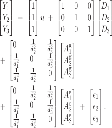8

The expectation of all random vectors is null while expected (co)variance is

9

Assuming a multivariate normal distribution, the derivatives of the logarithm of the likelihood with respect to all effects give the mixed-model equations (MME) multiplied by σ²_ε in Figure 2; the solutions are estimates of the fixed and random effects. The constants in the MME are found from Equation 10,

10

and

11

Under the assumptions of Equation 9, the Z_A^e term may be dropped from the model without loss of generality; the direct and associative environmental effects are then pooled. Solving for two environmental effects does not improve the estimates of the genetic effects, but for academic purposes may be useful to determine what the sources of environmental variation are, i.e., associated with competition or other.

Figure 2.—

Mixed-model equations (MME) to estimate direct and associative genetic effects.

Competition within a pen (animals):

Assume animals are randomly allocated to pens or cages and that all animals interact. This assumption may not be valid for some species and/or group sizes, particularly as the group size becomes large. Relaxation of these assumptions will be addressed in a future publication.

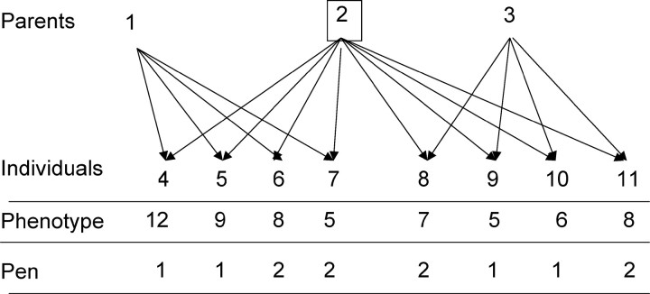
This situation is a special case of that with trees, because animals move about the cage and interact equally. Thus the physical distance for all animals in a common pen is a constant; for simplicity the distance is set to 1. For animals in different pens that are physically isolated and cannot interact, the distance is conceptually infinite so that the coefficient essentially becomes 0. Thus the coefficients in rows of matrices Z_A^g and Z_A^e are 1 if the animals are in the same pen and 0 otherwise. The remaining equations are the same as before. Consider the example given in Figure 3, with genetic parameters

The relevant matrices and SAS IML program to find the solutions are given in appendix A. The solutions are in Table 1. For large data sets more efficient programs are needed such as BLUPF90 (http://nce/ads.uga.edu/ignacy).

Figure 3.—

Example with related animals in common pens.

TABLE 1 .

Estimates of random genetic effects for the example in Figure 3

Individual	Direct genetic (Di)	Associative genetic (Ag)	Associative environmental (Ae)
1	0.464	−0.191	NA
2	0.000	0.000	NA
3	−0.464	0.191	NA
4	0.935	−0.327	−0.175
5	0.368	−0.094	0.024
6	0.328	−0.192	−0.106
7	−0.238	0.040	0.093
8	−0.201	0.025	−0.083
9	−0.721	0.409	0.315
10	−0.459	0.191	0.082
11	−0.012	−0.052	−0.150

The estimate of the overall mean was β₁ = 7.6.

Estimation of genetic parameters:

Relevant variance and covariance components can be estimated by restricted maximum likelihood (REML) and maximum likelihood (ML) (see Lynch and Walsh 1998, Chap. 27 and reference therein) or Bayesian methods, such as Gibbs sampling (Wang et al. 1993). A number of software packages are available for estimation of variance components via REML (see Spilke and Groeneveld 1994 for review and comparison) and Gibbs sampler (Van Tassell and Van Vleck 1996).

Optimum breeding programs—selection for direct and associative effects:

Once the direct and associative genetic effects have been estimated for each animal, the issue is how to combine them in a breeding program to make optimal progress. The solution is to use a selection index combining both traits and find optimal weights for each effect such that the performance of the group is maximized.

Define an index (I_i) for the ith individual as

12

where (b₁, b₂) are index weights and D̂_i and Â^g_i are the estimates of direct and associative genetic effects for the ith animal. The optimal weights are the contributions each effect has on the group mean. For groups of size n, each individual has one direct effect but (n − 1) associative effects on other records in the group. Thus the optimal linear index is

13

These weights show that even if the associative effects are small, in large groups the contribution of the associative effect to the index can be greater than the direct effect. Indeed, the net result may not be to increase direct genetic effects, but to decrease the negative associative effects.

Relative efficiency of alternative selection methods:

We have described two methods to improve group performance: (1) group selection, selection among groups based on the average performance of the group (in either random or kin groups), and (2) multitrait index selection among individuals within group (housed in either random or kin groups) based on direct and associative effects, estimated via mixed-model approaches. From the equations previously given, the relative efficiency of group vs. index selection is dependent on the average relationship within group, the relative magnitude of genetic variance for associative effects, and the genetic covariance between the direct and associative effects.

To examine the relative efficiency of these alternative methods under a variety of conditions, a gene level simulation program (Muir 2000) was utilized. Briefly the program allows for any number of chromosomes, any chromosome size, any number of loci per chromosome, any location on the chromosome, and any number of alleles per locus, all of which are drawn at random from a specified distribution (normal, uniform, or exponential). Recombination between loci is by distance based on Haldane's function. Following recombination, gametes are formed assuming independent Mendelian segregation of the chromosomes. Mutation rates, type of gene action (additive, dominance, epistasis), and pleiotropic effects (on up to two traits for each locus) are set by the user. The allele frequencies in the base population are randomly set and in Hardy-Weinberg equilibrium across the population; i.e., genotypic frequencies are products of the allelic frequencies. A large base population is then established, the genetic variance is computed, and a random environmental effect is added to each individual such that the desired heritability results. Direct and associative effects were simulated as two traits with some loci having pleiotropic effects for both. The phenotype of each individual was then computed as the direct genetic effect of its own genes plus the associative genetic effects of those animals in the same pen plus a random environmental effect.

Four methods of selection were compared: (1) group selection with groups composed of full sibs (K), (2) group selection with groups composed of random individuals (R), (3) individual selection using a model with only direct effects (D), and (4) individual selection with a model as described in Equation 7, but without associative environmental effects, Z_A^e (C).

Two sets of parameters were used in the simulations that differed only in the magnitude of the variance of the associative effects; i.e., the ratio of direct effects to environmental variance was constant, as was the genetic correlation between the direct and associative effects. These parameters are given in Table 2.

TABLE 2 .

Relative efficiency of selection using alternative selection methods

Magnitude of associative effects	Methoda	Response per generation	SE	Relative efficiencyb
Largec	C	0.721	0.021	3.03
	D	−0.229	0.004	−0.96
	K	0.509	0.011	2.13
	R	0.238	0.002	1.00
Smalld	C	0.098	0.002	3.69
	D	0.054	0.001	2.00
	K	0.078	0.002	2.88
	R	0.027	0.001	1.00

^aC, competitive effects BLUP, two random effects model; D, animal model with direct effects only; K, group selection composed of kin; R, group selection composed of random individuals.

^bRelative to R.

^c.

^d.

For C- and D-selection, BLUP was used to estimate genetic effects. The true values of the parameters were used in both C- and D-MME (given in Table 2). D-BLUP is traditional animal model BLUP, for which the associative genetic variance was combined with the environmental variance for the MME.

For all cases, the population size was 512, formed into 32 groups of size 16. For C-BLUP, the estimates of direct and associative genetic effects were combined using the index in Equation 13. Individuals were ranked on this index. For D-BLUP individuals were ranked on the direct genetic effect. For group selection (GS), K-GS and R-GS, groups were ranked on the basis of the groups' average. For each method, 32 males and 32 females were selected on the basis of the ranks. For K- and R-GS, all males and females in the top four groups were selected. The selected males and females were randomly mated. Each female produced 16 offspring, 8 of each sex. For method K-GS, full-sib families were housed together as a group. For all other methods, individuals were randomly assigned to groups. This process was repeated for 10 generations. The entire process was replicated 20 times for each method, starting over with a new sample of individuals for each replicate.

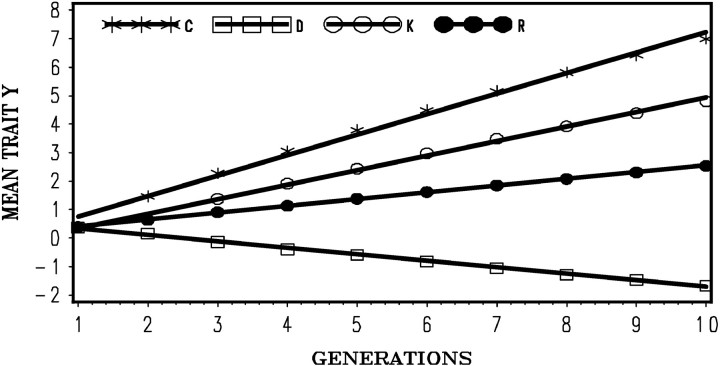
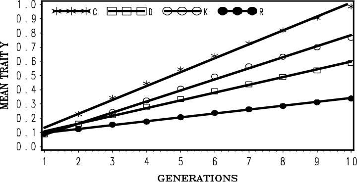
Rate of response to selection for each combination of parameters was estimated as the regression of the phenotypic means, averaged over replicates, on generation number. Relative efficiency was calculated as the ratio of rate of response for that method relative to R-GS. Results are given in Figures 4 and 5 for strong and weak associative effects, respectively. Regression coefficients for response per generation and relative efficiencies are given in Table 2.

Figure 4.—

Selection response over generations with alternative methods of selection and strong competitive effects : C-BLUP, index selection on direct and associative effects; D-BLUP, selection on direct effects only; K-GS, group selection, groups composed of full-sib individuals; R-GS, group selection, groups composed of random individuals.

Figure 5.—

Selection response over generations with alternative methods of selection and weak competitive effects : C-BLUP, index selection on direct and associative effects; D-BLUP, selection on direct effects only; K-GS, group selection, groups composed of full-sib individuals; R-GS, group selection, groups composed of random individuals.

When associative effects are large, selection on only the direct effects (D-BLUP) results in a negative response to selection. As expected, the most efficient method was index selection (C-BLUP), over three times as efficient as group selection in random groups (R-GS), while group selection in full-sib groups (K-GS) was 213% more efficient than in R-GS. When associative effects are weak, C-BLUP remains superior to all others, while D-BLUP produced a positive response and surpassed R-GS by 200% but is still inferior to K-GS. These results clearly demonstrate that index selection is superior in all cases, even when competitive effects appear small and traditional selection brings about a positive response to selection. The second-best alternative in both cases was group selection composed of full-sibs. Group selection in random groups, R-GS, always brings about a positive response to selection but is very inefficient when associative effects are small. Individual selection in random groups (D-BLUP) is always less than optimal and can be detrimental if associative effects are large.

Impact of group size on precision of estimates:

As group size increases, the number of interactions among animals also increases, so that effects may be more difficult to estimate in large than in small groups. Again, a simulation program was utilized to address this issue. Comparisons were based on the correlation between true and estimated breeding values for direct and associative genetic effects. A 2 × 2 × 2 factorial arrangement of group size (4 vs. 16) and genetic parameters were examined. For genetic parameters associative and environmental effects were set to be either large or small as shown in Table 3, with the correlation between direct and associative genetic effects held constant. The number of progeny each generation was 256, which were randomly assigned to pens of group size 4 or 16. For each group size phenotypes were recorded and 16 males and 32 females were chosen at random as breeders. These breeders were randomly mated, 1 male to 2 females, to produce the next generation for a total of 10 generations.

TABLE 3 .

Group sizes and genetic parameters used in the simulations

	Variance		Genetic parameters
Group size	Environmental	Associative effect	σ2D	σDA	σ2A	σ2E
4	Large	Large	72	−49	122	18
4	Large	Small	70	−9	7.5	18
4	Small	Large	72	−49	122	170
4	Small	Small	70	−9	7.5	170
16	Large	Large	72	−49	122	18
16	Large	Small	70	−9	7.5	18
16	Small	Large	72	−49	122	170
16	Small	Small	70	−9	7.5	170

Results are given in Table 4. On average, both direct and associative effects were estimated more precisely in small groups than in large, but the difference was small. Also, within the range of parameters examined, direct effects were estimated with more precision than associative effects, but again the difference in precision was minor.

TABLE 4 .

Correlations between estimated and true genetic effects

	Effect		Correlation between estimated and
Group size	Direct	Associative	True direct effect	True associative effect
4	Large	Large	0.810	0.928
4	Large	Small	0.880	0.736
4	Small	Large	0.706	0.840
4	Small	Small	0.689	0.568
Average			0.771	0.768
16	Large	Large	0.811	0.865
16	Large	Small	0.762	0.547
16	Small	Large	0.704	0.784
16	Small	Small	0.707	0.617
Average			0.746	0.703

In another experiment (data not given) the effect of parameter bias on precision of the estimates was examined. In those experiments each parameter was varied by as much as 50% in all combinations with the other. The correlations between estimated and true effect were compared. Within the range of the parameters simulated, introduction of bias in the parameters had minor effects on the correlations. The conclusion is that the estimates of genetic effects are fairly robust to errors in parameter estimates and group size.

EXPERIMENTAL VALIDATION

For this experiment, Japanese quail (Coturnix coturnix japonica) were chosen as a model species for a number of reasons. Japanese quail are very aggressive and cannibalistic, they have a short generation interval, reaching sexual maturity in ∼6 weeks, and they can be individually tagged and bred, allowing pedigrees to be maintained. Breeding and rearing facilities require only limited room and feed consumption is modest. A random-bred line of quail was kindly supplied by Henry Marks (U.S. Department of Agriculture/Agricultural Research Service, Athens, GA).

All animal care protocols were approved by the Purdue University animal care committee. Dead or seriously injured birds were removed twice a day, once in the morning and once in the afternoon. Injured birds were humanely euthanized. None of the birds were beak trimmed at any age.

All experiments were conducted at the Purdue Poultry Research Center. Three rooms of the grower house were utilized. Each room had six rows and 12 cages (61 × 61 cm) per row. The first room was used for chick brooding and was maintained at 38° ± 1°. The other two rooms were devoted to grow out and breeding. These rooms also had a separate battery of breeder cages added to the back of each room. Grow-out cages were equipped with drip nipple waterers and trough feeders. Breeder cages were 51 × 13 cm (663 cm²), with five tiers or rows and 12 cages/row, with automatic cup waterers and trough feeders. These rooms were maintained at 27° ± 4°. All rooms were light tight, with automatic ventilation and lighting (14:10 hr light:dark cycle) maintained at full intensity.

Wastage of limited resources is an important part of competition and was included in the experiment by restricting access to the feeder to 15.2 cm per cage and limiting feeding to once per day. The amount of feed available with this feeder space was measured to be 240 g/day. Feed consisted of standard starter, grower, and breeder corn-soybean mash diets, with vitamins and other micronutrients added to meet all nutrient requirements for each age. The level of feed provided was adequate to meet all nutritional requirements provided the birds did not waste feed. Feeder space was adequate for all 16 birds if birds that dominate the social order did not restrict access to the feeder by other birds. Observation of the cages indicated that some cages experienced such restrictions while others did not. Our belief is that most of this variation was the result of genetic differences in associative effects.

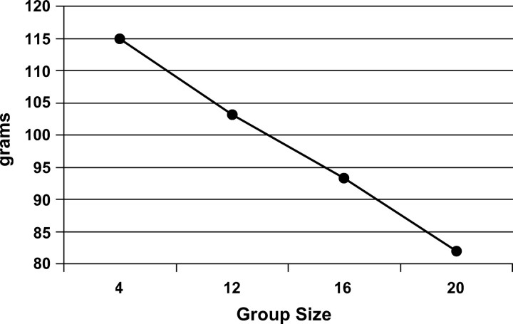
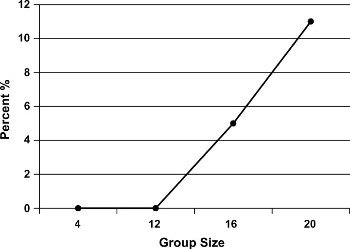
At this level of feed restriction, alternative group sizes were examined such that weight gain was reduced but without excessive mortality being induced. A preliminary experiment was conducted in which five densities were examined: 4, 8, 12, 16, and 20 birds per cage, each replicated six times. Results indicated a linear decline in average weight with increasing number of quail per pen (Figure 6). At 12 birds per cage a 12% decline in average weight occurred with no increase in mortality, but with 16 birds per cage, mortality was 5% (Figure 7). Thus 16 birds per cage was chosen as the optimal group size for this experiment.

Figure 6.—

Mean body weight at 42 days by group (pen) size.

Figure 7.—

Mean percentage of mortality by group size.

The next two generations were devoted to parameter estimation. In each of two rooms, 24 sires were each mated to two dams at random. Females were placed in individual mating cages and a male was placed with each female and was rotated between the two females twice a week. Eggs were marked and collected for 2 weeks and kept in a cooler. After 2 weeks, they were incubated as a group. Upon hatching chicks within a sire family were toe clipped, left or right, to distinguish the dam families, moved to the brooding room, and caged by sire half-sib family. At 2 weeks of age the chicks were wing banded and randomly allocated to grow-out cages, 16 per cage, and up to 12 cages, depending on numbers hatched. If not enough birds were available to fill an additional cage, those extra birds were discarded. At 6 weeks of age, the birds were sexed and weights were recorded. This process was replicated three times. As birds reached 12 weeks of age, random males and females were selected to replace the breeders and data for the second generation were collected.

Selection started after the second generation. For this experiment, a reduced competitive model was used, which, for reasons previously discussed, did not contain the associative environmental effects, Z_A^e. Using these data, REML estimates of genetic parameters were as follows:

The estimated heritability of the associative effects was small and the estimate of the genetic correlation between the direct and associative effects was moderate to large and negative (−0.56). Using these estimates of the genetics parameters, and starting with the adults of the second generation, birds in each room were selected on the basis of solutions from a model that included an index with either direct and associative effects (C-BLUP) or only direct effects (D-BLUP). Within a selection method, sires and dams were kept for breeding until replaced with an animal with a higher breeding value. Selected birds were kept in holding cages for another 4 weeks to become fully sexual mature, i.e., 10 weeks of age, before being used as replacements. Mating was therefore with overlapping generations. Matings between full- and half-sibs were avoided. The experiment was continued for 23 hatches, approximately six generations.

At the termination of the experiment, feed efficiency was measured with the feed restrictors removed. At 2 weeks of age, 60 birds from each line were randomly chosen, weighed, and placed in five cages (12 per cage). Feed was weighed into each trough and birds were allowed to feed continuously. Feed was replaced when the feeders were almost empty. At 6 weeks of age, food was removed 24 hr prior to the birds being weighed. The entire experiment was replicated three times.

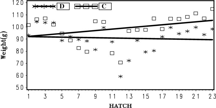
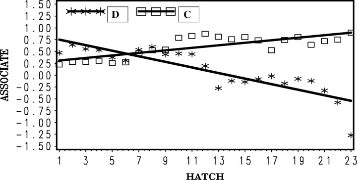
Selection for 6-week body weight was effective for C-BLUP but not D-BLUP (Figure 8). The regression of mean 6-week weight for each hatch on hatch number (b = 0.52 ± 0.25 g/hatch) was significantly (P < 0.05) greater than zero for C-BLUP while negative and not significantly different from zero for D-BLUP (b = −0.10 ± 0.25 g/hatch). The difference between regression coefficients was tested by the interaction of method by hatch and was found to be highly significant (P < 0.006).

Figure 8.—

Mean body weight at 6 weeks for each hatch by method of selection (D-BLUP, selection on direct effects only; C-BLUP, index selection on direct and associative effects).

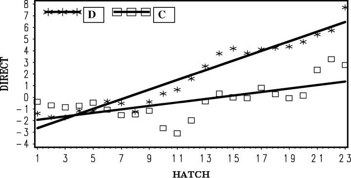
Retrospectively, direct and associative effects were estimated for the birds in the D-BLUP selection experiment using the same model as C-BLUP. The estimated direct and associative effects (Figures 9 and 10) show that the methods differed greatly in what was being selected for. For direct effects, D-BLUP was superior to C-BLUP, which was expected because selection on individual performance in random groups (D-BLUP) places selection pressure only on the direct effects, while with C-BLUP selection was on an index of two components, optimally weighting each.

Figure 9.—

Mean of estimated direct genetic effects for body weight at 6 weeks for each hatch by method of selection (D-BLUP, selection on direct effects only; C-BLUP, index selection on direct and associative effects).

Figure 10.—

Mean of estimated associative genetic effects for body weight at 6 weeks for each hatch by method of selection (D-BLUP, selection on direct effects only; C-BLUP, index selection on direct and associative effects).

Similarly, the methods differed greatly in their impacts on the change in associative effects. The associative effects improved with C-BLUP but became much worse with D-BLUP. This result explains why direct selection on 6-week weight did not produce any response with D-BLUP. The responses in direct and associative effects were in opposite directions, with associative effects negating the positive change in the direct effects. In contrast, with C-BLUP, improvement in associative effects more than compensated for the slower rate of improvement in direct effects, so that, overall, 6-week weight improved.

Mortality was highly variable and the regression of percentage of mortality on hatch number showed a slight reduction in mortality with C-BLUP (b = −0.06 ± 0.15 deaths/hatch) while mortality increased with D-BLUP (b = 0.32 ± 0.15 deaths/hatch). The difference between regression coefficients was tested by the interaction of method by hatch and was found to be significant (P < 0.05). These results are consistent with the above findings that the associative effects were made worse with selection using D-BLUP and better with selection on the index from C-BLUP.

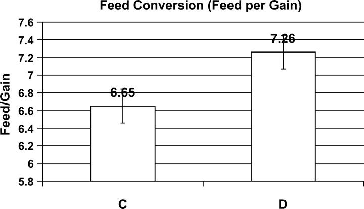
Results from the feed conversion trial at the end of the experiment are given in Figure 11. Both lines of quail wasted enormous amounts of feed, requiring on average 7 grams of feed per gram of gain. Observation of the birds and wastage on the floors showed most of the feed was thrown out in pecking and searching behavior. Nevertheless, the birds selected from the index from C-BLUP had a significantly better efficiency of feed conversion than the D-BLUP-selected birds.

Figure 11.—

Efficiency of feed conversion of quail after 23 cycles of selection with either C-BLUP (index selection on direct and associative effects) or D-BLUP selection on direct effects only.

DISCUSSION

The implications to animals raised in confined spaces are clear. Traditional selection methods using animal model BLUP are detrimental to the well-being of animals if the genetic correlation between direct and associative effects is negative and genetic variability for associative effects is moderate. Because of the biology of most traits, it is difficult to envision a situation in which the genetic correlation between direct and associative effects would be positive. However, not all species may exhibit associative effects. Thus estimation of genetic parameters, including associative effects, is critical before making conclusions about the benefits of alternative selection programs. Results of the computer simulations showed that even if variation due to associative effects is small relative to the environmental variance, the impact of associative effects on group performance can be dramatic, particularly if group size is large. Results of the feed conversion trial confirm the expectation that some associative effects are probably related to food sharing and wastage. An index based on C-BLUP would select for those birds that have lower impacts on other birds and by association would waste less feed. With D-BLUP feed conversion efficiency can be improved only if feed efficiency is included in the selection program.

The importance of competitive effects has long been recognized in plant breeding and forestry applications (see Fasoula and Fasoula 1997 for review) and methods have been proposed to estimate these effects on means and variance (Sakai and Mukaide 1966; Gallais 1976; Wright 1977; Griffing 1989). However, none of those methods have the generality for estimation and prediction for as wide an array of experimental situations as is possible with mixed-model methods. In essence, the method uses genetic and physical measures of distance along with prior estimates of variance components to separate the effects. The relationship matrix provides information that can be used to separate what would normally be confounded effects. In the past the dependence on the relationship matrix for solutions would have rendered the method ineffective in some applications, such as forest tree breeding where open pollination prevents knowledge of both parents. However, with molecular genetic tools, markers can be used to estimate the relationships on the basis of band sharing.

This discussion also highlights a need for more research on optimal experimental designs for estimation of competitive effects. As developed here, individuals were assumed to be somewhat randomly distributed over locations without regard to relationship. Clearly the method will not work if the stand of plants is clonally propagated because the equations will not solve. Alternatively if many varieties are available, each of which is an inbred line, many different designs can be planted in blocks, rows, or randomly. In each of these cases the mixed-model equations will provide solutions, although with different degrees of precision.

Although the method is dependent on prior estimates of variance and covariance components, results from the simulation studies demonstrated that with up to 50% error in parameter estimation the precision with which direct and associative effects were estimated was not appreciably affected, indicating that within the range of effects studied the method is robust. Application of this method in breeding programs will require only that cage, pen number, or location be recorded to define competitors and that mixed-model programs be modified to include associative effects. In this way, selection progress would be enhanced for production traits that are influenced by associate effects while also improving animal well-being, which leads to a win-win situation for the producers, consumers, and animals.

APPENDIX:

SAS CODE TO FIND SOLUTIONS TO EXAMPLE GIVEN IN FIGURE 3

proc iml;

start main;

y={12,

9,

8,

5,

7,

5,

6,

8};

X={1,

1,

1,

1,

1,

1,

1,

1};

G={1 0 0 .5 .5 .5 .5 0 0 0 0,

0 1 0 .5 .5 .5 .5 .5 .5 .5 .5,

0 0 1 0 0 0 0 .5 .5 .5 .5,

.5 .5 0 1 .5 .5 .5 .25 .25 .25 .25,

.5 .5 0 .5 1 .5 .5 .25 .25 .25 .25,

.5 .5 0 .5 .5 1 .5 .25 .25 .25 .25,

.5 .5 0 .5 .5 .5 1 .25 .25 .25 .25,

0 .5 .5 .25 .25 .25 .25 1 .5 .5 .5,

0 .5 .5 .25 .25 .25 .25 .5 1 .5 .5,

0 .5 .5 .25 .25 .25 .25 .5 .5 1 .5,

0 .5 .5 .25 .25 .25 .25 .5 .5 .5 1};

GINV=INV(G);

Z1={0 0 0 1 0 0 0 0 0 0 0,

0 0 0 0 1 0 0 0 0 0 0,

0 0 0 0 0 1 0 0 0 0 0,

0 0 0 0 0 0 1 0 0 0 0,

0 0 0 0 0 0 0 1 0 0 0,

0 0 0 0 0 0 0 0 1 0 0,

0 0 0 0 0 0 0 0 0 1 0,

0 0 0 0 0 0 0 0 0 0 1};

Z2={0 0 0 0 1 0 0 0 1 1 0,

0 0 0 1 0 0 0 0 1 1 0,

0 0 0 0 0 0 1 1 0 0 1,

0 0 0 0 0 1 0 1 0 0 1,

0 0 0 0 0 1 1 0 0 0 1,

0 0 0 1 1 0 0 0 0 1 0,

0 0 0 1 1 0 0 0 0 1 0,

0 0 0 0 0 1 1 1 0 0 0};

Z3={0 1 0 0 0 1 1 0,

1 0 0 0 0 1 1 0,

0 0 0 1 1 0 0 1,

0 0 1 0 1 0 0 1,

0 0 1 1 0 0 0 1,

1 1 0 0 0 0 1 0,

1 1 0 0 0 0 1 0,

0 0 1 1 1 0 0 0};

I8=I(8); *IDENTITY MATRIX;

P={30 −4,

−4 10};

K=inv(P)#60;

K33=60#(1/6);

RHS=(X£*Y)//(Z1£*Y)//(Z2£*Y)//(Z3£*Y);

C=INV (LHS);

BU=C*RHS;

RMSE=(Y£*Y-BU£*RHS)#(1/5);

print BU ;

References

- Campo, J., and P. Tagarro, 1977. Comparison of three selection methods for pupal weight in Tribolium castaneum. Ann. Genet. Sel. Anim. 9 259–268. [DOI] [PMC free article] [PubMed] [Google Scholar]
- Council Directive, 1998 Concerning the protection of animals kept for farming purposes. Council Directive 98/58/EC, Official Journal L 221, 08/08/1998, pp. 0023–0027.
- Council Directive, 1999 Laying down minimum standards for the protection of laying hens. Council Directive 1999/74/EC, Official Journal L 203, 03/08/1999, pp. 0053–0057.
- Craig, D. M., 1982. Group selection vs. individual selection: an experimental analysis. Evolution 36 271–282. [DOI] [PubMed] [Google Scholar]
- Craig, J. V., and W. M. Muir, 1996. Group selection for adaptation to multiple-hen cages: beak-related mortality, feathering and body weight responses. Poult. Sci. 75 294–302. [DOI] [PubMed] [Google Scholar]
- Denison, R. F., E. T. Kiers and S. A. West, 2003. Darwinian agriculture: when can humans find solutions beyond the reach of natural selection. Q. Rev. Biol. 78 145–168. [DOI] [PubMed] [Google Scholar]
- Doolittle, D., S. Wilson and L. Hulbert, 1972. A comparison of multiple trait selection methods in the mouse. J. Hered. 63 366–372. [DOI] [PubMed] [Google Scholar]
- Falconer, D. S., 1981 Introduction to Quantitative Genetics, Ed. 2. Longman, New York.
- Fasoula, D. A., and V. A. Fasoula, 1997. Competitive ability and plant breeding. Plant Breed. Rev. 14 89–138. [Google Scholar]
- Gallais, A., 1976. Effects of competition on means, variances and covariances in quantitative genetics with application to general combining ability. Theor. Appl. Genet. 47 189–195. [DOI] [PubMed] [Google Scholar]
- Garwood, V., and P. Lowe, 1979. Comparison of individual, sire family and index selection for short term rate of egg production in chickens. Poult. Sci. 58 751–753. [Google Scholar]
- Garwood, V. A., and P. Lowe, 1980. An experimental test of the efficiency of family selection in chickens. Theor. Appl. Genet. 56 5–9. [DOI] [PubMed] [Google Scholar]
- Goodnight, C. J., 1985. The influence of environmental variation on group and individual selection in a cress. Evolution 39 545–558. [DOI] [PubMed] [Google Scholar]
- Griffing, B., 1967. Selection in reference to biological groups. I. Individual and group selection applied to populations of unordered groups. Aust. J. Biol. Sci. 10 127–139. [PubMed] [Google Scholar]
- Griffing, B., 1969. Selection in reference to biological groups. IV. Application to selection index theory. Aust. J. Biol. Sci. 22 131–142. [PubMed] [Google Scholar]
- Griffing, B., 1976. a Selection in reference to biological groups. V. Analysis of full-sib groups. Genetics 82 703–722. [DOI] [PMC free article] [PubMed] [Google Scholar]
- Griffing, B., 1976. b Selection in reference to biological groups. VI. Use of extreme forms of nonrandom groups to increase selection efficiency. Genetics 82 723–731. [DOI] [PMC free article] [PubMed] [Google Scholar]
- Griffing, B., 1989. Genetic analysis of plant mixtures. Genetics 122 943–956. [DOI] [PMC free article] [PubMed] [Google Scholar]
- Hamilton, W. D., 1964. The genetic evolution of social behavior. J. Theor. Biol 7 1–16. [DOI] [PubMed] [Google Scholar]
- Henderson, C. R., 1985. Best linear unbiased prediction using relationship matrices derived from selected base-populations. J. Dairy Sci. 68 443–448. [Google Scholar]
- Kestemont, P., S. Jourdan, M. Houbart, C. Melard, M. Paspatis et al., 2003. Size heterogeneity, cannibalism and competition in cultured predatory fish larvae: biotic and abiotic influences. Aquaculture 227 333–356. [Google Scholar]
- Kinney, Jr., T., B. Bohren, J. Craig and P. Lowe, 1970. Responses to individual, family or index selection for short term rate of egg production in chickens. Poult. Sci. 49 1052–1064. [Google Scholar]
- Lynch, M., and B. Walsh, 1998 Genetics and Analysis of Quantitative Traits. Sinauer, Sunderland, MA.
- Maynard-Smith, J., 1976. Group selection. Q. Rev. Biol. 51 277–283. [Google Scholar]
- McCauley, D. E., and M. J Wade, 1980. Group selection: the genotypic and demographic basis for the phenotypic differentiation of small populations of Tribolium castaneum. Evolution 34 83–91. [DOI] [PubMed] [Google Scholar]
- Muir, W. M., 1996. Group selection for adaptation to multiple-hen cages: selection program and direct responses. Poult. Sci. 75 447–458. [DOI] [PubMed] [Google Scholar]
- Muir, W. M., 1997. Genetic selection—strategies for the future. Poult. Sci. 76 1066–1070. [DOI] [PubMed] [Google Scholar]
- Muir, W. M., 2000 The interaction of selection intensity, inbreeding depression, and random genetic drift on short- and long-term response to selection: results using finite locus and finite population size models incorporating directional dominance. Proc. Am. Soc. Anim. Sci. (http://www.asas.org/0602.pdf).
- Perezenciso, M., and M. Toro, 1992. Classical and mixed-model analysis of an index selection experiment for fecundity in Drosophila melanogaster. J. Anim. Sci. 70 2673–2681. [DOI] [PubMed] [Google Scholar]
- Quinton, M., and C. Smith, 1995. Comparison of evaluation-selection systems for maximizing genetic response at the same level of inbreeding. J. Anim. Sci. 73 2208–2212. [DOI] [PubMed] [Google Scholar]
- Sakai, K. I., and H. Mukaide, 1966. Estimation of genetic, environmental, and competitional variances in standing forests. Silvae Genet. 16 149–152. [Google Scholar]
- Sorensen, D. A., and B. W. Kennedy, 1986. Analysis of selection experiments using mixed model methodology. J. Anim. Sci. 63 245–258. [DOI] [PubMed] [Google Scholar]
- Spilke, J., and E. Groeneveld, 1994 Comparison of four multivariate REML (co)variance component estimation packages. Proceedings of the 5th World Congress on Genetics Applied to Livestock Production, Guelph, Ontario, Canada, Vol. 22, pp. 11–14.
- Van Tassell, C. P., and L. D. Van Vleck, 1996. Multiple-trait Gibbs sampler for animal models: flexible programs for Bayesian and likelihood-based (co) variance component inference. J. Anim. Sci. 74 2586–2597. [PubMed] [Google Scholar]
- Wade, M. J., 1976. Group selection among laboratory populations of Tribolium. Proc. Natl. Acad. Sci. USA 73 4604–4607. [DOI] [PMC free article] [PubMed] [Google Scholar]
- Wade, M. J., 1977. An experimental study of group selection. Evolution 31 134–153. [DOI] [PubMed] [Google Scholar]
- Wade, M. J., 1978. A critical review of the models of group selection. Q. Rev. Biol. 53 101–114. [Google Scholar]
- Wade, M. J., and D. E. McCauley, 1980. Group selection: the phenotypic and genotypic differentiation of small populations. Evolution 34 799–812. [DOI] [PubMed] [Google Scholar]
- Wang, C. S., J. J. Rutledge and D. Gianola, 1993. Marginal inferences about variance components in a mixed linear model using Gibbs sampling. Genet. Sel. Evol. 25 41–62. [Google Scholar]
- Williams, G. C., 1966 Adaptations and Natural Selection, pp. 1–14. Princeton University Press/Aldine-Atherton, Princeton, NJ/Chicago.
- Wilson, S. P., 1974. An experimental comparison of individual, family and combination selection. Genetics 76 823–836. [DOI] [PMC free article] [PubMed] [Google Scholar]
- Wilson, D. S., 1983. The group selection controversy and current status. Annu. Rev. Ecol. Syst. 14 159–187. [Google Scholar]
- Wright, A. J., 1977. Predictions of non-linear responses to selection for forage yield under competition. Theor. Appl. Genet. 49 201–207. [DOI] [PubMed] [Google Scholar]
- Wynne-Edwards, V. C., 1986 Evolution Through Group Selection. Blackwell Scientific, Oxford.