Model-based analysis of oligonucleotide arrays: Expression index computation and outlier detection

Abstract

Recent advances in cDNA and oligonucleotide DNA arrays have made it possible to measure the abundance of mRNA transcripts for many genes simultaneously. The analysis of such experiments is nontrivial because of large data size and many levels of variation introduced at different stages of the experiments. The analysis is further complicated by the large differences that may exist among different probes used to interrogate the same gene. However, an attractive feature of high-density oligonucleotide arrays such as those produced by photolithography and inkjet technology is the standardization of chip manufacturing and hybridization process. As a result, probe-specific biases, although significant, are highly reproducible and predictable, and their adverse effect can be reduced by proper modeling and analysis methods. Here, we propose a statistical model for the probe-level data, and develop model-based estimates for gene expression indexes. We also present model-based methods for identifying and handling cross-hybridizing probes and contaminating array regions. Applications of these results will be presented elsewhere.

Oligonucleotide expression array technology (1) has recently been adopted in many areas of biomedical research. As reviewed in ref. 2, 14 to 20 probe pairs are used to interrogate each gene, each probe pair has a Perfect Match (PM) and Mismatch (MM) signal, and the average of the PM–MM differences for all probe pairs in a probe set (called “average difference”) is used as an expression index for the target gene. Researchers rely on the average differences as the starting point for “high-level analysis” such as SOM analysis (3) or two way clustering (4). Besides the original publications by Affymetrix scientists (1, 5), there have been very few studies on important “low-level” analysis issues such as feature extraction, normalization, and computation of expression indexes (6).

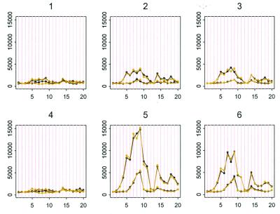
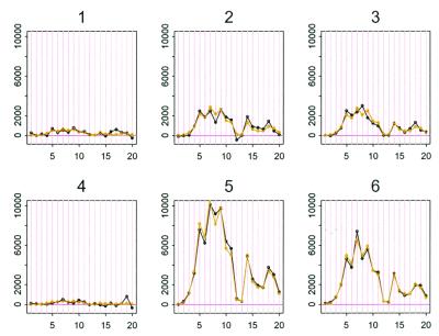
One of the most critical issues is the way probe-specific effects are handled. We have found that even after making use of the control information provide by the MM intensity, the information on expression level provided by the different probes for the same gene are still highly variable. We use a set of 21 HuGeneFL arrays to illustrate our discussion. This data set is typical, in terms of quality and sample size, of a data set from a single-laboratory experiment. We have applied the methodology to many sets of arrays from different laboratories and obtained similar results. Each of these 21 arrays contains more than 250,000 features and 7,129 probe sets. Figs. 1 and 2 show data for one probe set in the first six arrays. This probe set (no. 6,457) will be called probe set A hereafter. There are considerable differences in the expression levels of this gene in the samples being interrogated, as the between-array variation in PM–MM differences is substantial. More noteworthy is the dramatic variation among the PM–MM differences of the 20 probes that interrogate the transcript level. ANOVA of the PM–MM differences of this probe set in these 21 arrays shows that the variation due to probe effects is larger than the variation due to arrays. Specifically, mean squares due to probes and arrays are 38,751,018 and 17,347,098, respectively. This is a general phenomenon: for the majority of the 7,129 probe sets, the rms due to probes is five times or more than that due to arrays. Thus, it is clear that proper treatment of probe effects is an essential component of any approach to the analysis of such expression array data. Below, we introduce a statistical model for the probe-level data to account for probe-specific effects in the computation of expression indexes.

Figure 1.

Black curves are the PM and MM data of gene A in the first six arrays. Light curves are the fitted values to model 1. Probe pairs are labeled 1 to 20 on the horizontal axis.

Figure 2.

Black curves are the PM–MM difference data of gene A in the first six arrays. Light curves are the fitted values to model 2.

In addition, human inspection and manual masking of image artifacts is currently very time consuming and represents a limiting factor in large-scale expression profiling projects. We show that the goodness of fit to our model can be used to construct diagnostics for cross-hybridizing probes, contaminated array regions, and other image artifacts. We use the diagnostics to develop automated procedures for detecting and handling of all these artifacts. This method makes it possible to process and analyze a large number of arrays in a speedy manner.

Statistical Model.

Suppose that a number (I > 1) of samples have been profiled in an experiment. Then, for any given gene, our task is to estimate the abundance level of its transcript in each of the samples. The expression-level estimates are constructed from the 2 × I × 20 (assuming a probe set has 20 probe pairs) intensity values for the PM and MM probes corresponding to this gene. The estimation procedure is based on a model of how the probe intensity values respond to changes of the expression levels of the gene. Let us denote by θ_i an expression index for the gene in the ith sample. We assume that the intensity value of a probe will increase linearly as θ_i increases, but that the rate of increase will be different for different probes. It is also assumed that within the same probe pair, the PM intensity will increase at a higher rate than the MM intensity. We then have the following simple model:

1

Here PM_ij and MM_ij denote the PM and MM intensity values for the ith array and the jth probe pair for this gene, ν_j is the baseline response of the jth probe pair due to nonspecific hybridization, α_j is the rate of increase of the MM response of the jth probe pair, φ_j is the additional rate of increase in the corresponding PM response, and ɛ is a generic symbol for a random error. The rates of increase are assumed to be nonnegative.

We fit model 1 to the 2 × 21 × 20 data matrix for probe set A and Fig. 1 shows the observed and fitted PM and MM intensities for the first six arrays. The model fits the data well. The residual sum of squares is only 1.03% of the sum of squares of the original PM and MM intensities. Thus, this model is able to capture the main relations between the observed intensities for different arrays and probes.

The model for individual probe responses implies an even simpler model for the PM–MM differences:

In the rest of this paper our discussion will be focused on this PM–MM difference model. Feedback from collaborating biologists had indicated that there currently is a strong preference to base all computation directly on the differences between the PM and MM responses in a probe pair. Early experiments using a murine array with a large number of probes (more than 1,000) per gene had shown that the average difference is linear to the true expression level (1). There is also a computational advantage in reducing to differences first, as the fitting of the full data is a more difficult numerical task. Thus, in this first attempt to implement model-based statistical inference, we focus mainly on the analysis of PM–MM differences directly. It should be noted that the MM responses do contain information on the expression index, and that this information can only be recovered by analyzing the PM and MM responses separately.

The foregoing model for the differences is identifiable only if we constrain it in some way. Here we simply make the sum squares of φs to be J (the number of probes):

2

Least square estimates for the parameters are carried out by iteratively fitting the set of θs and φs, regarding the other set as known. For comparison, we also perform least square fitting by using the more standard additive model:

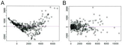
Fig. 3 presents the plots of residuals versus fitted values for these two models. The residuals of the additive model shows a systematic pattern indicating lack of fit. The magnitude of the residual standard deviation of the multiplicative model is much smaller than that of the additive model (1,075 vs. 2,705). The explained energy (R², the ratio of sum of squares of predicted values and sum of squares of original data) is 98.08% and 87.85%, respectively, for the two models. The multiplicative model 2, with 40 parameters, is able to capture the relation among 420 data points (Fig. 2).

Figure 3.

Plots of residuals (y axis) versus fitted value (x axis) for additive model (A) and multiplicative model (B).

Conditional Mean and Standard Error.

Suppose for gene A, the φs have been learned from a large number of arrays, we can then treat them as known constants and analyze the mean and variance of the expression index estimate. For a single array, model 2 becomes:

3

Given the φs, the linear least square estimate for θ is

Hence, an approximate standard error for the least square estimate can be computed:

Similarly, when we regard the estimated θs as fixed, we can calculate standard errors of φs. These standard errors will play an important role in outlier detection and probe selection. We note that the above calculation is conditional in the sense that the φs are regarded as known constants. This is valid if we have a large number of arrays to estimate them accurately, otherwise, the uncertainty in the estimation of these probe-specific parameters must be taken into account in the standard error computation.

Probe selection and Automatic Outlier and Artifact Detection.

Conceptually we can extend expression 2 to model the response of the probe set to all genes in the sample:

4

where θ_i^(k) is the expression level of the kth gene in the ith array, φ_j^(k) is the sensitivity of the jth probe to the kth gene, and n is the total number of different human genes (we do not consider complications such as alternative splicing here). Ideally, we want a probe set to be specific: if a probe set is intended to interrogate gene k, then only the φ_j^(k)s should be nonzero (thus sensitive) and all other φ_j^(k)s should be 0 (thus specific). In this case the observed y_ij are specific signals coming from the target gene and model 4 is reduced to model 2, and the expression indexes θ_i^(k) can be correctly estimated. We note that model 4 is formally a special case of the factor analysis model that is widely used in the social sciences (7).

Although Affymetrix has developed prediction rules to guide the selection of probe sequences with high specificity and sensitivity (1), inevitably there remains some probes hybridizing to one or more nontarget genes. We expect most cross-hybridizing genes to have expression patterns (in a large set of samples) different from that of the target gene, and different probes in a probe set to cross-hybridize to different nontarget genes. For a nontarget interfering gene k′, the sensitivity indexes φ_j^(k′) are expected to be small except for one or two probes in the probe set. The mixed response of a probe set to target and nontarget genes suggests that probe selection (in the analysis stage) may enhance the specificity in estimating the expression levels of the target gene θ_i^(k).

In the standard analysis (5), the mean and standard deviation of the PM–MM differences of a probe set in one array are computed after excluding the maximum and the minimum. If a difference deviates by more than 3 SD from the mean, a probe pair is marked as an outlier in this array and discarded in calculating average differences of both the baseline and the experiment arrays. One drawback to this approach is that a probe with a large response might well be the most informative but may be consistently discarded. Furthermore, if we want to compare many arrays at the same time, this method tends to exclude too many probes.

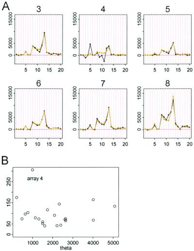
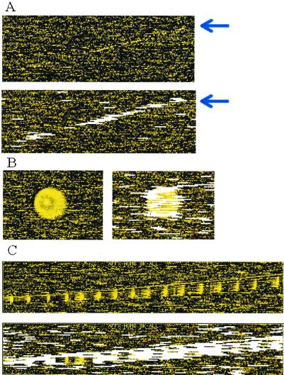
We exploit our model to detect and handle cross-hybridizing probes, image contamination, and outliers from other causes. For a particular probe set, its 20 φ values constitute its “probe response pattern,” and the model hypothesizes that the 20 differences in an array should follow this pattern and are scaled by the target gene's expression index (θ) in this array. The (conditional) standard error attached to a fitted θ is a good measure of how the 20 differences in the corresponding array conform to the probe response pattern. For example, in Fig. 4B, array 4 is identified as an “outlier array” because the estimated θ₄ has a large standard error. Close examination of Fig. 4A reveals that the probe responses in array 4 deviates from the consistent patterns shown in the other arrays. This could be due to various reasons including image artifacts (Fig. 5). The probe responses in this array will distort the fitting of the probe response pattern. To guard against this, we exclude outlier arrays (identified by large standard errors) and use the remaining arrays to estimate the probe response pattern. For an outlier array, we still compute its expression index conditional on the estimated probe response pattern, with the attached large standard error indicating poor reliability of this expression index.

Figure 4.

(A) Six arrays of probe set 1,248. (B) Plot of standard error (SE, y axis) vs. θ. The probe pattern (black curve) of array 4 is inconsistent with other arrays, leading to unsatisfactory fitted curve (light) and large standard errors of θ₄.

Figure 5.

(A) A long scratch contamination (indicated by arrow) is alleviated by automatic outlier exclusion along this scratch. (B and C) Regional clustering of array outliers (white bars) indicates contaminated regions in the original images. These outliers are automatically detected and accommodated in the analysis. Note that some probe sets in the contaminated region are not marked as array outliers, because contamination contributed additively to PM and MM in a similar magnitude and thus cancel in the PM–MM differences, preserving the correct signals and probe patterns.

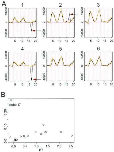
In model 2 the role of θ and φ are symmetric. Therefore, we can use the conditional standard errors of the estimated φ_js to identify problematic probes. In Fig. 6, probe 17 (indicated by arrow in several arrays) has peculiar behavior that is inconsistent with the rise and fall of other probes. This inconsistency is probably due to the cross-hybridization of this probe to nontarget genes. Fig. 6B shows that this nonspecific probe can be identified by the large standard error associated with φ₁₇. Finally, we must also consider a “single outlier” which might be an image spike in one array affecting just one PM–MM difference. Such a single outlier (say d_ij in the data matrix) may affect estimates of both θ_i and φ_j and we can identify it by the large residual for this data point. Once identified, single outliers are regarded as “missing data” in the model fitting.

Figure 6.

(A) Probe 17 of probe set 1,222 is not concordant with other probes (black arrows) and is numerically identified by the outstanding standard error of φ₁₇ (B).

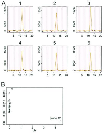
Besides array, probe, and single outliers, there are several other undesirable artifacts in the data that we wish to handle. Fig. 7A shows a responsive probe 12 amidst other nonresponsive probes. Generally, if the target gene exists in the samples, we expect more than one probe of 20 to respond at various levels. In this case it is most likely that the target gene is not present in any samples, and that the large response by probe 12 is due to cross-hybridization to nontarget genes. Although the model fits well in this case (99.83% variance explained), it is prudent to exclude this probe because of its unusually high leverage. Fig. 7B shows that such a probe can be automatically identified through its large φ value. If it contributes more than 80% to the sum of squares of the φ_js in the probe set, we classify a probe as “high-leverage” and exclude it during the fitting of the model. A similar procedure is used to identify high leverage arrays.

Figure 7.

(A) Probe set 3,562 has a single high-leverage probe 12, and the fitted light curves almost coincide with the black data curve. (B) φ₁₂ is large compared with other φs close-to-zero value. Note that Affymetrix's superscoring method works here by consistently excluding this probe.

To implement the above ideas, we iteratively identify array, probe, and single outliers. Specifically, we first fit the model to the data table of one probe set, identifying θs (arrays) with large standard error (more than three times as large as the median standard error of all θs) or dominating magnitude (θ in 2 is more than 80% of the sum of squares of all θs), and mark these arrays as array outliers. Next, with these array outliers excluded, we work on a data table with fewer rows (discarding outlier arrays), and fit the model again. This time we inspect the standard errors and magnitudes of φs, in the hope of excluding probe outliers. If a φ has a negative value, we also regard it as probe outlier and exclude the corresponding probe. In effect, the data table shrinks in columns and we fit the model again to this new data table. Note that, although some arrays and probes may not be used in fitting the model, we still can regress the data in one array (excluding probes not used in model fitting) against the estimated probe pattern (φs) to get an estimate of the expression levels (θs) of the excluded arrays. After probe outliers are excluded, we evaluate all arrays for outliers again and compare them to the set of array outliers in the previous round to see if there is any change. This procedure is repeated until the set of probe and array outliers does not change anymore. (In some cases, they may cycle in a small number of slightly different sets.) Along the iteration we will also identify some single data point outliers with large residuals and mark them as missing data when fitting the model. In general, 5–10 iterations will lead to a converged set of outliers.

Results

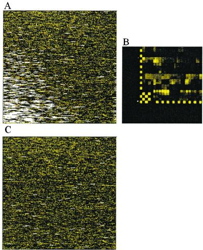
We apply this model-based analysis to all 7,129 probe sets of the HuGeneFL arrays. Fig. 8 shows excluded array and single outliers for two arrays. As we have seen from Fig. 5, image contamination can be handled automatically by reasonably marking array and single outliers and excluding them from model fitting. Such contamination would lead to incorrect expression, and fold change calculation if left unattended in the data. There are arrays with a large number of array and single outliers (Fig. 8B). Presumably, such arrays underwent severe sample contamination which destroyed the probe pattern of many probe sets and introduced many single outliers. Again the model automatically excludes the array from model fitting to avoid the influence of these bad arrays on good arrays and attaches large standard errors to the expression indexes of contaminated probe sets. Fig. 9 shows a case where the output by the genechip software (Affymetrix, Santa Clara, CA) is presumably incorrect, most probably because of a misaligned corner. This is detected by an unusually large number of array and single outliers near the corner. We also intentionally include a murine MU11KSUBA array with the 21 human arrays to assess its effect on the analysis. This has little effect on the outlier image of the human arrays, but more than two-thirds of “probe sets” on the murine array are detected as outliers (Fig. 10). For the remaining “probe sets,” their signals on the murine array are mostly close to zero. These are not detected as outliers as they can fit the human probe patterns (φs) by taking low θ values, but they will not bias the estimation of the probe response patterns of the human arrays.

Figure 8.

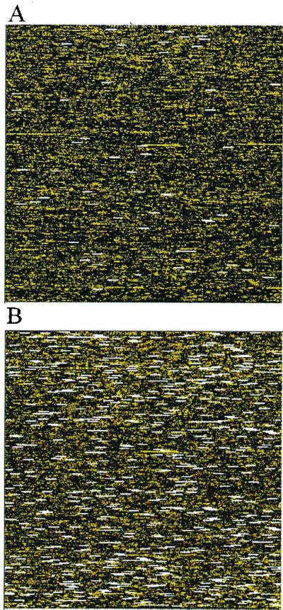
(A) A typical array (array 5) with array outliers (white bars) and single outliers (red dots) marked. (B) Array 4 has an unusually large number of array and single outliers, indicative of possible sample contamination.

Figure 9.

(A) Array 9 initially has an unusually large number of array and single outliers in the lower-left region. (B) The lower-left corner pixel position (white dot) appears to be off by about one feature and therefore leads to incorrect gridding and averaging of many features in the lower-left region. This is hard to detect by visual inspection of the original image. (C) After manually setting the correct corner pixel position, the array is salvaged.

Figure 10.

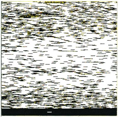
The outlier image of an intentionally misplaced murine array in a set of human arrays (4,647 array outliers and 905 single outliers detected).

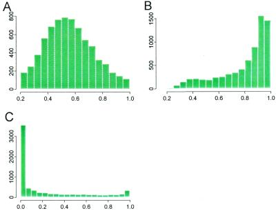
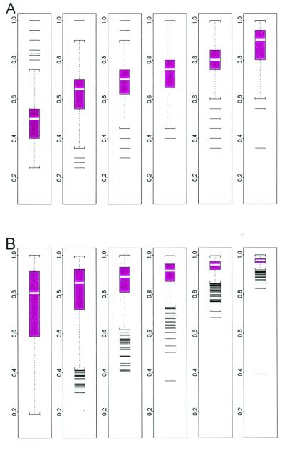
Fig. 11A shows that for 60.2% of the probe sets, we use more than half of the probes to fit the model. Fig. 11B shows that the explained energy is high (R² greater than 80%) for 63.3% of the probe sets. To investigate the reason for the low probe usage and poor R² for some probe sets, we examine the relationship between probe usage, explained energy, and the presence percentage (percentage of arrays where a probe set is called “present” by genechip; Fig. 11C). Fig. 12A shows that high presence percentage usually leads to high probe usage. Fig. 12B demonstrates that when a gene is present in many arrays, the explained energy of the corresponding probe set tends to be high. Clearly, when a gene is absent in most arrays, the variations in the observed data are mostly due to the noise term and one should not expect the model to explain a large fraction of this variation. In this case, there is not much information in the data to determine the φs, but the θs are still correctly estimated to be close to zero.

Figure 11.

Histograms of percent of probe used (A), explained energy (B), and presence percentage (C) for all 7,129 probe sets. As seen from C most genes are only present in a few arrays.

Figure 12.

Boxplots of probe usage (A) and explained energy (B) stratified by presence percentage (the number of presences of a gene in 21 arrays and the subpopulation size for the 6 boxplots are: 0–3, 4,365; 4–7, 817; 8–11, 567; 12–15, 520; 16–19, 518; and 20–21, 342). When presence percentage is high, the excluded probes tend to be cross-hybridizing probes; when presence percentage is low, PM–MM differences fluctuating around 0 may result in many negative probes and exclusion of them. As more arrays enter the database, we may reuse these probes if they respond positively to target expressions. The more arrays in which a target gene is present, the better the explained energy.

Conclusions

We have proposed a statistical model for oligonucleotide expression array data at the probe level. Based on this model, we are able to address several important analysis issues that are difficult to handle by using current approaches. These include accounting for individual probe-specific effects, and automatic detection and handling of outliers and image artifacts. Computer programs implementing these methods are available on request for nonprofit research. In a follow-up paper, we will discuss the computation of standard errors (SE) for expression indexes and confidence intervals (CI) for fold changes, how the availability of the SE and CI values impact downstream analysis, and metaanalysis of pooled data from different experiments.

Abbreviations

PM

perfect match

MM

mismatch

References

- 1.Lockhart D, Dong H, Byrne M, Follettie M, Gallo M, Chee M, Mittmann M, Wang C, Kobayashi M, Horton H, et al. Nat Biotechnol. 1996;14:1675–1680. doi: 10.1038/nbt1296-1675. [DOI] [PubMed] [Google Scholar]
- 2.Lipshutz R J, Fodor S, Gingeras T, Lockhart D. Nat Genet, supplement. 1999;21:20–24. doi: 10.1038/4447. [DOI] [PubMed] [Google Scholar]
- 3.Tamayo P, Slonim D, Mesirov J, Zhu Q, Kitareewan S, Dmitrovsky E, Lander E S, Golub T R. Proc Natl Acad Sci USA. 1999;96:2907–2912. doi: 10.1073/pnas.96.6.2907. [DOI] [PMC free article] [PubMed] [Google Scholar]
- 4.Alon U, Barkai N, Notterman D A, Gish K, Ybarra S, Mack D, Levine A J. Proc Natl Acad Sci USA. 1999;96:6745–6750. doi: 10.1073/pnas.96.12.6745. [DOI] [PMC free article] [PubMed] [Google Scholar]
- 5.Wodicka L, Dong H, Mittmann M, Ho M, Lockhart D. Nat Biotechnol. 1997;15:1359–1367. doi: 10.1038/nbt1297-1359. [DOI] [PubMed] [Google Scholar]
- 6.Schadt E, Li C, Su C, Wong W H. J Cell Biochem. 2001;80:192–202. [PubMed] [Google Scholar]
- 7.Press J. Applied Multivariate Analysis. Rinehart and Winston, New York: Holt; 1972. [Google Scholar]