Noise in a Small Genetic Circuit that Undergoes Bifurcation

Abstract

Based on the consideration of Boolean dynamics, it has been hypothesized that cell types may correspond to alternative attractors of a gene regulatory network. Recent stochastic Boolean network analysis, however, raised the important question concerning the stability of such attractors. In this paper a detailed numerical analysis is performed within the framework of Langevin dynamics. While the present results confirm that the noise is indeed an important dynamical element, the cell type as represented by attractors can still be a viable hypothesis. It is found that the stability of an attractor depends on the strength of noise related to the distance of the system to the bifurcation point and it can be exponentially stable depending on biological parameters.

INTRODUCTION

We have entered the post genomic era. The human genome has been sequenced as have a number of other organisms. We are now confronted with the problem of understanding the behavior of simple and complex genetic regulatory networks. For example, the human genome has between 20,000 and 25,000 genes whose activities are coordinated by a regulatory network of their products. As such, the genome is a parallel processing nonlinear dynamical system. For a number of decades, this system has been modeled by a variety of approaches, ranging from random Boolean networks introduced by [1], to differential equations [2], and piecewise linear differential equations [3]. Such nonlinear dynamical systems typically have state spaces with dynamical trajectories that each flow to an attractor, which might be a steady state, limit cycle, quasi-periodic orbit, or strange attractor. Because, even in the binary idealization of Boolean nets, a genome with 25,000 genes has states, and a human has only about 265 cell types [4], it is obvious that not all states of gene activities can correspond to cell types. A plausible hypothesis is that cell types correspond to alternative attractors of the network [5].

At present, no data support or refute the hypothesis that cell types correspond to alternative attractors. However, Aldana et al. [6] have made the important criticism with respect to Boolean networks that noise may render such attractors a poor model of cell types because closure of an attractor (a state cycle) in the discrete dynamics is delicate. This is an important criticism.

In response to this concern we have, first, noted that metaplasias in organisms may in fact be a response to such noise [5] and here undertake a study of a very simple bistable model genetic circuit comprised of continuous variables. The move to continuous variables creates a continuous state space. Here the two alternative stable steady states of the system each lie in a continuous valued basin of attraction, such that small noise will leave the system in the same basin. Our model contains a parameter which, when tuned, causes the system to bifurcate such that it loses its lower stable steady state.

We utilize Langevin equations [7] to model noise in this simple system and study mean escape times as a function of the noise level and a bifurcation parameter Z. Our results show that escape from an attractor is exponentially distributed in time, but can be made very long for small noise. In addition, we study the occupancy distribution for this noisy small circuit and show for a range of parameter values that the system remains in the vicinity of the steady states. Overall, our results suggest that noise is an important issue, that attractors remain attractive dynamical objects to constitute cell types in the presence of small amounts of noise and implies the possibility that network motifs [8-10] may have evolved to dampen such noise.

THE MODEL GENETIC CIRCUIT

The equations for our model were based on a Boolean function of three variables, where Y responded to inputs received from X or from Z and X responded directly to Y. The system of differential equations was as follows:

$$\frac{dx}{dt}=\frac{y^2}{{(y+1)}^2}-K_{1}x\frac{dy}{dt}=\frac{{(x+z)}^2}{{((x+z)+1)}^2}-K_{2}y$$

In these equations, we treat Z as an exogenous parameter that is varied in our numerical experiments. To determine the steady states of the system the null clines were plotted. There are three steady states in our model: a lower stable steady state, an unstable steady state slightly above the lower one, and an upper steady state well above the unstable steady state. The lower and upper steady states are separated by a separatrix that travels through the unstable steady state. The separatrix divides the x-y state space into two basins of attraction. Trajectories above and below the separatrix flow to the upper and lower stable steady state respectively. The separatrix itself is a manifold of dimension 1 where trajectories flow to the unstable steady state (Figure 1).

FIGURE 1.

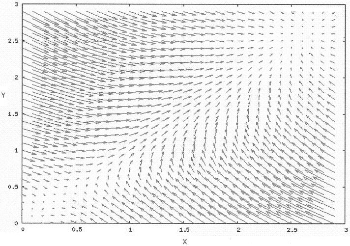
Plot of the vector field for the deterministic equation. There are three steady states. A lower stable steady state at the origin, an upper steady state around x = 2.5 and y = 2.5 and an unstable steady state around x = 0.25 and y = 0.25.

This system of equations also has the property that as Z increases the steady states bifurcate. At Z = 0 the lower steady state is at the origin but as Z increases the lower steady state moves up toward the unstable steady state, which moves simultaneously towards the lower stable steady state. Eventually the two states merge and disappear leaving only the stable upper steady state and the whole system bifurcates.

In order to study the effects of noise on our system we used a Langevin equation where a noise term was added to the end of each of the equations. For each variable, x and y, the additive noise term was governed by a Gaussian distribution with a variance equal to the absolute value of the sum of the two terms in the deterministic differential equation for that variable. The variance equation was developed using the work of van Kampen [7] on the diffusion approximation. The scale of the noise term was controlled by the use of a constant multiplicative factor, λ, which served to increase or decrease the variance of the noise. Thus, the equations are:

$$\begin{array}{cc}\hfill \frac{dx}{dt}=\left(\frac{y^2}{{(y+1)}^2}-K_{1}x\right)& +\lambda \hfill \\ \hfill & \frac{dy}{dt}=\left(\frac{{(x+z)}^2}{{((x+z)+1)}^2}-K_{2}y\right)+\lambda \hfill \end{array}$$

where λ respectively equals:

$$\begin{array}{cc}\hfill \lambda =\gamma \mid \frac{y^2}{{(y+1)}^2}+K_{1}x\mid & \hfill \\ \hfill & \lambda =\gamma \mid \frac{{(x+z)}^2}{{((x+z)+1)}^2}+K_{2}y\mid \hfill \end{array}$$

To simulate the noise we sampled values from a Gaussian distribution with a mean of zero. We note that the use of a Langevin equation to model noise in real genetic circuits is a very crude approximation. To be realistic one would need to model molecular noise at each step in the transcription, translation and gene regulation process. Our aim is not detailed realism but to obtain a qualitative view of the effects of noise on a small, bifurcating, genetic circuit model.

MATERIALS AND METHODS

The system of equations was solved algorithmically using the 4th-order Runge-Kutta method. The Gaussian distribution was sampled by the use of the Box-Muller method [11].

The addition of a noise term to our system of equations presented the problem that values could now go negative. Because negative values have no counter point in biological reality we needed to set boundary conditions to avoid them. The variance equation prevented negative values close to the origin since the variance goes to zero but negative values were possible along the axes away from the origin. Our chosen method was to throw out noise that produced negative values and resample until we stayed within bounds. This was an effective solution because for most conditions negative values were rare. But under certain conditions discussed later it did create a positive bias in the noise and compounded some problems that created meaningless numerical data under some circumstances.

In order to determine how stable the upper and lower steady states were in the presence of noise the first question we asked is under what conditions do trajectories released at or near one steady state move across the separatrix. More precisely, as a function of the noise level, λ, and Z, what is the distribution of these first passage trajectories from one basin of attraction across the separatrix into the other basin.

In order to study this question it was necessary to determine the location of the separatrix itself. Thus the first step was to determine the function that described the sepratrix. We did this by selecting a point on each axis and then determining if a trajectory starting at that point was above or below the sepratrix. We would then select a point either larger or smaller on the axis and check again. We sampled points above and below the sepratrix moving points closer to each other each time until we could no longer calculate whether we were above it or below the separatrix. We determined that this was where trajectories leaving those infinitesimal neighborhoods of each axis flowed along the separatrix to the unstable steady state. To do so, we followed the deterministic vectors from each axis. The vector magnitudes approached zero at the unstable steady state so the system was on a trajectory extremely close to the true separatrix. The vectors' directions relative to each other and the unstable steady state approximated a straight line. We then calculated the line equation that best approximated the separatrix.

To determine the distribution of first passage times for each value of λ, the scale of the noise, and each value of Z, the algorithm was run with noise. We carried out 1000 runs for each value of λ and Z and initial state studied. Each run was carried forward for 1000 time steps or until we detected that the system had crossed the line equation approximating the sepratrix. We outputted the time iteration at which this occurred as the first passage time. Thus, we generated a distribution of first passage times for crossing the separatrix.

We used a range of λ values from 0.5 to 5.0 with increments of 0.5 for each run. We also examined the effects of Z by starting with Z = 0 and increasing it by 0.01 until we reached the bifurcation value of around Z = 0.16. The initial values for x and y are necessary for the Runge-Kutta method. For Z values greater than zero we used the stable steady state calculated using the null clines as the initial conditions. For Z = 0 though the steady state was at the origin and no noise would be present. So we used a range of initial conditions between the origin and the separatrix.

We next examined the occupancy grid generated by running the simulation for a set number of points around each of the stable steady states. To generate the occupancy grid we ran the program for 10,000 time steps 1,000 times for a total of 10,000,000 points. We did this rather than just using 10,000,000 time steps so the noise variance would be reset regularly making sure the system did not become trapped around the origin. Visualization for 10,000,000 points became difficult so a random sample of 500,000 points was drawn from each run and was used for graphing.

The Z values for both steady states were selected the same way as for the first passage time. We started with Z = 0 and increased it by 0.01 until we reached the bifurcation value of around Z = 0.16. The λ for the lower steady state ranged from 0.5 to 5.0 in increments of 0.5. The upper steady state required lower values of noise to achieve meaningful data, so the λ values ranged from 0.1 to 1.0 in increments of 0.1.

RESULTS

The first data we gathered were the vector field for the deterministic equations showing the lower steady state, the separatrix, and the upper steady state. The vector fields were generated for a range of increasing Z values showing the lower steady state moving up toward the separatrix till they merge and the system is left with only the upper steady state (Figures 2 and 3). This is the bifurcation point and was calculated to occur at approximately Z = 0.16.

FIGURE 2.

(A) A probability plot for the exponential distribution (Z = 0.5, γ = 1.0). The fact that most points lie on a straight line indicates that they are exponentially distributed.

FIGURE 3.

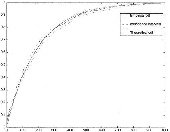
(B) The empirical and theoretical maximum likelihood estimated cumulative distribution functions for Z = 0.5 and λ = 1.0. Lower and upper confidence bounds are shown.

The mean escape times for the lower steady state proved to be exponentially distributed under the Gaussian noise model. A probability plot for the exponential distribution, shown in Figure 2, provides evidence for this assertion. The values Z = 0.5 and λ = 1.0 were used. Ideally, if the data do come from an exponential distribution (with some unknown parameter), all data points should lie on a straight line. The superimposed straight line (dashed) is the robust linear fit of the sample order statistics corresponding to the first and third quartiles. Note that the fit is quite good and the deviation only begins to occur after probability of approximately 0.99, which is in the tail of the distribution. This fact is hardly surprising, because it corresponds to data with a very low probability of occurrence (i.e., very large escape times). Indeed, similar deviations in the tail of the distribution would occur with pseudorandom numbers generated from an exponential distribution.

As further validation, we computed the maximum likelihood estimate of the parameter, μ, of the exponential distribution and plotted the cumulative distribution function (cdf) with this parameter together with the empirical cdf generated from the data. Figure 3 illustrates this for Z = 0.5 and λ = 1.0. Additionally, lower and upper confidence bounds for the empirical cdf, calculated using Greenwood's formula [12], are shown with dashed lines. Visual inspection strongly suggests that the exponential distribution provides the correct fit to the data.

An interesting result that we found for Z = 0, where the lower steady state was at the origin, was escape across the separatrix had to occur early in the run. If escape did not occur early it did not occur at all. We interpret this as a consequence of the fact that as the system follows trajectories of the deterministic system towards the lower steady state at the origin, the noise term's variance goes to 0. Hence, once very close to the origin, escape does not occur.

The system of equations bifurcates as Z increases to approximately 0.16. As Z increased and the lower steady state moved toward the separatrix, the mean escape time for each value of λ decreased. Figure 4 shows the distribution of exponential escape time values as a function of λ and Z. Larger values of λ produced smaller mean escape times for the noise. Similarly, larger Z produced smaller mean escape times.

FIGURE 4.

Graph of the mean escape times, μ, as a function of Z and λ. As λ increases the escape times become smaller. As Z approaches the bifurcation the escape times also decrease. For Z = 0 each of the initial conditions is shown. For all conditions of Z = 0 the system either escaped early or did not escape at all so there was little change in escape time as λ changed.

The upper steady state presented several problems. The positive bias in the boundary conditions became important at this point. The distance needed to travel from the upper steady state across the separatrix is several magnitudes greater than from the lower steady state to the separatrix. The noise, therefore, must also be several times greater in magnitude to create any significant passage. Noise that is large enough to cause passages across the separatrix at this level is also large enough to cause the system to go into the negative range of values. Our approach to dealing with negative values was to toss them out and regenerate noise until we got a positive value. Because negative noise values had a significant chance of crossing the axis, resulting in negative values, we discarded a lot of negative noise. Positive noise, though, can not cross the axis. Therefore, we discarded large amounts of negative noise and kept all positive noise. This creates a bias for positive noise that pushes the values of the system beyond anything that is meaningful. When we bring the noise value low enough so we do not have to throw out values then there is not enough noise to create any significant number of passage times across the separatrix.

The occupancy grids for both the upper and lower steady state showed little deviation around the steady state for a small enough range of noise. The upper steady state also showed stability for noise values about a tenth of the size used for the lower steady state. Occupancy was also calculated for 10,000,000 time steps. Because the 10,000,000 point files were to large for visualization we randomly selected 10,000 points and used them to construct graphs. Figure 5 shows such a graph and that for smaller ranges of noises escapes did not occur even over very long time periods.

FIGURE 5.

Plot of 10,000 time steps in an occupancy grid around the lower steady state. This graph shows that even in the presence of noise the system can stay very close to the steady state.

DISCUSSION

We have carried out simulations of a simple bistable model genetic network in the presence of noise, modeled as additive Gaussian noise. The circuit undergoes a bifurcation as an exogenous input, Z, is increased from 0.0 to approximately 0.16. As the bifurcation is approached, the lower stable steady state approaches the unstable steady state lying on the separatrix. Our initial conditions were either the lower steady state for Z > 0, or a set points at increasing distances from the lower steady state at the origin for Z = 0. As expected, using Gaussian noise, the first passage time across the separatrix was exponentially distributed. As shown in Figure 5, in general, increasing noise, λ, and increasing Z before bifurcation led to shorter mean escape times. It is important to note that the infinite-tailed Gaussian of the standard Langevin equation is not established as a good model of the detailed noise fluctuations concerning actual transcription, translation, and product life times. In real cells, the numbers of molecules is low and may require another detailed noise model.

Our purpose in utilizing the standard Langevin equation was to begin to gain some insight into the effects of noise on bistable model genetic circuits. The main results show that, for low enough noise, the system remains in the vicinity of the lower or upper steady state for very long times. Our efforts are a response to a criticism of random Boolean network models of gene networks by Aldana et al. [6], who point out that a small fraction of single gene “flips” move the system from one attractor to another, hence that attractors are unstable to noise. The use of stochastic differential equations here yields two steady states with continuous, finite sized basins of attraction around each stable steady state. In this context, attractors remain a viable model of cell types: With small enough noise the system remains near the initial steady state for arbitrarily long times. At the biological level, we do not know if real cells rarely change to new cell types, although the phenomenon of metaplasias may reflect such transitions. We should point out that in a related genetic circuit the full range of stability has been absorbed in vivo experimentally and modeled mathematically [13].

Only future work will establish whether real cell types correspond to attractors and the extent of perturbation by noise and possible rare transitions to other cell types induced by endogenous noise. In the meantime, the hypothesis that attractors correspond to cell types in the presence of some low amount of noise appears justified.

REFERENCES

- 1.Kauffman SA. Metabolic stability and epigenesis in randomly constructed genetic nets. J Theor Biol. 1969;22:437–467. doi: 10.1016/0022-5193(69)90015-0. [DOI] [PubMed] [Google Scholar]
- 2.Mestl T, Plahte E, Omholt SW. A mathematical framework for describing and analysing gene regulatory networks. J Theor Biol. 1995;176(2):291–300. doi: 10.1006/jtbi.1995.0199. [DOI] [PubMed] [Google Scholar]
- 3.Glass L. Classification of biological networks by their qualitative dynamics. J Theor Biol. 1975;54:85–107. doi: 10.1016/s0022-5193(75)80056-7. [DOI] [PubMed] [Google Scholar]
- 4.Alberts B, Johnson A, Lewis J, Raff M, Roberts K, Walter P. Molecular Biology of the Cell. 4th Garland Science; New York, NY: 2002. [Google Scholar]
- 5.Kauffman SA. The Origins of Order: Self-organization and Selection in Evolution. Oxford University Press; New York: 1993. [Google Scholar]
- 6.Aldana M, Coppersmith S, Kadanoff LP. Boolean dynamics with random couplings. In: Kaplan E, Marsden JE, Sreenivasan KR, editors. Perspectives and Problems in Nonlinear Science. 2003. pp. 23–89. Boolean Dynamics with Random Couplings; Springer Applied Mathematical Sciences Series. [Google Scholar]
- 7.Van Kampen NG. Stochastic Processes in Physics and Chemistry. Elsevier Science. 2001 [Google Scholar]
- 8.Milo R, Shen-Orr S, Itzkovitz S, Kashtan N, Chklovskii D, Alon U. Network motifs: Simple building blocks of complex networks. Science. 2002;298:824–827. doi: 10.1126/science.298.5594.824. [DOI] [PubMed] [Google Scholar]
- 9.Mangan S, Alon U. Structure and function of the feed-forward loop network motif. Proc Natl Acad Sci USA. 2003;100:11980–11985. doi: 10.1073/pnas.2133841100. [DOI] [PMC free article] [PubMed] [Google Scholar]
- 10.Dobrin R, Beg QK, Barabasi AL, Oltvai ZN. Aggregation of topological motifs in the Escherichia coli transcriptional regulatory network. BMC Bioinformatics. 2004;30(1):10. doi: 10.1186/1471-2105-5-10. [DOI] [PMC free article] [PubMed] [Google Scholar]
- 11.Ross SM. A First Course in Probability. 5th Prentice Hall; 1997. [Google Scholar]
- 12.Armitage P, Berry G. In: Survival analysis. In: Statistical Methods in Medical Research. 3d Armitage P, Berry G, editors. Blackwell Scientific Publications; Oxford: 1994. pp. 469–492. [Google Scholar]
- 13.Zhu X-M, Yin L, Hood L, Ao P. Robustness, stability and efficiency of phage lambda genetic switch: dynamical structure analysis. J Bioinf Comput Biology. 2005;2:785–817. doi: 10.1142/s0219720004000946. [DOI] [PubMed] [Google Scholar]