Selection for Recombination in Structured Populations

Abstract

In finite populations, linkage disequilibria generated by the interaction of drift and directional selection (Hill-Robertson effect) can select for sex and recombination, even in the absence of epistasis. Previous models of this process predict very little advantage to recombination in large panmictic populations. In this article we demonstrate that substantial levels of linkage disequilibria can accumulate by drift in the presence of selection in populations of any size, provided that the population is subdivided. We quantify (i) the linkage disequilibrium produced by the interaction of drift and selection during the selective sweep of beneficial alleles at two loci in a subdivided population and (ii) the selection for recombination generated by these disequilibria. We show that, in a population subdivided into n demes of large size N, both the disequilibrium and the selection for recombination are equivalent to that expected in a single population of a size intermediate between the size of each deme (N) and the total size (nN), depending on the rate of migration among demes, m. We also show by simulations that, with small demes, the selection for recombination is stronger than both that expected in an unstructured population (m = 1 − 1/n) and that expected in a set of isolated demes (m = 0). Indeed, migration maintains polymorphisms that would otherwise be lost rapidly from small demes, while population structure maintains enough local stochasticity to generate linkage disequilibria. These effects are also strong enough to overcome the twofold cost of sex under strong selection when sex is initially rare. Overall, our results show that the stochastic theories of the evolution of sex apply to a much broader range of conditions than previously expected.

WHY sex and recombination are so widespread in nature is an age-old debate in evolutionary biology. While some theories invoke mechanistic advantages for sex (e.g., DNA repair), most theories account for sex on the basis of its effects on multilocus allelic combinations (Kondrashov 1993). These hypotheses can be termed generative hypotheses, because they focus on the effects of sex and recombination on the array of genotypes generated within a population. According to several generative hypotheses, sex and recombination are advantageous because they facilitate the response to selection by reducing negative linkage disequilibria, whereby beneficial alleles are found on low-fitness genetic backgrounds, thereby increasing the genetic variance in fitness (Maynard Smith 1971; Felsenstein 1974). This class of explanations is consistent with experiments showing that higher rates of recombination often evolve as a pleiotropic response to artificial selection for other traits (see Otto and Barton 2001 for a review).

Generative hypotheses can be classified according to the force generating linkage disequilibria (LD) within a population (Kondrashov 1993; Barton 1995a; Otto and Lenormand 2002). LD can be produced by selection involving epistasis (Feldman et al. 1980) or can result from the interaction of drift with directional selection (Hill and Robertson 1966). In this article we focus on drift-based explanations for LD. Because drift in the presence of selection causes an accumulation of negative linkage disequilibria, linkage imposes a limit on the efficacy of natural selection in finite populations (Hill and Robertson 1966; Felsenstein 1974; Barton 1995b). Sex and recombination release populations from this limit, by allowing beneficial alleles within different individuals to come together, as recognized early on by both Fisher (1930) and Muller (1932). The accumulation of negative disequilibria due to drift in the presence of selection on linked loci is often referred to as the Hill-Robertson effect (HRE). The HRE results in selective interference among loci, which reduces the probability of fixation of beneficial alleles as the population size gets smaller or as linkage among loci tightens (Hill and Robertson 1966; Barton 1995b). In the extreme case of an asexual population, the HRE affects the entire genome and is then referred to as “clonal interference” (Gerrish and Lenski 1998).

The HRE imposes an important limit on the response to selection on linked sets of loci in sexual species and on the whole genome of asexuals (Barton 1995b; Barton and Partridge 2000). The HRE operates whenever several alleles are segregating simultaneously within a population, regardless of whether these alleles are favorable and spreading [as in the Fisher-Muller model (Fisher 1930; Muller 1932)], deleterious mutations [as in Muller's ratchet (Muller 1932)], or both (Peck 1994). Under all of these scenarios, the HRE selects for sex and recombination to reduce negative associations among the most fit alleles generated by drift in the presence of selection (Felsenstein and Yokoyama 1976; Otto and Barton 2001; Otto and Lenormand 2002).

This “stochastic theory” (Kondrashov 1993) for the advantage of sex has the seductive property of being widely applicable because all populations are finite. Moreover, it does not require any particular form of epistasis, provided that epistasis is typically small (Otto and Barton 1997, 2001). The LD produced by the HRE is, however, inversely proportional to the size of the population and can be very small in a large sexual population, except when many loci undergo selection simultaneously (Iles et al. 2003). Thus, it would appear at first that the HRE cannot provide a compelling explanation for the maintenance of sex in large populations. At the other extreme, the HRE can also fail as an explanation in very small populations (Otto and Barton 2001) or in very stable environments because too few beneficial alleles will segregate simultaneously. Indeed, a reduction of the advantage of sex in small populations has been confirmed experimentally (Colegrave 2002), although it is not clear whether the advantage for sex observed in the larger populations was due to the HRE or to weak synergistic epistasis. Therefore, the generality of the HRE as an explanation for the ubiquity of sex among eukaryotes is not straightforward; its main restrictive requirement is that populations must be of intermediate size—large enough for several mutations to segregate and yet small enough for significant linkage disequilibria to develop.

The theory above assumes, however, that populations are unstructured. With the discovery of genetic markers, a considerable amount of data have accumulated, showing that most populations exhibit spatial structure, at least through isolation by distance. However, the effect of spatial structure on multilocus adaptation and on the evolution of recombination has received relatively little attention. The effect of population subdivision on the maintenance of sex has been examined in a few studies. In particular, it has been shown that population structure can enhance the advantage of sexual over asexual lineages under Muller's ratchet (Peck et al. 1999). Furthermore, by increasing the frequency of homozygotes, population structure can impart an advantage to sex in diploids by reducing the mutation load (Agrawal and Chasnov 2001) and improving the efficacy of selection (Otto 2003), although these advantages arise from segregation rather than from recombination and are not directly related to the HRE. These models show that sex can be maintained without the need for synergistic epistasis, provided that the population is subdivided. Nevertheless, we lack a general analytical framework in which to understand the role of drift on linkage disequilibrium and on the evolution of sex and recombination in structured populations.

In this article, we explore the interaction of drift and selection in subdivided populations. Using an island model of selection in the absence of epistasis, we develop an analytical model to quantify the average LD generated during the selective sweep of beneficial alleles at two linked loci. The analytical model assumes that drift is weak within each deme, and we use simulations for the case of smaller deme sizes (for both a sex and a recombination modifier). We demonstrate that negative associations develop among selected alleles in subdivided populations of any size. We also show that these associations reduce the rate of spread of favorable alleles, although this effect is substantial only when selection is strong relative to recombination. These negative associations select for increased rates of sex and recombination, even in very large populations to a level that can overcome the twofold cost of sex under strong selection. Rates of migration and deme size are shown to play a critical role in determining the strength of selection for sex and recombination.

In the first part of this article, we summarize, in compact vector notation, the model introduced by Barton and Otto (2005) to predict the expected linkage disequilibrium generated between two linked loci exposed to directional selection and drift in a single large population. In the second part, we extend this model to a population subdivided into a number of large demes. We derive recursion equations for the expectation and variance of the mean linkage disequilibrium generated between selected loci by the HRE. We also give a simplified approximate expression for the LD under weak selection and loose linkage (quasi-linkage equilibrium). We then give the expected frequency change at a modifier locus, changing the recombination rate between the selected loci. We supplement this analysis with simulation results for the case of smaller demes. We also give simulation results for the case of a modifier of sex arising in an asexual population (with or without a twofold cost). The reader should keep in mind that our analytical model is intended to quantify the LD generated in a metapopulation and the subsequent selection for recombination and that it does not fully capture the limits to adaptation imposed by the HRE. Indeed, the analysis assumes that beneficial alleles are sufficiently common in the whole population that they always fix, which ignores the influence of the HRE on the fixation probability of beneficial alleles. We end by discussing the implications of our findings for the validity of the stochastic theory for the evolution of sex and its empirical tests.

MODEL

Our model builds on the single-population analysis of Barton and Otto (2005), describing the dynamics of linkage disequilibria in a single finite population. We analyze an island model with an arbitrary number of demes for the development of disequilibria among selected loci. We assume that selection is multiplicative and homogeneous over space, so that random genetic drift is the ultimate source of disequilibria among loci. To extend the method to subdivided populations, we introduce a compact vector notation. We begin with a general description of this model. We then summarize the results for a single population and finally turn to the case of a structured population.

Genetic setting:

We model a population consisting of n demes, each containing 2N chromosomes. Initially, we keep track of two alleles at each of two loci, j and k, separated by r_jk units of recombination. Later, we add a third locus that modifies the rate of recombination. We assume multiplicative viability selection, so that no LD is generated by epistasis. Because of our assumption that selection is multiplicative both within and among loci, this model describes a population of either 2Nn haploid individuals or Nn diploid individuals. We follow the frequency x_j (x_k) of a beneficial allele with selective advantage s_j (s_k) at locus j (k), as well as the linkage disequilibrium x_jk. The three variables characterizing a given population {x_j, x_k, x_jk} at time t are written as elements of a vector x, where we use the set of subscripts U = {j, k, jk} to denote the elements in x. In the following analysis, it is useful to refer to one of these subscripts without specifying which one, which we do by using the subscripts a, b, or c. For instance, the definition of x is . To distinguish among demes when there is more than one deme, we add [i] to denote the value of a variable or of a vector in deme i.

Life cycle:

The life cycle consists of either selection in the haploid phase followed by random mating or random mating followed by selection in the diploid phase, after which meiosis occurs to produce an effectively infinite population of haploid juveniles. At this stage, population regulation occurs, such that a finite population of individuals is sampled in each deme, followed by migration in the haploid phase. We chose this life cycle because it allows direct comparison with an infinite unstructured population in the limit as migration rates increase. An alternative life cycle in which haploid migration was followed by syngamy and then by random sampling of diploid individuals was also studied. The results were qualitatively similar but do not reduce to the case of a single unstructured population as migration rates increase because there is always one generation of drift followed by selection within each deme, causing a small Hill-Robertson effect. At each locus, beneficial alleles start in linkage equilibrium (x_jk = 0 at t = 0) and sweep from a low initial frequency toward fixation.

Stochastic fluctuations around the deterministic trajectory:

Because of drift, allele frequencies at both loci and linkage disequilibrium deviate from the trajectory they would follow in an infinite population (or deterministic trajectory). We denote this deterministic trajectory at time t by the vector 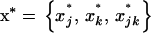. Following Barton and Otto (2005), we focus on the deviations from x*, which occur in the presence of drift. We let 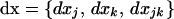describe the vector of these deviations. Thus, at any time t, the vector of allele frequencies and LD can be written as the sum of their deterministic values and the stochastic deviations, x = x* + dx. We begin by deriving a recursion for dx from one generation to the next along a given stochastic trajectory. We then compute the recursions for the expected deviations over all possible trajectories, E[dx]. It is this expected deviation that is of greatest interest to us, as it describes the expected effect, over all possible stochastic outcomes, of drift and selection on allele frequencies and LD during selective sweeps.

Single population:

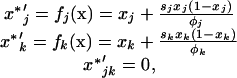
To begin, we describe the case of a single deme (n = 1), where the deterministic trajectory is determined only by recombination and selection. For given values of parameters s_j, s_k, and r_jk, let us write the vector of recursions as , which are three functions that determine the values of the allele frequencies (x_j, x_k) and linkage disequilibrium (x_jk) after selection and recombination (expressions for f_j, f_k, and f_jk are given in Equation A1 in appendix a). After one generation, the deterministic trajectory vector becomes f(x*). In an infinite population with no initial LD and no epistasis (as assumed here), x_jk remains zero, and each locus evolves independently. Consequently, the deterministic trajectory is described by the recursions obtained by setting x_jk to zero in f,

(1)

where 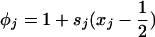and .

For a given trajectory of allele frequency and LD in a finite population, drift creates deviations from the deterministic trajectory that accumulate over time. At a given time t, the finite population is characterized by the vector x = x* + dx, where x* is given by (1). The recursion for the stochastic trajectory x is similar to that for x* except that drift occurs each generation. After selection and recombination, x becomes f(x) = f(x* + dx). Drift then occurs, which corresponds to multinomial sampling from the pool of four haplotypes after selection (this is true even in the diploid case under strict multiplicative selection). Sampling adds a random vector of perturbations to f(x). These perturbations are small as long as the population size is large, and their moments can be found from the multinomial distribution.

After one generation in a finite population (i.e., recombination, selection, and drift), the vector x becomes

(2)

where f(x*) is the value of the deterministic trajectory and is the deviation from the deterministic trajectory in the next generation. From (2), we can write the recursion for deviations from the deterministic trajectory as

(3)

where dx_s = f(x* + dx) − f(x*) represents the value of the vector of deviations after selection and meiosis (before drift).

Approximation in a large population:

Assuming that populations are large enough that all deviations dx remain small (say, of order dx), we can obtain an approximate expression for dx′ by performing a Taylor series expansion of (3) of f(x* + dx) − f(x*) around the deterministic trajectory x* for each of the three recursions f_j, f_k, and f_jk in f. Because the main effect of drift is to introduce variance around the deterministic trajectory, we must keep terms to second order in the deviations in the Taylor Series (see Barton and Otto 2005), yielding

(4)

Because we need a compact notation before analyzing the case of multiple demes, we introduce a vector notation describing each of the deviation terms in (4). We have already described the vector dx, whose terms occur in the first sum of (4). In addition, we require a vector describing the products of deviations, dx_bdx_c, which are O(dx²) terms. Ignoring the order in which the product is taken, there are six elements of this vector, corresponding to the deviations of a pair of variables (x_b, x_c) with b ≤ c ∈ U² (ordering the set U by j < k < jk). For convenience we refer to each of the six pairs of subscripts (b, c) as elements of the set

(5)

The 1 × 6 vector of the products of deviations is thus defined by

(6)

We can then rewrite recursion (4) for the whole system using only matrix notation as

(7)

where D₁ is the 3 × 3 matrix containing the partial derivatives for the first-order terms in the Taylor series (D₁ represents the gradient of f at point x*), and where D₂ is the 3 × 6 matrix containing the different coefficients of the second-order terms in the series. Matrices D₁ and D₂ are given explicitly in appendix a.

Because the recursions for the deviations dx depend on dx², we must also describe recursions for dx². These recursions are obtained by taking the expectation of the products of deviations after one generation, dx_a′dx_b′, (a, b) ∈ V, and approximating the result to second order in the deviations as in (4). The recursion for the expected value of dx² after one generation (recombination, selection, and drift) can then be written as

(8)

where is defined in the same manner as dx² in (6) but with the corresponding stochastic perturbation terms, and where D₃ is the 6 × 6 matrix containing products of first partial derivatives of f at point x* and is obtained by identification in a similar way as D₁ and D₂ (D₃ is also given in appendix a).

Next, we give the distribution of the multinomial perturbation vector ζ under the assumption of a large population size. In the following, we refer to dx and dx² as first- and second-order moments of deviations.

Moments of the multinomial distribution:

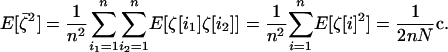
The exact expectations of the perturbations introduced by sampling, E[ζ_a] and E[ζ_aζ_b], are computed from the multinomial distribution and are given in appendix b. To order 1/2N, the effect of sampling on first-order moments simplifies to (one round of drift produces negligible deviation). However, drift does produce variance in the deviations: the effect of sampling on second-order moments is, to order 1/2N,

(9)

where is a 1 × 6 vector with nonzero terms equal to the genetic variances of x_j, x_k, and x_jk, evaluated along the deterministic trajectory. We use the same vector notation as the one defined for dx² in (6).

Because we are interested in evaluating the expected trajectory for the different possible stochastic outcomes, we want to compute the expectations of dx′ and dx²′, which are obtained by taking the expectations of recursions (7) and (8). Note that the elements in the three matrices D₁, D₂, and D₃ are partial derivatives of f evaluated along the deterministic trajectory x*; consequently, they are independent of dx and are not random variables. Thus, the recursion for the expected deviations and product of deviations over one generation is given by

(10a)

(10b)

Recursion (10a) summarizes recursions (4a) and (4b) in Barton and Otto (2005), while recursion (10b) summarizes recursions (5a), (5b), and (5c) in Barton and Otto (2005).

As drift is the initial source of variation and introduces variances of order 1/2N, recursions (10a) and (10b) are of order 1/2N. As long as the stochastic perturbations in dx are small relative to the allele frequencies (i.e., as long as alleles are not close to fixation), they can be approximated by a Gaussian distribution with mean and variance given by recursions (10a) and (10b), respectively (Barton and Otto 2005). These approximate recursions are valid for large populations (i.e., for 1/2N small) and are not valid if the selective sweeps start from a very low allele frequency.

Production of negative linkage disequilibrium:

Here we describe the development of the elements of E[dx], namely the expected deviation from the deterministic trajectory for allele frequencies (E[dx_j] and E[dx_k]) and for the LD (E[dx_jk]). These are the quantities of greatest evolutionary relevance, because they describe the effects of drift on the spread of beneficial alleles and on linkage disequilibria. In particular, E[dx_jk] determines the amount and sign of linkage disequilibrium within the population, because no LD is generated along the deterministic trajectory under multiplicative selection (x_jk* = 0, see Equation 1).

By inspecting Equation 10, note that random genetic drift generates variance around the trajectory [the term c/2N in (10b)], but it does not directly bias the allele frequencies or LD [i.e., drift does not contribute directly to (10a)]. Because D₃ in (10b) contains only zero or positive terms, this variance is converted into positive covariances between deviations in allele frequencies and in LD by the action of selection. Because D₂ in (10a) contains only zero or negative terms, however, this positive covariance between deviations causes, on average, negative deviations in the allele frequency trajectory as well as negative LD. A more detailed interpretation of this process can be found in Barton and Otto (2005).

In short, the interaction of drift and selection generates negative deviations, on average, for both the allele frequencies and LD, relative to their expected values in the absence of drift (deterministic trajectory). In other words, negative genetic associations build up among selected loci (E[dx_jk] < 0) and the selective sweep of beneficial alleles is delayed relative to the time course of selection in an infinite population (E[dx_j] < 0). Because the ultimate source of negative deviations is the variance introduced by drift, the expected deviations are inversely proportional to the population size N and become exceedingly small in very large populations. We now focus on how this process is modified in a subdivided population.

Subdivided population:

Fluctuations within demes around the deterministic trajectory:

We make the key assumption that selection is homogeneous in space so that no linkage disequilibria can be produced deterministically, as would be the case if selection coefficients at the selected loci covaried across demes (Lenormand and Otto 2000). We further assume that all demes start at linkage equilibrium and at the same allele frequencies. Consequently, the initial conditions and deterministic forces are homogeneous, so the deterministic trajectory x* is the same for all demes at any time, and the only difference among demes is due to the stochastic deviations that build up during the selective sweeps occurring in different demes. This homogeneous deterministic trajectory x* equals that of a single population, given by (1). Deviations will differ, however, from one deme to another. We denote as the vector of deviations from x*, along a given stochastic trajectory in deme i. Our aim is to compute the expected value of the vector of average deviations across all demes, which we denote as

(11)

For any variable or vector, we denote the mean taken across all demes with a bar.

As in the single-population model, we also need to compute the recursion for the mean of second-order moments taken across all demes. Using the notation introduced in (5) and (6), we define the vector of the second-order moments, averaged across demes, as

(12)

where, for any couple of variables (x_a, x_b), (a, b) ∈ V, . In our calculations, we also need the product of the average deviations,

(13)

where . For simplicity, we describe the three moments defined in (11), (12), and (13) as the first moment, the within-deme second moment, and the among-deme second moment, respectively.

As in the single-population model, we must compute the recursion over one generation for the expectation of the three moments ( and ) taken across all the possible stochastic trajectories in each deme. To calculate these recursions, we first compute the joint effect of recombination, selection, and drift on the moments, using the results of the single-population model, and then we add the effect of migration. Finally, taking the expectation over all possible trajectories, we derive the recursion for the expected value of the moments over a complete generation in a subdivided population.

Effect of recombination, selection, and drift on the moments in a subdivided population:

Because meiosis, selection, and drift occur independently in each deme, the recursion for the deviation vector dx[i] in any deme i before migration occurs is similar to that given in the single-population model. Consequently, assuming that all demes are large enough, the recursion (7) describes the value of dx[i] along a given stochastic trajectory before migration,

(14)

where dx²[i] is the vector of products of deviations in deme i defined as in (6) and is the perturbation introduced by sampling in deme i on the local vector of allele frequencies and LD. The coefficients in matrices D₁ and D₂ in (14) are evaluated along the deterministic trajectory, common to all demes. As a consequence, the recursion is the same for all demes. Using this fact, it is easy to deduce from (14) the value of the three moments after recombination, selection, and drift, following their definitions given in (11), (12), and (13). Taking the expectation over all possible trajectories, we obtain the expected value of the three moments before migration,

(15)

where is the average across all demes, of the stochastic perturbations that are introduced by drift in each deme i, is the average of the products of these perturbations, and is the product of average perturbations.

Moments of the perturbation vectors:

We now compute the expectations for the effect of n independent multinomial samplings in the n demes on the three moments: , and . The expectations of the sampling vectors in a given deme i are computed from the position along the deterministic trajectory (common to all demes) and from the deme size 2N. Because deme sizes are assumed to be large, we deduce from (9) that, to order 1/2N, , and

(16)

The effect of drift on the within-deme second moment is thus inversely proportional to the local deme size 2N, whether the demes are isolated or connected by migration. This point is important; it ensures that some stochasticity is present even in an infinite population, provided that the population is subdivided into demes of finite size. The among-deme second moments are the products of average deviations by themselves. As drift occurs independently in each deme, each random vector is independent of when i₁ ≠ i₂. Using this independence and the fact that for any i₁, , we obtain, to order 1/2N,

(17)

Sampling has an equivalent effect on the among-deme second moments as it would have on the second moments of a single population of the same total size (i.e., of size 2nN). Consequently, the among-deme second moments will be much smaller than the within-deme second moments in a population composed of a large number of demes (n ≫ 1).

Effect of migration on allele frequencies and linkage disequilibrium in the n-island model:

We next give an exact recursion for the effect of migration on allele frequencies and linkage disequilibrium in an n-island model and the change by migration of the three moments defined in (11), (12), and (13). Details of the derivation are given in appendix b.

We first note that the n-island model can be reduced to a two-island model. Indeed, migration changes haplotype frequencies within a deme, as if this focal deme exchanged migrants with a migrant pool at a rate m_e = mn/(n − 1). Consequently, the effect of migration on allelic frequencies and LD can be derived for any deme, using a two-demes recursion (see, e.g., Barton and Gale 1993) and the values of allele frequencies and LD in the migrant pool (see appendix b). The recursion for the change in allele frequencies and LD averaged across demes (i.e., on 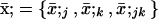) is given by

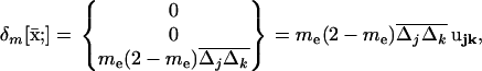(18)

where u_jk = {0, 0, 1} is the unit vector representing the linkage disequilibrium, and where 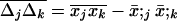is the covariance between allele frequencies at loci j and k, taken across demes, i.e., the spatial covariance between allele frequencies in the whole population. Equation 18 shows that migration (i) does not affect the metapopulation allele frequencies, as expected, and (ii) increases the average linkage disequilibrium per deme by a quantity 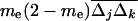each generation. Thus, migration transforms a proportion m_e(2 − m_e) of the spatial covariance between allele frequencies at loci j and k into local linkage disequilibrium between these loci.

We now use recursions for the effect of migration on local (B5) and average (18) allele frequencies and LD to compute the effect of migration on the deviation moments given by (11), (12), and (13). Under homogeneous selection, the effect of selection and recombination on the deterministic trajectory is identical in all demes (differences between demes are only due to stochastic deviations). As a consequence, migration does not affect the deterministic trajectory and changes only the deviations dx[i] in each deme i (δ_m[x_a[i]] = δ_m[dx_a[i]] for any variable a). Using this fact we directly obtain the effect of migration on the first moments ,

(19)

where . The effect of migration on each product of local deviations in deme i is also computed from (B5). We then take the average of these products across demes to obtain the effect of migration on the within-deme second moments, . The resulting expression is simplified by dropping O(dx³) terms (large deme approximation). We then obtain

(20)

where 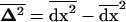can be interpreted as the vector of spatial variances and covariances between all variables. Finally, we similarly compute the effect of migration on the among-deme second moments, using the product of migration effects on average deviations , which is given in (18). Migration has no or negligible effect, o(dx²), on this moment, for allele frequency and LD, respectively: .

Recursions over one generation:

We can now compute the recursion for the expected value of the three moments describing deviations in a population with a life cycle where migration occurs after selection, recombination, and drift. We obtain the overall changes by combining the changes on the three moments due to recombination and selection (15), drift [(16) and (17)], and migration [(19) and (20)]. We obtain a closed recursion system for the expected value of the three moments over one generation [dropping the o(1/2N) for simplicity]:

(21a)

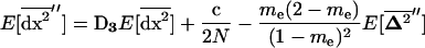(21b)

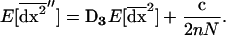(21c)

In (21b), the vector of spatial variances and covariances follows the recursion

(22)

over one generation. in (21a) is the second element in this vector. Because selection occurs independently in each deme, the evolution of recombination depends on local LD between the selected loci. The expectation of this local LD is given by the third element of and its variance across demes is given by the sixth element in . System (21) extends the single-population model (10) to a subdivided population for any migration rate, number of demes, recombination rate, and selection coefficients, provided that the demes remain large and alleles are not close to fixation.

Selection for recombination:

To quantify how recombination evolves in response to the disequilibria generated by the Hill-Robertson effect, we introduce a third locus i modifying r, the recombination rate between the selected loci. As in Barton and Otto (2005), allele 1 at locus i corresponds to a higher recombination rate between loci j and k than allele 0. More precisely, genotypes {0, 0},{1, 0}, and {1, 1} at locus i correspond to recombination rates r − dr, r, and r + dr, respectively. We assume that the three loci are in the order i, j, k and that the recombination rate between i and j is R. We study the change in the frequency x_i at the modifier locus. To include this third locus, we have to keep track of four new variables in our vector recursions: the modifier allele frequency (x_i), the two-locus linkage disequilibria x_ij and x_ik, and the three-locus LD x_ijk. The recursions for the effect of recombination and selection on the seven variables (deterministic function f) are given by Equations A2 in Barton and Otto (2005), for a weak modifier (dr ≪ r).

Extending the method described above for a subdivided population to three loci and computing the effect of migration on the four new variables (see appendix b), we compute a new system of vector recursions that is similar to system (21) but with vectors and matrices of higher dimension (see appendix a), with qualitatively similar effects of migration (described in appendix b).

Comparison with exact simulations:

Simulations were performed to check the analysis and to obtain results for small deme sizes. The simulations followed the same life cycle, using exact recursions for the effects of selection, random mating, meiosis, and migration on haplotype frequencies. Drift was simulated by multinomial sampling within each deme. To study the evolution of recombination, a recombination modifier (third locus) was included with the same effect as described above. We also performed simulations with a sex modifier, in which case individuals {0, 0},{1, 0}, and {1, 1} at locus i were supposed to have sex with probability σ₁, σ₂, and σ₃, respectively. We also introduced the possibility that individuals reproducing sexually produced, e.g., half as many daughters as individuals reproducing asexually (i.e., a twofold cost).

RESULTS

General effect of population subdivision:

We now give a general interpretation of the effect of structure on the system compared to the extreme cases: m_e = 0 (isolated demes) and m_e = 1 (panmictic population). The among-deme second moments [see (21c)] are equivalent to the second moments of deviations in a single population (10b) of size 2nN (the total size of the population); these moments can be interpreted as the variances and covariances of deviations in the migrant pool. The within-deme second moments [see (21b)] are also closely related to the second moments of deviations of a single population. Indeed, using (22), (21b) can be written

(23)

where a_m = 1 − m_e ranges between 0 and 1 as m_e ranges between 0 and 1. Consequently, migration tends to buffer the variances and covariances of deviations produced locally [first term in (23)], bringing them closer to the lower variance produced in a population of total size 2nN [second term in (23)]. Consequently, ranges between the value expected for a single population of size 2N and that for a population of size 2nN. Finally, the first moments (21a) are produced by local variances and covariances, , in the same way as in a single population (see 10a), except that migration also directly favors positive linkage disequilibrium by the admixture of populations with different allele frequencies [contributing the term . Indeed, recursion (22) indicates that any element in (including ) is always positive (all the elements in D₃ are positive). This is true when demes are large (i.e., under our model's assumptions) because the selected alleles spread faster in those demes in which, by chance, positive disequilibrium arises. We see below that this result does not hold for small demes.

As a check, the results for a subdivided population converge upon the results for a single population for extreme values of the migration rate. When m = m_e = 0, recursions (21a) and (21b) reduce to recursions (10a) and (10b) for a single population of size 2N. Conversely, when m = 1 − 1/n (m_e = 1), recursions (21a) and (21b) reduce to recursions (10a) and (10b) for a single population of size 2Nn.

Overall, in a subdivided population of any total size, but with large demes, migration always opposes the creation of negative linkage disequilibrium by drift in the presence of selection. This occurs because (i) the effect of drift is buffered locally by migration and (ii) migration is a direct source of positive LD by admixture. Nevertheless, neither of these effects tends to be large enough to alter the expectation that LD becomes negative.

Infinite subdivided population:

Interestingly, the effects of drift do not disappear even in a population with infinite total size as long as the size of each deme (2N) is finite. Indeed, in the limit as n increases to infinity, the among-deme second moments, scaled to 1/2nN (see 21c), become negligible, so that and recursion (21) simplifies to

(24a)

(24b)

Thus, even in an infinite metapopulation, some variance in deviations is produced by drift within each deme, which causes the expected average disequilibrium across demes to become negative [because of the negative elements of D₂ in (21b)].

We illustrate this result in Figure 1, where we give the maximum absolute value of the average LD per deme in a very large population (2nN ≥ 5 × 10⁶) under weak selection, for various migration and recombination rates. Figure 1 shows that even in a weakly structured population (Nm ≥ 1), a substantial LD can build up in a very large population to a level similar to that expected if the demes were completely isolated as long as gene flow is not too strong (note the steep decrease for large m). Figure 1 also illustrates that, as in a panmictic population, the LD is very low when linkage is loose. Note also that results illustrated in Figure 1 are a lower bound for the LD produced when the number of demes is smaller or when selection is stronger.

Figure 1.

Log-log plot of the maximum absolute value of the average LD between the selected loci, that is reached during the sweeps, for varying migration rate (x-axis) and for three recombination rates (indicated on the graph). The values were obtained from iteration of recursion (21) (lines), from simulations (squares), or from the weak selection approximation (28) (shaded circles). Dashed curves indicate the two limits for the recombination rates r = 0 (top line) and r = (bottom line). For each value of m and r, the number of demes n was chosen large enough (always >500) that further increasing n had very little effect on the result (infinite population limit). Simulation results were averaged over 1800 (m = 0.0002 and 0.002) and 10,000 (m = 0.02) sweeps. Other parameters are s_j = s_k = 0.005, with an initial beneficial allele frequency of 0.1 at both loci and deme size 2N = 10,000.

LD under weak selection:

Loose linkage:

When the processes that reduce linkage disequilibrium are large relative to the processes generating disequilibrium, it is possible to derive an analytical solution for the steady-state level of linkage disequilibrium. This steady-state level depends on the current allele frequencies and is known as a “quasi-linkage equilibrium” (QLE) (Barton and Turelli 1991). When recombination rates are large relative to selection and drift [r ≫ 1/(2N), s_j, s_k], QLE values can be determined, from (21b) and (21c), for the variance in LD within demes, , and among demes, , as well as for the covariances between LD and allele frequencies within demes, , and among demes, (details not shown). For the spatial variances and covariances between allele frequencies, , to reach a steady state, however, it is also required that the migration rate be large relative to selection and drift [m_e ≫ 1/(2N), s_j, s_k], as appears from recursion (22). All spatial covariances in are produced by drift and selection within demes and are reduced by migration. Assuming that the migration rate is large enough, the equilibrium value of these covariances, noted , can be obtained by solving the matrix equation and using recursion (22).

Once the QLE values have been calculated for the second moments, the steady-state level of linkage disequilibrium can be determined from (21a) by setting . To denote this QLE approximation in a population subdivided into n demes of size 2N, we use a hat, . For a single unstructured population of size 2N, Barton and Otto (2005) found that . In a structured population, we find that the linkage disequilibrium falls between the expected LD in a single population of size 2N (the size of the deme) and of size 2nN (the total size of the population) and can be written as

(25)

where

(26)

where a_m = 1 − m_e as in (23) and a_r = 1 − r. As the migration rate increases, α decreases, and the linkage disequilibrium becomes increasingly similar to that expected in a single unstructured population of size 2nN.

Using (26), we can define a QLE population size, N_QLE, according to the population size of an unstructured population that leads to the same expected amount of linkage disequilibrium as that in a structured population. From (25), this equivalent population size is

(27)

Infinite population:

In a population with a very large number of demes, the within-demes and between-demes variances and covariances are equal, [see (24b)]. Assuming that migration is strong enough, these variances and covariances reach an equilibrium . It is then possible, for any recombination rate r, to solve the differential equation for by a continuous time approximation (i.e., under weak selection), using the method presented in Barton and Otto (2005, Equations B4a and B4b). We obtain the average LD per deme after t generations of the selective sweep,

(28)

where α is defined above in (26) and is defined above as the QLE for a panmictic population of the size of the deme (2N). This approximation makes no assumptions on the recombination rate provided that the population has a very large number of demes. As with the QLE approximation in an infinite population (27), this approximation corresponds to the LD produced in a single panmictic population of a finite size 2N /α. The agreement between this approximation and both simulations and recursion (21) is illustrated in Figure 1. The approximation is less accurate with very low migration (m ≤ 0.0001) when the weak structure assumption is no longer met.

QLE for the modifier frequency:

Using the three-locus version of recursion (21), we can compute the expected change in the frequency of a modifier at QLE, assuming that migration and recombination rates are large relative to selection and drift (Figure 2). The result is a complicated function of the parameters describing the population (m, n, 2N) and the genetic map (r and R).

Figure 2.

Value of the average modifier frequency change over time Δx_i, scaled to the modifier effect (dr = 0.03) for three values of the migration rate m indicated on the graph. Lines indicate the values obtained from recursion (21) for three loci and dots indicate the results of simulations with 95% confidence intervals averaged over 10⁷ sweeps. Other parameters are n = 5, 2N = 10,000, r_jk = r_ij = s_j = s_k = 0.1, an initial beneficial allele frequency of 0.01, and an initial modifier frequency x_i = 0.5.

When there is no migration among demes, the predicted change in the modifier collapses down to the results presented in Barton and Otto (2005) for a single unstructured population. With migration, we present results for the special case in which the loci are equidistant (R = r). When migration is weak [but still assuming that m, r ≪ 1, r ≫ 1/(2N), s_j, s_k], the predicted change in the modifier at QLE is to leading order in m and r:

(29)

At the other extreme, in an unstructured population (m_e = 1) with equidistant loci, we retrieve the result presented in Equation 7a of Barton and Otto (2005) for a population of total size 2Nn:

(30)

Integrating the QLE frequency change over the selective sweeps yields the cumulative frequency change and the average per-generation selection coefficient at the modifier locus. Indeed, because the beneficial alleles rise from an initial frequency p₀ to fixation, the cumulative frequency change is obtained by integrating x_j(1 − x_j)x_k(1 − x_k) over time, yielding (1 − p₀)²(1 + 2p₀)/6s.

Figure 3 shows that in a subdivided population with large demes, the frequency change at the modifier locus can be orders of magnitude larger than that in the corresponding panmictic population even for Nm values >1. Figure 3 also illustrates that the QLE approximation captures this behavior under weak selection. As might be expected intuitively, Equation 30 with Nn replaced by N_QLE (27) also provides a reasonable approximation for the frequency change at the modifier locus, although it is less accurate than (29) (see Figure 3). However, these approximations work best in a parameter range where the selection for recombination is weak (for instance, the maximum selection illustrated in Figure 3 is 0.001dr).

Figure 3.

Ratio between the cumulative modifier frequency change, over the selective sweeps, in a structured population, Δx_i(m), and the same frequency change in the absence of structure, Δx_i(m_e = 1), for different values of the migration rate m (x-axis, on log scale). The total population size is kept constant 2nN = 500,000 with either 100 demes of size 2N = 5000 (top curve) or 10 demes of size 2N = 50,000 (bottom curve). The values are obtained with iteration of recursion (21) (solid lines), with the QLE approximation (29) (dashed lines), or with the single-population QLE approximation (29) with a population size 2N_QLE given in (27) (shaded circles). Simulation results averaged over 10,000 sweeps are indicated for the case 2N = 5000 (solid squares). Other parameters are s_j = s_k = r_ij = r_jk = 0.01, with an initial beneficial allele frequency of 0.1, and a modifier effect dr = 0.005 with initial frequency x_i = 0.5.

Overall, we observe similar properties for the rate of change of an allele modifying recombination rates and for the linkage disequilibrium in a subdivided population. In both cases, the predictions fall between those expected in an undivided population whose size is that of the deme (2N) and those in a panmictic population of size 2nN. Furthermore, both the change in the modifier and the linkage disequilibria can be substantial in large, even infinitely large, populations, as long as the population is sufficiently structured.

Smaller deme sizes:

For smaller deme sizes, the deviations from the deterministic trajectory can no longer be assumed small, and our analysis breaks down. We thus turned to simulations to study the development of LD and selection for recombination. We used the same simulations as presented above and each simulation was run until the polymorphism was lost at both selected loci or at the modifier locus (so that no further change in the frequency of the modifier could be expected). For a large population (2nN = 100,000), the effect of deme size on the average per-generation selection coefficient for recombination (scaled to the modifier effect) is illustrated in Figure 4. With realistic values of selection coefficients (s = 0.1) and tight linkage (r = 0.01), the selection coefficient for recombination can be substantial (of the order of 0.1dr). It also shows that our model is a good approximation as long as the deme size 2N is not less than a few thousand. Indeed with smaller demes, the beneficial alleles are often lost temporarily from a deme due to drift, which reduces the amount of local LD. In this context, a small amount of migration favors negative linkage disequilibria directly by admixture (as appeared in simulations, not shown), because it restores polymorphism to individual demes. This can be interpreted more precisely using recursion (18) because this recursion makes no assumption on the deme size so that the average amount of LD per deme produced by admixture is always , even in small demes. When migration is infrequent and demes are small enough that alleles can be locally lost, the Hill-Robertson effect within each deme makes it more likely that the beneficial allele at one locus is lost while the beneficial allele at the other remains, particularly when the selection coefficients at each locus are of the same order. This generates a negative , so that contrary to the large demes case, the effect of admixture, when the population structure is substantial, is to favor negative LD. Overall, the LD produced in a population subdivided into small demes is maximum for an intermediate rate of migration, whereas it is maximum for m = 0 when demes are large. These results are illustrated in Figure 4 (compare deme size above or <1000). When considering small demes, selection for recombination is more efficient in a subdivided population than it would be if demes were either isolated or completely connected.

Figure 4.

Effect of population structure on the per generation selection coefficient on the recombination modifier, s_mod, averaged over the t generations of the selective sweep and scaled by the modifier effect dr. s_mod = Δx_i(t)/(tx_i(1 − x_i)), where Δx_i(t) is the average cumulative modifier frequency change over the selective sweep. The value is given for different deme sizes 2N (x-axis) and migration rates (indicated). Lines show simulation results and dots indicate the prediction from recursion (21) iterated over t = 100 generations (the expected time taken by the selective sweep along the deterministic trajectory). Other parameters are s_j = s_k = 0.1, r_ij = r_jk = 0.01, with an initial beneficial allele frequency of 0.02, and a modifier effect dr = 0.005 with initial frequency x_i = 0.5.

Sex modifiers:

We also performed simulations in which the locus i was a sex modifier. Figure 5 illustrates the effect of population structure as above but with strong selection. Figure 5 also shows that a sex or a recombination modifier has the same behavior. In Figure 6, we also show how the LD generated by the Hill-Robertson effect in a subdivided population selects for increased sex/recombination at a level sufficient to overcome the twofold cost of sex. Note in Figure 6 that increased sex would not be favored in the absence of structure (m_e = 1). These conclusions hold only for a weak modifier effect under very strong selection (s_j = s_k = 1). Indeed, with s_j = s_k = 0.1 and the same parameters as those in Figure 6, a modifier increasing sex does not invade but is less disfavored for intermediate levels of population structure (not shown). However, a weak sex modifier can overcome the twofold cost and invade a structured asexual population of large total size (2nN = 100,000) under weaker selection (for instance, with s = 0.1, see Figure 7) under a wide range of population structures.

Figure 5.

Effect of population structure on modifier final frequency at the end of the sweeps (the initial frequency is 0.5) for different deme sizes 2N (x-axis) and migration rates (indicated) under strong selection (s_j = s_k = 1). The total population size is kept constant, 2nN = 10,000. Lines correspond to a sex modifier with the probability to reproduce sexually (with recombination rate set to ) σ₁ = 0.02, σ₂ = 0.03, and σ₃ = 0.04 for individuals carrying zero, one, or two copies of the modifier, respectively. Dots correspond to a recombination modifier with dr = 0.005 and r_ij = r_jk = 0.015. Initial frequency of selected alleles is 0.01.

Figure 6.

Effect of population structure on a sex modifier final frequency at the end of the sweeps (the initial frequency is 0.5) for different deme sizes 2N (indicated) and migration rates (x-axis, note the log-scale and the value for m = 0) under strong selection (s_j = s_k = 1). The total population size is kept constant, 2nN = 10,000. As in Figure 5, the probability to reproduce sexually (with recombination rate set to ) is σ₁ = 0.02, σ₂ = 0.03, and σ₃ = 0.04 for individuals carrying zero, one, or two copies of the modifier, respectively. In a, there is no cost of sex whereas in b individuals who reproduce sexually produce half as many daughters compared to individuals reproducing asexually (twofold cost). Initial frequency of selected alleles is 0.01.

Figure 7.

Effect of population structure on a sex modifier final frequency at the end of the sweeps. The same as that in Figure 6b is shown (with a twofold cost of sex) but for asexuals vs. weakly sexual organisms (σ₁ = 0, σ₂ = 0.01, and σ₃ = 0.02), weaker selection (s_j = s_k = 0.1), and larger total population size (2nN = 100,000).

DISCUSSION

Drift influences the response to selection of a set of linked loci in a way that is not predicted by the dynamics of each locus considered separately. The interaction of drift and selection tends to build up negative associations between favorable alleles at linked loci (i.e., negative linkage disequilibria), a process known as the HRE. This process generates negative LD in the absence of epistasis, but the latter will also contribute to the development of LD. The negative linkage disequilibrium created by drift in the presence of selection causes beneficial alleles to be associated with deleterious alleles at other loci. Metaphorically, negative LD stores genetic variance in fitness by “hiding” good alleles on bad genetic backgrounds. This variance is restored by the action of recombination. Consequently, modifiers of recombination increase in frequency because they help regenerate good combinations of alleles and rise in frequency along with these combinations.

This stochastic advantage to recombination works in a single population but its magnitude decreases with population size and vanishes when population size tends toward infinity (Barton and Otto 2005). Thus, the stochastic theory for the evolution of sex provides a poor explanation for the maintenance of sex in species with large and unstructured populations. The stochastic theory for sex also fails at the other extreme, in very small populations, because several mutations are unlikely to segregate simultaneously in small populations. Of course, real populations are spatially structured to some extent, and thus we set out to determine the effect of population structure on the stochastic theory for sex. We reached two main conclusions: (i) substantial linkage disequilibrium and selection for recombination can occur in a large—even infinite—population provided that it is subdivided, and (ii) substantial linkage disequilibrium and selection for recombination can also occur in very small demes that are connected by migration, because the polymorphism at the selected loci is maintained at the metapopulation level.

Linkage disequilibria generated by drift with large demes:

When the subpopulations (demes) are large, the LD generated by drift with selection in a subdivided population falls between the LD expected in an isolated deme of size 2N (when m = 0) and that in a single deme of size 2nN (when m = 1). More precisely, when selection is weak relative to migration and recombination, the average LD per deme equals that expected in an unstructured population of size N_QLE, with

where α varies between 0 and 1 [see (26)]. This result holds for any recombination rate in a very large metapopulation [see (28)] and remains accurate for small m-values (see Figure 1).

This apparently simple result summarizes a complex underlying process. In a subdivided population, we can distinguish two sources of LD. The first source of LD is drift with selection, which produces a negative LD on average, as in a single population of size 2N. This process relies upon the creation of variance in LD, which is produced within each deme by drift but is destroyed by migration among demes (see Equation 21b). These antagonistic effects imply that a subdivided population exhibits an intermediate level of variance in LD between a completely structured (m_e = 0) and an unstructured population (m_e = 1). The second source of disequilibrium is migration (admixture), which favors positive LD whenever allele frequencies covary positively across demes (Equation 21a). Indeed, with large demes, we expect this spatial covariance to be positive, because both alleles sweep faster than average in those demes with a positive LD and both alleles sweep slower than average in those demes with a negative LD. Consequently, allele frequencies covary positively across demes, and admixture generates a small amount of positive disequilibrium. However, when selection is homogeneous over space, the effect of admixture is small because it relies on the variance among demes in LD. Indeed, our results indicate that when migration is weak, the variance among demes in LD may be large but a small proportion is converted into positive LD, while when migration is strong, this variance is reduced. Overall, for any level of structure, admixture never overwhelms the Hill-Robertson effect, so that the linkage disequilibrium remains negative, on average.

Overall, the net effect of these two sources of linkage disequilibrium (i.e., drift with selection and admixture) is a negative linkage disequilibrium with a value intermediate between that expected in an unstructured population of size 2N and that of size 2nN. With large demes, gene flow limits the production of negative disequilibrium (i) because the effect of drift is buffered locally by migration and (ii) because migration is a direct source of positive LD through admixture. As in a single population, the resulting LD is larger when selection is strong and equal at both loci and when linkage is tight [in an infinite metapopulation (see 28) or at QLE (see 25) in a finite metapopulation, x_jk is proportional to s_js_k /r³].

Linkage disequilibria generated by drift with small demes:

In a structured population with small demes, the simultaneous fixation of beneficial alleles at both loci is impeded by drift, and one of the beneficial alleles is often lost locally, at least transiently. Therefore, in small isolated populations, there is less scope for the Hill-Robertson effect because of a lack of polymorphism. However, our simulations revealed that a small amount of gene flow among subpopulations is enough to restore the polymorphism at selected loci and allow the Hill-Robertson effect to occur. Indeed, the amount of linkage disequilibrium generated is much higher when small demes are connected by migration than when they are not (see Figure 6, left side). In contrast to the case of large demes, allele frequencies often covary negatively across demes, because the spread of beneficial alleles interferes with the local fixation of other beneficial alleles (Hill and Robertson 1966). Consequently, admixture can itself generate negative disequilibrium, causing the average LD per deme to be larger than that expected either for a set of isolated populations of small size or for a large unstructured population.

Evolution of recombination in a subdivided population:

In the absence of epistasis, increased recombination is favored only if selected loci are negatively associated. Our model shows that, as in a single population, a Hill-Robertson effect occurs in subdivided populations, which generates negative LD and therefore selects for higher rates of recombination. Our results show that population structure has qualitatively similar effects on the frequency of alleles that increase sex or recombination and on the LD between selected loci. When demes are large, the frequency change at the modifier locus is intermediate between the value expected in a single population of size 2N and that in an unstructured population of size 2nN, whereas when demes are small (simulation results), the frequency change at the sex or recombination modifier locus is larger than expected for both migration limits. Unlike a single unstructured population, the genetic associations generated by drift with selection do not vanish when the total population size gets very large or when local deme size gets very small. As a consequence, selection for sex and recombination is effective in a structured population under a broad range of conditions.

Limits of the approach and perspective:

The analytic model developed by Barton and Otto (2005) and extended here to structured populations assumes that within-deme drift is weak enough that beneficial alleles sweep at both loci (i.e., that Ns ≫ 1). Furthermore, both our simulations and analysis assume that initial beneficial allele frequencies are relatively high (p₀ ≥ 1%) and do not vary substantially among demes. These conditions might be met in a weakly structured population undergoing an environmental change with selection on standing variation. In addition, our approximations assume that (i) selection is not too strong relative to migration (and relative to recombination in the case of the QLE approximation) and that (ii) the effect of the modifier on the recombination rate is weak. More theoretical work is needed to relax these assumptions and describe the full spectrum of effects that population structure can have on the development of disequilibria, the spread and fixation of beneficial alleles, and the evolution of recombination. In addition to being often subdivided, natural populations may also experience heterogeneous selection across habitats or epistatic selection across loci. Both factors can generate LD and influence the evolution of recombination (Lenormand and Otto 2000). Including weak epistasis in our model should be possible [by modifying function f in (1)], but modeling heterogeneous selection might be complicated by the fact that we consider constant deterministic trajectories across demes. In any case, the interaction of these factors with population structure remains to be fully explored.

Implications for the theories of the evolution of sex and empirical tests:

Our results suggest that drift could be an important factor favoring sexual reproduction, even in infinite populations, provided that these populations are subdivided into demes of finite size. This could be relatively common in natural populations, which almost always exhibit some level of structure. However, the advantage of sex or recombination due to the HRE can be weak if selection is too weak and the linkage is not tight enough. Consequently, particularly when some cost of sex is included (e.g., increased duration of cell division in isogamous species or twofold cost in anisogamous species), sex/recombination may evolve only in populations of intermediate size and under rapid environmental change with strong selection (Otto and Barton 2001; Otto and Lenormand 2002). We showed that in a metapopulation, a weak sex modifier can overcome the twofold cost over a much broader range of population size and for weaker—but still substantial—selection. Similarly, population structure can increase the advantage of segregation (Agrawal and Chasnov 2001; Otto 2003) and contribute to the maintenance of sexual reproduction. Whether the rate of environmental change and the strength of selection are sufficient in nature for beneficial mutations to drive the evolution of sex remains, however, an open question. Nevertheless, all experimental evidence demonstrating an advantage to recombination relied on either strong artificial selection (see Otto and Lenormand 2002) or abrupt environmental change (Colegrave 2002; Goddard et al. 2005).

Most of the benefit of recombination is gained by a modest amount of sex whereas the twofold cost of sex is proportional to the rate of sex. As a consequence, the evolution of high rates of sex remains difficult to explain. Our results show that given substantial directional multiplicative selection and population structure, a low rate of sex (with the twofold cost) is stable against complete asexuality even in very large populations. The evolution of higher rates of sex seems unlikely in our two-locus study. However, when considering the evolution of sex vs. asex instead of recombination (i.e., when a twofold cost applies), modeling many loci is particularly important as a sex modifier changes recombination rates over the whole genome. As suggested by Barton and Otto (2005), our model could be extended to several loci by summing over pairwise LD. The general matrix recursions [(21) and (24)] that describe the interplay of drift and migration on metapopulation moments should remain unchanged in this context. Although they did not consider a twofold cost, simulations by Iles et al. (2003) showed that adding more loci for a given additive fitness variance resulted in a greater advantage to recombination in a panmictic finite population and in a larger range of population sizes where this advantage is substantial. More work is needed to determine quantitatively the magnitude of the HRE in structured populations with numerous loci and to determine the amount of sex and recombination that is ultimately favored.

An empirical prediction from our analysis is that there should be a positive correlation between levels of population structure and recombination rates. However, using the usual F_st to measure population structure may be misleading. As shown in our model, the effect of structure on linkage disequilibria and on selection for recombination is not simply determined by F_st [see (26), (27), and (29)] but depends in a complicated way on recombination rates, migration rates, and the number and size of demes. Moreover, the power of this approach is weakened by the fact that species will differ in their genomic maps, their history of selection, and their total population size.

Our analysis also predicts how linkage disequilibria should vary across a genome in the presence of selection and drift but in the absence of epistasis. In a weakly structured population, with weak multiplicative selection and loose linkage, using the QLE approximations (26), we can find a simple relationship between F_st, average LD, and the spatial covariance between allele frequencies for any pair of genes separated by r recombination units:

Keeping in mind the various assumptions made in the QLE analysis, there should be a linear relationship between LD and 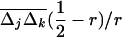measured for different pairs of loci if the Hill-Robertson effect is an important mechanism shaping the disequilibria. This prediction has the nice property that it does not depend on the strength of selection, because is measured, not estimated. However, this spatial covariance might often be too small (≪F_st) to be correctly measured and one needs to know which allele is favored at each locus. This prediction illustrates that the effect of the HRE on LD may be more readily detected in a structured than in a panmictic population.

Summary:

In this article we develop explicit recursions for the effect of drift, selection, and migration in a three-locus system under the island model. These recursions allow us to quantify the effect of structure on the production of linkage disequilibrium between two selected loci by drift in the presence of selection (the Hill-Robertson effect) when deme size is large. We find that, on average, negative disequilibria develop among selected loci. Because of these negative associations among favored alleles, modifier alleles that increase the rate of recombination spread. The rate of this spread is much more substantial in a structured population, contributing to a plausible explanation for why sex and recombination are so ubiquitous.

APPENDIX A: MATRIX NOTATIONS

Explicit expression of the vector function f:

The deterministic changes in allele frequencies and linkage disequilibrium after multiplicative selection and recombination are given by the vector function , from Barton and Otto (2005),

(A1a)

(A1b)

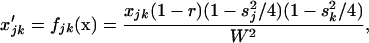(A1c)

where , and 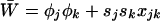are the mean fitnesses of the population, and x = {x_j, x_k, x_jk} is the vector of allele frequencies and LD at the previous generation. (A1c) shows that multiplicative selection alone cannot produce but may change the linkage disequilibrium (x_jk′ is proportional to x_jk).

Exact expressions for the matrices D₁, D₂, and D₃:

The first and second partial derivatives of the vector function f with respect to the three variables x_j, x_k, and x_jk, evaluated along the deterministic trajectory x*, are the elements in matrices D₁, D₂, and D₃. These derivatives can be computed directly from (A1) and are also given in appendix b of Barton and Otto (2005). For each variable in dx (resp. dx²), the corresponding row in matrix D₁ (resp. D₂) is directly computed by identification to the coefficients of the first- (resp. second-) order Taylor series expansion of dx_s = f(x + dx) − f(x), the difference between the stochastic and deterministic trajectories after selection [see (3)]. The 3 × 3 matrix D₁ contains the first partial derivatives of f, which multiply the elements of dx in (4), and equals the gradient of f at point x*,

(A2)

where a_j = 1 − s_j²/4 and a_k = 1 − s_k²/4. Similarly, the 3 × 6 matrix D₂ contains the second partial derivatives of f, which multiply the elements of dx² in (4), as well as the coefficient :

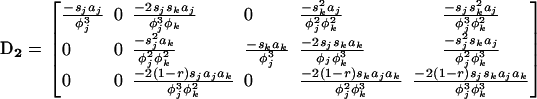(A3)

Note that each term in D₂ is negative, which demonstrates that all variances and covariances of deviations will tend to favor negative deviations with the term D₂dx². Similarly, for each variable in dx², i.e., for each 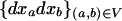, the corresponding row in the 6 × 6 matrix D₃ is obtained by identification to the coefficients of the Taylor series expansion of the products of deviations after selection and recombination (f_a(x + dx) − f_a(x))(f_b(x + dx) − f_b(x)). We then obtain, for the two-locus system:

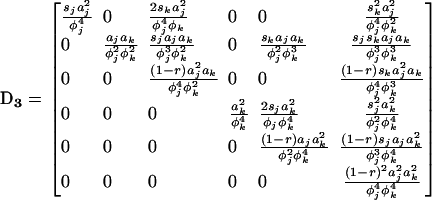(A4)

Matrices D₁, D₂, and D₃ were computed using Mathematica (Wolfram 1991) and are available upon request. The values of x_j and x_k in φ_j and φ_k are evaluated along the deterministic trajectory (x_j = x_j*, x_k = x_k*, and x_jk = x_jk* = 0).

Exact moments introduced by the multinomial sampling:

The adult population is sampled from the surviving juveniles according to a multinomial distribution, as in the standard Wright-Fisher model. Following Barton and Otto (2005), the moments of the multinomial distribution are used to determine the expected values of the perturbations:

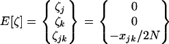(A5)

The variances and covariances of perturbations are given by

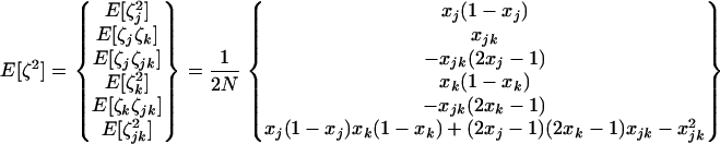(A6)

Large deme size approximation:

The sources of negative deviations E[dx_a] are the variances and covariances of deviations, which are of order O(dx²). Consequently, in our approximation for large population size, terms in dx_a/2N are o(dx²) and are negligible. Therefore, although the actual sampling is made from populations following stochastic trajectories (x_a = x_a* + dx_a), the values of E[ζ_a] and E[ζ_aζ_b] are approximately independent of the actual values of the deviations, dx_a. Thus, the perturbations caused by drift within a generation are determined by the population size and the allele frequencies on the deterministic trajectory. Note that this result explains why terms in E[ζ_adx_b] were dropped from (8). The approximation for large population size of the exact expressions of E[ζ] and E[ζ²] is thus obtained by replacing any x_a by x_a* in (A5) and (A6), so that

(A7)

where is a 1 × 6 vector with the nonzero terms equal to the genetic variances of x_j, x_k, and x_jk, evaluated along the deterministic trajectory.

Three-locus recursions:

When including a modifier locus, i, that modifies the recombination rate between loci j and k, four additional variables are needed to describe the system: the allele frequency at the modifier locus (x_i) and the three additional LD that are defined when including locus i (x_ij, x_ik, and x_ijk). We define new deviation vectors including these variables: the 1 × 7 vector dx of first-order deviations, the 1 × 28 vector of second-order deviations, excluding the repeated products, and the three corresponding metapopulation moments , and . We then follow the same method as that described for the two-locus model. The recursions for the deterministic change, after one round of recombination and selection, for the four additional variables can be found in (A2c)–(A2e) of Barton and Otto (2005). From these recursions, and in the same way as that for the two-locus model, we generate the 7 × 7 matrix D₁, the 7 × 28 matrix D₂, and the 28 × 28 matrix D₃ (available upon request). As in the two-locus model, the multinomial sampling effect is negligible on the vector , while it introduces variance in the vectors and . Finally, the effect of migration on the moments in a subdivided population is exactly the same as that for the two-locus model except for the three-locus linkage disequilibrium dx_ijk (see appendix b).

APPENDIX B: EFFECT OF MIGRATION ON ALLELE FREQUENCIES AND LINKAGE DISEQUILIBRIA IN THE n-ISLAND MODEL

Let us consider a focal deme i, from which a fraction m of individuals emigrate, and into which a comparable number of individuals immigrate from all other demes. Let v[i] be the vector containing the frequencies of multilocus haplotypes in deme i. After migration, the new genotype frequency vector is given by

(B1)

which can also be written

(B2)

where m_e = mn/(n − 1) and is the vector giving the haplotype frequencies in the whole population (or equivalently in the migrant pool). This is exactly the recursion for a two-island system where one deme is the focal deme i and the other is the migrant pool (with haplotype frequency vector ).

This result is valid for any number of loci, but let us first consider the two-locus case. For any variable {x_a}_a∈U at a given time, let us denote the difference between the value of x_a in deme i and the mean of x_a over all demes by . The allele frequencies and linkage disequilibrium in the migrant pool (denoted by the index i = mp) are given by

(B3)

where

(B4)

is the covariance between allele frequencies at loci j and k, taken across demes, i.e., the spatial covariance between allele frequencies in the whole population (cf. also Nei and Li 1973). The recursion for the effect of migration on allele frequencies and LD in the focal deme i is the same as that for the two-island system (given, e.g., in Barton and Gale 1993), where we use the values of x_a[mp] given in (B3) for the other deme (migrant pool). The change due to migration on the vector x[i] of allele frequencies and LD in the focal deme i is thus given by

(B5)

Taking the average across demes of δ_m[x[i]] in (B5), the effect of migration on the average allele frequencies and LD in the whole population (i.e., on ) gives recursion (18). For the three-locus system, recursion (18) has to be changed to include the effect of migration on the other two-locus linkage disequilibria (x_ij and x_ik), which is obtained simply by switching indexes: for example, the change in the linkage disequilibrium dx_ij is . However, the effect of migration on the three-locus linkage disequilibrium x_ijk has to be computed. Following Barton and Turelli (1991) we define the three-locus linkage disequilibrium x_ijk by

(B6)

where, for any diallelic locus l, X_l is a binary variable with value 1 for one of the alleles and 0 for the other, and v_X is the frequency of a given three-locus haplotype {X_i, X_j, X_k} in the population considered (i.e., either the focal deme i or the migrant pool mp). The change in x_ijk for a given deme in the n-island model can be computed as in a two-island system with migration between the deme considered and the migrant pool (deme mp). The value of x_ijk[mp], the three-locus LD in the migrant pool relative to its average across demes , is

(B7)

Then, from (B2), the change in the average x_ijk by migration is

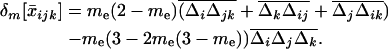(B8)

Taking into account the fact that any Δ_a=dx_a − is of the order of deviations dx_a, and removing O(dx³) terms, we finally obtain the large-deme approximation

(B9)

References

- Agrawal, A. F., and J. R. Chasnov, 2001. Recessive mutations and the maintenance of sex in structured populations. Genetics 158: 913–917. [DOI] [PMC free article] [PubMed] [Google Scholar]
- Barton, N. H., 1995. a A general model for the evolution of recombination. Genet. Res. 65: 123–144. [DOI] [PubMed] [Google Scholar]
- Barton, N. H., 1995. b Linkage and the limits to natural selection. Genetics 140: 821–841. [DOI] [PMC free article] [PubMed] [Google Scholar]
- Barton, N. H., and K. S. Gale, 1993. Genetic analysis of hybrid zones, pp. 13–45 in Hybrid Zones and the Evolutionary Process, edited by R. G. Harrison. Oxford University Press, Oxford.
- Barton, N., and S. P. Otto, 2005. Evolution of recombination due to random drift. Genetics 169: 2353–2370. [DOI] [PMC free article] [PubMed] [Google Scholar]
- Barton, N. H., and L. Partridge, 2000. Limits to natural selection. BioEssays 22: 1075–1084. [DOI] [PubMed] [Google Scholar]
- Barton, N. H., and M. Turelli, 1991. Natural and sexual selection on many loci. Genetics 127: 229–255. [DOI] [PMC free article] [PubMed] [Google Scholar]
- Colegrave, N., 2002. Sex releases the speed limit on evolution. Nature 420: 664–666. [DOI] [PubMed] [Google Scholar]
- Feldman, M. W., F. B. Christiansen and L. D. Brooks, 1980. Evolution of recombination in a constant environment. Proc. Natl. Acad. Sci. USA 77: 4838–4841. [DOI] [PMC free article] [PubMed] [Google Scholar]
- Felsenstein, J., 1974. The evolutionary advantage of recombination. Genetics 78: 737–756. [DOI] [PMC free article] [PubMed] [Google Scholar]
- Felsenstein, J., and S. Yokoyama, 1976. Evolutionary advantage of recombination. 2. Individual selection for recombination. Genetics 83: 845–859. [DOI] [PMC free article] [PubMed] [Google Scholar]
- Fisher, R. A., 1930. The Genetical Theory of Natural Selection. Oxford University Press, Oxford.
- Gerrish, P. J., and R. E. Lenski, 1998. The fate of competing beneficial mutations in an asexual population. Genetica 103: 127–144. [PubMed] [Google Scholar]
- Goddard, M. R., H. Charles, J. Godfray and A. Burt, 2005. Sex increases the efficacy of natural selection in experimental yeast populations. Nature 434: 636–640. [DOI] [PubMed] [Google Scholar]
- Hill, W. G., and A. Robertson, 1966. The effect of linkage on the limits to artificial selection. Genet. Res. 8: 269–294. [PubMed] [Google Scholar]
- Iles, M. M., K. Walters and C. Cannings, 2003. Recombination can evolve in finite populations given selection on sufficient loci. Genetics 165: 2249–2258. [DOI] [PMC free article] [PubMed] [Google Scholar]
- Kondrashov, A. S., 1993. Classification of hypotheses on the advantage of amphimixis. J. Hered. 84: 372–387. [DOI] [PubMed] [Google Scholar]
- Lenormand, T., and S. P. Otto, 2000. The evolution of recombination in a heterogeneous environment. Genetics 156: 423–438. [DOI] [PMC free article] [PubMed] [Google Scholar]
- Maynard Smith, J., 1971. What use is sex? J. Theor. Biol. 30: 319–335. [DOI] [PubMed] [Google Scholar]
- Muller, H. J., 1932. Some genetic aspects of sex. Am. Nat. 66: 118–138. [Google Scholar]
- Nei, M., and W. H. Li, 1973. Linkage disequilibrium in subdivided populations. Genetics 75: 213–219. [DOI] [PMC free article] [PubMed] [Google Scholar]
- Otto, S. P., 2003. The advantages of segregation and the evolution of sex. Genetics 164: 1099–1118. [DOI] [PMC free article] [PubMed] [Google Scholar]
- Otto, S. P., and N. H. Barton, 1997. The evolution of recombination: removing the limits to natural selection. Genetics 147: 879–906. [DOI] [PMC free article] [PubMed] [Google Scholar]
- Otto, S. P., and N. Barton, 2001. Selection for recombination in small populations. Evolution 55: 1921–1931. [DOI] [PubMed] [Google Scholar]
- Otto, S. P., and T. Lenormand, 2002. Resolving the paradox of sex and recombination. Nat. Genet. 3: 252–261. [DOI] [PubMed] [Google Scholar]
- Peck, J. R., 1994. A ruby in the rubbish: beneficial mutations, deleterious mutations and the evolution of sex. Genetics 137: 597–606. [DOI] [PMC free article] [PubMed] [Google Scholar]
- Peck, J. R., J. Yearsley and G. Barreau, 1999. The maintenance of sexual reproduction in a structured population. Proc. R. Soc. Lond. Ser. B Biol. Sci. 266: 1857–1863. [Google Scholar]
- Wolfram, S., 1991. Mathematica. Addison-Wesley, New York.