High-Resolution Association Mapping of Quantitative Trait Loci: A Population-Based Approach

Abstract

In this article, population-based regression models are proposed for high-resolution linkage disequilibrium mapping of quantitative trait loci (QTL). Two regression models, the “genotype effect model” and the “additive effect model,” are proposed to model the association between the markers and the trait locus. The marker can be either diallelic or multiallelic. If only one marker is used, the method is similar to a classical setting by Nielsen and Weir, and the additive effect model is equivalent to the haplotype trend regression (HTR) method by Zaykin et al. If two/multiple marker data with phase ambiguity are used in the analysis, the proposed models can be used to analyze the data directly. By analytical formulas, we show that the genotype effect model can be used to model the additive and dominance effects simultaneously; the additive effect model takes care of the additive effect only. On the basis of the two models, F-test statistics are proposed to test association between the QTL and markers. By a simulation study, we show that the two models have reasonable type I error rates for a data set of moderate sample size. The noncentrality parameter approximations of F-test statistics are derived to make power calculation and comparison. By a simulation study, it is found that the noncentrality parameter approximations of F-test statistics work very well. Using the noncentrality parameter approximations, we compare the power of the two models with that of the HTR. In addition, a simulation study is performed to make a comparison on the basis of the haplotype frequencies of 10 SNPs of angiotensin-1 converting enzyme (ACE) genes.

IN genetics research, one important goal is to locate and identify important genetic variants that are related to complex traits. With the development of dense maps such as single-nucleotide polymorphisms (SNPs) and high-resolution microsatellites in the human genome, enormous amounts of genetic data on human chromosomes are becoming available (International SNP Map Working Group 2001; Kong et al. 2002; International HapMap Consortium 2003; HapMap project, http://www.hapmap.org). The opportunities for a genomewide scan to map complex disease genes are tremendous. It is important to build appropriate models and useful algorithms in association mapping of complex diseases to identify important genetic variants of complex traits, for human, animal, or plant study.

In recent years, there has been great interest in linkage disequilibrium (LD) mapping (or association study) of quantitative traits of complex diseases. One way is to use diallelic markers such as SNPs in analysis. This approach has been receiving much attention and there are quite a lot of references to it in the literature (Fulker et al. 1999; George et al. 1999; Abecasis et al. 2000a,b, 2001; Sham et al. 2000; Fan et al. 2005). Another approach is to use haplotype data that may consist of a set of SNPs (Schaid et al. 2002; Zaykin et al. 2002; Schaid 2004). The haplotype data may provide more information on the relation between DNA variants and complex traits than that of any single SNP. Hence, it is important to investigate models and algorithms that are based on haplotype data. In Schaid et al. (2002) and Zaykin et al. (2002), score tests are proposed for association between complex traits and haplotypes, which can be ambiguous owing to the unknown linkage phase of different haplotypes. In Zaykin et al. (2002), the method is called haplotype trend regression (HTR), which is very close to the method of Schaid et al. (2002) (see Schaid 2004, p. 355, for further explanation). HTR does not assume that haplotype phases are known. Meuwissen and Goddard (2000) introduced a haplotype-based approach, which assumes that haplotype phases are known. In addition, mixed models are used to model the haplotype effect in Meuwissen and Goddard (2000). Morris et al. (2004) used a Markov chain Monte Carlo algorithm based on the shattered coalescent model for fine mapping.

On the other hand, the direct available information is genotypes by current genotyping technology, instead of haplotypes. Hence, it is interesting to build models by directly using genotype information; under these models, the main effects of each marker are modeled, which does not require phase information across the markers. If phase is unknown, presumably the haplotypes would need to be estimated first, using a reconstruction algorithm such as PHASE or EM algorithms (Dempster et al. 1977; M. Stephens et al. 2001; Stephens and Donnelly 2003). This may introduce bias into the subsequent analysis, which would need to be investigated. It is of real interest in making comparison of the genotype-based models and the haplotype-based models. Interestingly, Morris et al. (2004) and Clayton et al. (2004) have observed that the haplotypes at SNPs may be only slightly more advantageous or even less powerful for fine mapping than the corresponding unphased genotypes.

Suppose that a quantitative trait locus (QTL) is located in a chromosome region. In the region, a marker (or two/multiple markers) is (or are) typed. In our previous research, the markers are assumed to be diallelic (Fan and Xiong 2002). In the current article, the markers can be either diallelic or multiallelic. Suppose that a population sample is available. For each individual in the sample, both trait value and genotypes at the markers are observed. We propose two regression models in association mapping of QTL based on population genetic data. One model is the “genotype effect model,” and the other is the “additive effect model.” These two models extend our previous research of high-resolution LD mapping of QTL using diallelic markers (Fan and Xiong 2002). The model can be very easily performed by using any statistical software in data analysis, or it can be easily implemented by widely used language such as C++. By analytical formulas, we show that the genotype effect model can be used to model the additive and dominance effects simultaneously; the additive effect model takes care of additive effect only. On the basis of the two models, F-test statistics are proposed to test association between the QTL and markers. To investigate the robustness of the proposed models and the related F-test statistics, simulation studies are performed to calculate the type I error rates. The noncentrality parameters of F-test statistics are derived to make power calculation and comparison. Moreover, the proposed models are compared with the haplotype trend regression method by simulation study and type I error rate analysis when two diallelic markers are used in the analysis (Zaykin et al. 2002). On the basis of the haplotype frequencies of 10 SNPs of angiotensin-1 converting enzyme (ACE) genes, a simulation study is performed to make power comparison of the proposed models with the haplotype trend regression method (Keavney et al. 1998).

A software, CLAM_QTL, is written in C++ to implement the proposed models and methods, which can be downloaded from http://www.stat.tamu.edu/∼rfan/software.html/.

METHODS

As the first step, we present models and methods by using one marker. Here the marker can be either biallelic or multiallelic. This article extends our previous work (Fan and Xiong 2002). Similar results were worked out independently by colleagues at North Carolina State University, although their language and notations are slightly different (Weir and Cockerham 1977; Nielsen and Weir 1999, 2001). Then, the models and methods are extended to use two/multiple markers in analysis. On the basis of the models, F-test statistics are proposed, and the related noncentrality parameter approximations of the F-tests are derived.

Analysis by one marker:

Population models:

Consider a quantitative trait locus Q, which is located at an autosome. Suppose that there are two alleles Q₁ and Q₂ at the trait locus with frequencies q₁ and q₂, respectively. In a region of the QTL Q, suppose that one marker A is typed, which may be diallelic such as a single-nucleotide polymorphism or may be multiallelic such as a microsatellite marker. Let us denote the alleles of marker A by A₁, …, A_m, where m is the number of alleles. Suppose that the marker A is in Hardy-Weinberg equilibrium (HWE). Let the frequency of A_i be . There are J_A = m(m + 1)/2 possible genotypes, which can be listed as A₁A₁, …, A_mA_m, A₁A₂, …, A₁A_m, …, A_m−1A_m. Accordingly, let β₁₁, …, β_mm, β₁₂, …, β_1m, …, β_m−1,m be the corresponding effects of the listed genotypes on the quantitative trait. Let y be the trait value of an individual with genotype G_A = A_iA_j. Under an assumption of normality, the trait value can be modeled as

(1)

where w is a row vector of covariates such as sex and age, γ is a column vector of regression coefficients of w, and e is the error term. Assume that e is normal N(0, σ_e²). In addition to the covariate effects, there are J_A = m(m + 1)/2 parameters β_ij in model (1), where β_ij = β_ji. Model (1) treats each genotype effect as one parameter. Hence, we call it a genotype effect model. In practice, model (1) may lead to large number of parameters.

Now let us denote the effect of allele A_i as α_i, i = 1, …, m. Suppose the genetic effect is additive in a sense of β_ij = α_i + α_j, i, j = 1, …, m. If an individual has quantitative trait value y and genotype G_A = A_iA_j, model (1) can be modified as

(2)

In addition to the covariate effects, there are m parameters α_i, i = 1, …, m, in model (2). Compared with model (1), model (2) may significantly reduce the number of parameters. Since it models only the additive effect, we call it the additive effect model.

Property of model coefficients and association tests:

As in the traditional quantitative genetics, let a be the effect of genotype Q₁Q₁, d be the effect of genotype Q₁Q₂, and −a be the effect of genotype Q₂Q₂ (Falconer and Mackay 1996). Let α_Q = a + (q₂ − q₁)d be the average effect of gene substitution and δ_Q = 2d be the dominance deviation. In addition, let μ = a(q₁ − q₂) + 2dq₁q₂ be the aggregate effect of the QTL on the trait mean in the population. For i = 1, 2, …, m, let us denote , which are measures of LD between QTL Q and marker A. Here P(Q₁A_i) is the frequency of haplotype Q₁A_i. In appendix a, we show that the regression coefficients of model (1) are given by

(3)

In appendix b, we show that the regression coefficients of model (2) are given by

(4)

From Equations 3 and 4, it is clear that β_ij = α_i + α_j, when δ_Q = 0, i.e., no dominance effect. Suppose that the marker A and the QTL Q are in linkage equilibrium; i.e., . Then Equation 3 implies β_ij = μ; Equation 4 implies that α_i = μ/2. Hence, models (1) and (2) are reduced to

(5)

Assume that the additive genetic effect is significantly present, but the dominance genetic effect is not significantly present; i.e., α_Q ≠ 0 but δ_Q = 0. To test association between the marker A and the QTL Q, one may test hypotheses H_a0: α₁ = ⋯ = α_m vs. H_a1: at least two α_i's are not equal. To see this, note that the hypotheses H_a0: α₁ = ⋯ = α_m is equivalent to , since α_Q is significantly different from 0. Thus, implies and so under H_a0. Hence, the hypotheses H_a0: α₁ = ⋯ = α_m vs. H_a1: at least two α_i's are not equal to each other are equivalent to at least one is not equal to 0. Model (2) can be used to map the QTL by an association analysis.

On the other hand, assume that both additive and dominance genetic effects are significantly present at the putative QTL Q; i.e., α_Q ≠ 0 and δ_Q ≠ 0. To test association between the marker A and the QTL Q, one may test hypotheses H_ad0: β₁₁ = ⋯ = β_mm = β₁₂ = ⋯ = β_1m = ⋯ = β_m−1,m vs. H_ad1: at least two β_ij's are not equal.

Relation to our previous work:

If the marker A has only two alleles A₁ and A₂, Fan and Xiong (2002) proposed the following model in association mapping of the QTL Q,

(6)

where x_A and z_A are dummy random variables defined by

(7)

and α_A and δ_A are regression coefficients of the dummy variables x_A and z_A. The regression coefficients are given by and (Fan and Xiong 2002). It can be shown that model (6) is equivalent to model (1). Actually, the following relations of the regression coefficients of the two models can be shown: , and . Similarly, model (2) is equivalent to y = wγ + μ + x_Hα_A + e, and we have the following relations and . The advantage of model (6) is that the association effect is decomposed into summations of additive and dominance effects if A is diallelic. If A has more than two alleles, model (1) extends model (6), and model (2) extends model y = wγ + μ + x_Hα_A + e.

Regression models:

Assume that N individuals from a population are available for study. Let us list their trait values as y₁, …, y_N and their genotypes as G_A1, …, G_AN. For individual k, let x_ii^(k) be the indicator function of genotype A_iA_i and x_ij^(k) be the indicator function of genotype A_iA_j. That is, they are dummy variables defined by

where i, j = 1, 2, …, m, i ≠ j. Let , k = 1, 2, …, N; i.e., X_k is a column vector of genotype indicator functions of individual k. Here the superscript τ denotes a vector/matrix transpose. Denote . The corresponding regression of model (1) can be written as

(8)

where subscript k indicates the corresponding quantities of individual k.

Similarly, let be the number of alleles A_i of genotype G_Ak, i = 1, 2, …, m, for individual k. That is, is a dummy variable defined by

Denote and . To use model (2) for data analysis, the corresponding regression model is

(9)

F-tests and noncentrality parameter approximations:

It is well known that the additive variance and the dominance variance . Let be the total variance. Assume that there are no covariates. Let us denote , and . Then model (8) can be expressed as y = Xη + e. By standard regression theory, the coefficients can be estimated by . Let H be a (J_A − 1) × J_A matrix defined by

Then, (Hη)^τ = (β₁₁ − β₂₂, …, β₁₁ − β_mm, β₁₁ − β₁₂, …, β₁₁ − β_1m, …, β₁₁ − β_m−1,m). Hence, the hypothesis H_ad0 is equivalent to Hη = (0, …, 0)^τ. From Graybill (1976), Chap. 6, the test statistic of a hypothesis H_ad0 is noncentral F(J_A − 1, N − J_A) defined by

where I_N is the N × N identity matrix. The noncentrality parameter of the above F-statistic is λ_m,ad = (Hη)^τ[H(X^τX)⁻¹H^τ]⁻¹(Hη)/σ². Under the assumption of large sample sizes N, we show in appendix c the approximation

(10)

where R_AQ² is a general measure of the degree of linkage disequilibrium between marker A and the QTL Q defined by (Crow and Kimura 1970; Hedrick 1987; Morton and Wu 1988; Sham et al. 2000). Note that R_AQ² is the χ²-statistic of the m × 2 table of haplotype frequencies of the marker A and trait locus Q. Approximation (10) shows that the noncentrality parameter of test statistics of the null hypothesis of no genetic effects of model (1) is reduced by a factor of for additive variance and by a factor of for dominance variance.

Similarly, let us denote . Then model (9) can be expressed as y = Zψ + e. The coefficients can be estimated by . Let K be a (m − 1) × m matrix defined by

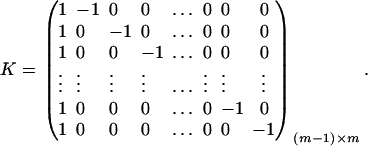Then, (Kψ)^τ = (α₁ − α₂, …, α₁ − α_m). Hence, the hypothesis H_a0 is equivalent to Kψ = (0, …, 0)^τ. From Graybill (1976), Chap. 6, the test statistic of the hypothesis H_a0 is noncentral F(m − 1, N − m) defined by

The noncentrality parameter of the above F-statistic is λ_m,a = (Kψ)^τ[K(Z^τZ)⁻¹K^τ]⁻¹(Kψ)/σ². Under an assumption of large sample sizes N, we show in appendix d the following approximation:

(11)

This approximation (11) shows that the noncentrality parameter λ_m,a is reduced by a factor of for additive variance. The dominance variance is not present in λ_m,a.

Analysis by two/multiple markers:

Population models and association tests:

If genetic data of two/multiple markers are available, models (1) and (2) can be extended for association study of QTL. Most importantly, the data of two/multiple markers may contain phase ambiguity, i.e., phase unknown double heterozygotes. In the following, we generalize models (1) and (2) to directly analyze genetic data of two markers. The principle, actually, can be applied to multiple marker data.

In addition to marker A, assume that a second marker B is typed, which has n alleles denoted by B₁, …, B_n. Suppose that the marker B is also in Hardy-Weinberg equilibrium. Let the frequency of allele B_k be . There are J_B = n(n + 1)/2 possible genotypes, which can be listed as B₁B₁, …, B_nB_n, B₁B₂, …, B₁B_n, …, B_n−1B_n. Let y be the trait value of an individual with genotype G_A at marker A and genotype G_B at marker B. Such as relations (7), define

(12)

If marker A has only two alleles A₁ and A₂, then x_Ai defined above is closely related to x_A, which is defined in (7). Actually, it is easy to see the following relation since .

To extend model (2) by using two markers A and B in the analysis, consider the following model

(13)

In addition to the covariate effects, there are m + n − 1 parameters α, α_Ai, α_Bk, i = 1, …, m − 1, k = 1, …, n − 1 in model (13). To see why model (13) extends model (2), it is worthwhile to note that model (2) is equivalent to . Actually, the quantity implies that if only information of marker A is used in the analysis; thus, α_m = α/2, α_i = α_Ai + α/2, i = 1, …, m − 1. Such as model (2), model (13) takes only the additive effect into account. Hence, we call it an additive effect model. Similarly, model (1) can be extended to

(14)

In addition to the covariate effects, there are J_A + J_B − 1 parameters α, α_Ai, α_Bk, δ_Aij, δ_Bkl in model (14). Model (14) takes both additive and dominance effects into account, and it is called the genotype effect model. Again, model (1) is equivalent to .

Denote X_A = (x_A1, …, x_A(m−1))^τ, X_B = (x_B1, …, x_B(n−1))^τ, and X_A∪B = (X_A^τ, X_B^τ)^τ. Let us denote the additive variance–covariance matrix of the indicator variables x_Ai, x_Bk by . Similarly, let Z_A = (z_A12, …, z_A1m, z_A23, …, z_A2m, …, z_A(m−1)m))^τ, Z_B = (z_B12, …, z_B1n, z_B23, …, z_B2n, …, z_B(n−1)n))^τ, and . Let us denote the dominance variance–covariance matrix of the indicator variables z_Aij, z_Bkl by V_D = Cov(Z_A∪B, Z_A∪B). 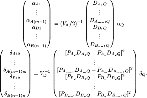For k = 1, 2, …, n, let us denote , which are measures of LD between QTL Q and marker B. In appendix e, we show that the regression coefficients of models (13) and (14) are given by

(15)

The elements of matrices V_A and V_D are provided in appendix e. Equations 15 show that the parameters of LD (i.e., and ) and gene effect (i.e., α_Q and δ_Q) are contained in the regression coefficients. Models (13) and (14) simultaneously take care of the LD and the effects of the putative trait locus Q. The gene substitution effect α_Q is contained only in α_Ai, α_Bk; and the dominance effect δ_Q is contained only in δ_Aij, δ_Bkl. Therefore, V_A is called the additive variance–covariance matrix; and V_D is called the dominance variance–covariance matrix. The model (14) orthogonally decomposes the genetic effect into a summation of additive and dominance effects.

In Fan and Xiong (2002), regression models are proposed for LD mapping of QTL by diallelic markers. Models (13) and (14) extend the models by using multiallelic markers in LD analysis. On the basis of Equations 15, we may use models (13) and (14) to test the association between the trait locus Q and the two markers A and B. Assume that the additive genetic effect is significantly present, but the dominance genetic effect is not significantly present; i.e., α_Q ≠ 0 but δ_Q = 0. To test association between the markers A and B and the QTL Q, one may test hypotheses H_ABa0: α_A1 = ⋯ = α_A(m−1) = α_B1 = ⋯ = α_B(n−1) = 0 vs. H_ABa1: at least one α_Ai, α_Bk is not equal to 0. To see this, note that the hypothesis H_ABa0 is equivalent to , since α_Q is significantly different from 0. On the other hand, assume that both additive and dominance genetic effects are significantly present at the putative QTL Q; i.e., α_Q ≠ 0 and δ_Q ≠ 0. To test association between the markers A and B and the QTL Q, one may test hypothesis H_ABad0: α_A1 = ⋯ = α_A(m−1) = α_B1 = ⋯ = α_B(n−1) = δ_A12 = ⋯ = δ_A1m = ⋯ = δ_A(m−1)m = δ_B12 = ⋯ = δ_B1n = ⋯ = δ_B(n−1)n = 0 vs. H_ABad1: at least one α_Ai, α_Bk, δ_Aij, δ_Bkl is not equal to 0, since both α_Q and δ_Q are significantly different from 0.

Regression models, F-tests, and noncentrality parameter approximations:

Assume that N individuals from a population are available for study, whose trait values are listed as y₁, …, y_N and their genotypes as G_A1, …, G_AN at marker A and G_B1, …, G_BN at marker B. For individual s, let be the corresponding coding functions of genotypes G_As and G_Bs. Let us denote and . Denote α_A∪B = (α, α_A1, …, α_A(m−1), α_B1, …, α_B(n−1))^τ, and δ_A∪B = (δ_A12, …, δ_A(m−1)m, δ_B12, …, δ_B(n−1)n)^τ. The corresponding regression of model (14) can be written as

(16)

Let us denote and and . On the basis of regression (16), one may construct an F-test statistic F_AB,ad to test the null hypothesis H_ABad0 in the same way as constructing F_m,ad or F_m,a (Graybill 1976, Chap. 6). Under the null hypothesis of H_ABad0, F_AB,ad is central to F(J_A + J_B − 2, N − J_A − J_B + 1). Assume the sample size N is large enough that the large sample theory applies. Under the alternative hypothesis of H_ABad1, F_AB,ad is noncentral to F(J_A + J_B − 2, N − J_A − J_B + 1), and it can be shown that the corresponding noncentrality parameter is approximated by

Similarly, an F-test statistic F_AB,a used to test the null hypothesis H_ABa0 can be constructed. Under the null hypothesis of H_ABa0, F_AB,a is central to F(m + n − 2, N − n − m + 1). Under the alternative hypothesis of H_ABa1, F_AB,a is noncentral to F(m + n − 2, N − m − n + 1), and it can be shown that the corresponding noncentrality parameter is approximated by

The haplotype trend regression method:

If only one marker A is used in the analysis, the proposed model (2) is equivalent to the HTR method of Zaykin et al. (2002). However, the proposed models are different from the haplotype trend regression method for two/multiple marker data. Assume that M markers are typed in a region of the trait locus Q. On the basis of the genotypes of the multiple markers, assume that J haplotypes can be determined as h₁, …, h_J with frequencies . For each individual, we may define an expected haplotype score vector as follows (Schaid et al. 2002; Zaykin et al. 2002). The expected haplotype score vector is a column vector of J elements (c₁, …, c_J)^τ based on the genotype combination (G₁, …, G_M) at the markers of an individual. For instance, the score vector is (1, 0, …, 0)^τ if haplotype pair h₁/h₁ is the only possible phase of the genotype combination (G₁, …, G_M). In general, c_j is the conditional probability of a haplotype h_j given genotype combination (G₁, …, G_M) at the markers; i.e.,

In the above equation, the conditional probability P(G₁, …, G_M|h_i, h_k) is 1 if haplotype pair h_i/h_k is a possible phase for the genotype combination (G₁, …, G_M), and P(G₁, …, G_M|h_k, h_j) is 0 otherwise. For each individual, the summation of the expected haplotype scores is equal to 1.

For the purpose of explanation, consider two diallelic markers A and B. Let us denote the two alleles of marker A by A₁, A₂; and denote the two alleles of marker B by B₁, B₂. Table 1 gives the score vector for each genotype combination of markers A and B. To understand the entries of Table 1, it is worthwhile to take genotype combination (G_A = A₁A₁, G_B = B₁B₁) as an example. Two copies of haplotype A₁B₁ can be formed from the genotype combination (G_A = A₁A₁, G_B = B₁B₁). The score for haplotype A₁B₁ is 1 for this genotype combination; and scores for the other three haplotypes are all 0. Denote the genotype of an individual at marker A by G_A and the genotype at marker B by G_B. Let us denote c₁ = P(A₁B₁|G_A = A₁A₂, G_B = B₁B₂) = P(A₁B₁)P(A₂B₂)/[2P(A₁B₁)P(A₂B₂) + 2P(A₁B₂)P(A₂B₁)] = c₄; i.e., c₁ is the conditional probability of a haplotype A₁B₁ given the double heterozygotes (G_A = A₁A₂, G_B = B₁B₂); and . For the double heterozygotes (G_A = A₁A₂, G_B = B₁B₂), the expected scores are c₁, c₂, c₂, c₁ for haplotypes A₁B₁, A₁B₂, A₂B₁, A₂B₂. The scores of the other genotype combinations are provided in Table 1. Then the corresponding model of the haplotype trend regression method can be written as

(17)

where β_i are regression coefficients, and I_i are expected scorings of haplotypes defined in Table 1. It can be seen that model (17) is not equivalent to either proposed model (13) or model (14).

TABLE 1.

Expected scorings I_i, i = 1, 2, 3, 4 of haplotypes of model (17)

	Haplotype and related expected scoring
Genotype (GA, GB)	A1B1, I1	A1B2, I2	A2B1, I3	A2B2, I4
(A1A1, B1B1)	1	0	0	0
(A1A1, B1B2)			0	0
(A1A1, B2B2)	0	1	0	0
(A1A2, B1B1)		0		0
(A1A2, B1B2)	c1	c2	c2	c1
(A1A2, B2B2)	0		0
(A2A2, B1B1)	0	0	1	0
(A2A2, B1B2)	0	0
(A2A2, B2B2)	0	0	0	1

The constants are given by c₁ = P(A₁B₁|G_A = A₁A₂, G_B = B₁B₂) = P(A₁B₁)P(A₂B₂)/[2P(A₁B₁)P(A₂B₂) + 2P(A₁B₂)P(A₂B₁)] and c₂ = – c₁.

In the general case of M markers, let I_j be the expected score of haplotype h_j, j = 1, 2, …, J. In terms of conditional probabilities, I_j can be expressed as

The corresponding model of the haplotype trend regression method can be written as

(18)

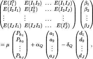
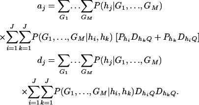
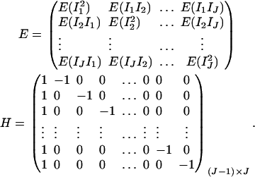
For j = 1, 2, …, J, let us denote , which are measures of LD between QTL Q and the haplotypes. Here P(Q₁h_j) is the frequency of haplotype Q₁h_j. In appendix f, we show that the regression coefficients of model (18) satisfy the matrix equation

(19)

where E(I_iI_k) are given in appendix f, and

From Equations 19, it is clear that model (18) models both the additive and dominance effects. Suppose that the haplotype and the QTL Q are in linkage equilibrium; i.e., . Then Equation 19 implies β₁ = ⋯ = β_J = μ, since and . Hence, model (18) is reduced to (5). To test association between the haplotypes and the trait locus, one may test a null hypothesis β₁ = ⋯ = β_J, and the related F-test statistic can be constructed.

Again, assume that N individuals from a population are available for study with trait values and genotype information. On the basis of regression (18), one may construct an F-test statistic F_HTR to test the null hypothesis β₁ = ⋯ = β_J = μ (Graybill 1976). Under the null hypothesis, F_HTR is central to F(J − 1, N − J). Under the alternative hypothesis that at least two β_j's are not equal to each other, F_HTR is noncentral to F(J − 1, N − J). Assume the sample size N is large enough that the large sample theory applies. Then it can be shown that the corresponding noncentrality parameter is approximated by

where

The advantage of model (17) is that it may model the haplotype effect by parameters β_i. In practice, it is necessary to calculate the expected scorings or haplotype frequencies before building the haplotype trend regression model. Instead, the proposed models (13) and (14) may be used to analyze genetic data directly. Moreover, we have derived analytical formulas to calculate the regression coefficients of the HTR method and the related noncentrality parameter of the test statistic F_HTR. Note that the original article by Zaykin et al. (2002) did not work out this very useful information. Our analytical coefficient equations and related noncentrality parameter approximations can be readily utilized for power evaluation.

RESULTS

Type I error rates:

To evaluate the robustness of the proposed models, we calculate type I error rates of test statistics F_m,ad, F_m,a, F_AB,ad, F_AB,a, and F_HTR at a 0.05 significance level. The results are presented in Tables 2 and 3. Four test cases are considered: null, no major gene effect a = d = 0; additive, additive mode of inheritance a = 1, but no dominant effect d = 0; dominant, dominant mode of inheritance a = d = 1; and recessive, recessive mode of inheritance a = 1 and d = −0.5. The total variance is fixed as σ² = 1.0 and the trait allele frequency is taken as q₁ = q₂ = 0.5 except for that in the null test case. In Table 2, only one marker A is used in analysis; the number m of alleles ranges from 2 to 6. The allele frequencies are given by: when m = 2; when when m = 4; when m = 5; and when m = 6.

TABLE 2.

Type I error rates (percentage) of test statistics F_m,ad and F_m,a at a 0.05 significance level when only one marker A is used in the analysis

			Error rates
No. of alleles	Sample size	Test case	Fm,ad	Fm,a
Diallele, m = 2	N = 200	Null	4.90	4.93
Additive	5.10	4.89
Dominant	4.75	4.98
Recessive	5.03	5.09
Triallele, m = 3	N = 200	Null	4.94	5.18
Additive	5.03	4.92
Dominant	5.07	5.06
Recessive	4.65	4.85
Quadriallele, m = 4	N = 200	Null	4.89	5.29
Additive	4.72	4.69
Dominant	5.03	4.92
Recessive	4.86	4.85
Five alleles, m = 5	N = 200	Null	4.71	5.14
Additive	4.96	4.49
Dominant	5.02	4.94
Recessive	5.04	4.76
Six alleles, m = 6	N = 200	Null	5.02	5.21
Additive	5.23	4.92
Dominant	9.11	5.16
Recessive	7.04	4.97
Six alleles, m = 6	N = 300	Null	4.91	5.36
Additive	5.08	4.98
Dominant	5.39	4.91
		Recessive	5.32	5.11

The total variance is fixed as σ² = 1.0 and the trait allele frequency is taken as q₁ = q₂ = 0.5. The number m of alleles ranges from 2 to 6. The allele frequencies are given by: when m = 2; when m = 3; when m = 4; when m = 5; and when m = 6. Four test cases are considered: null, no major gene effect a = d = 0; additive, additive mode of inheritance a = 1, but no dominant effect d = 0; dominant, dominant mode of inheritance a = d = 1; recessive, recessive mode of inheritance a = 1 and d = –0.5. In each test case, linkage equilibrium is assumed between the QTL Q and the marker A; i.e., .

To calculate the type I error rates, 10,000 data sets are simulated for each test case. Each data set contains either 200 or 300 individuals. In each test case in Table 2, the data sets are generated under an assumption of linkage equilibrium between the QTL Q and the marker A; i.e., . That is, there is no association between the QTL Q and marker A. Utilizing the data sets, we fit either model (8) or model (9), and then calculate the F-test F_m,ad or F_m,a. Because the data sets are generated under the assumption of linkage equilibrium, an empirical test statistic that is larger than the cutting point of the related F-statistic at a 0.05 significance level is treated as a false positive. On the basis of the F-test of either F_m,ad or F_m,a, type I error rates are calculated as the proportions of the 10,000 simulation data sets that give significant results at the 0.05 significance level.

For the test statistic F_m,a, the Table 2 results show that the type I error rates are around the 0.05 nominal significance level in all cases. Hence, the proposed model (9) is robust for data sets of a sample size N = 200. For test statistic F_m,ad, the type I error rates are around the 0.05 nominal significance level when m ≤ 5 for data sets of sample size N = 200. For m = 6 and a sample size N = 200, the type I error rates of test F_m,ad are too big for the dominant and recessive test cases (9.11 and 7.04%, respectively). This is partially due to the large degrees of freedom, J_A − 1 = m(m + 1)/2 − 1 = 20 of test F_m,ad when m = 6; in addition, the high rate of type I error may be also caused by the mode of inheritance, i.e., for the cases of dominant and recessive models. When the sample size increases to N = 300, the type I error rates of test F_m,ad are around the 0.05 nominal significance level for m = 6. Model (8) is less robust than model (9).

In Table 3, two markers A and B are used in the analysis. The numbers m and n of alleles are equal to 2. The allele frequencies are given by and . In each test case, linkage equilibrium is assumed between the QTL Q and the markers A and B; i.e., . Denote , which is the measure of LD between A and B. Here P(A₁B₁) is the frequency of haplotype A₁B₁. Let

(20)

be the measure of the third-order LD (Thomson and Baur 1984). Here P(A₁Q₁B₁) is the frequency of haplotype A₁Q₁B₁. Between marker A and marker B, two situations are considered: (1) linkage equilibrium, i.e., , and (2) linkage disequilibrium, i.e., . No linkage disequilibrium of third order is assumed among markers A and B and the QTL Q; that is, D_AQB = 0. Again, 10,000 data sets are simulated for each test case, and each data set contains 200 individuals. The simulation is done as follows. First, the haplotype frequencies are calculated on the basis of allele frequencies and LD coefficients by relation (20) (Thomson and Baur 1984). Then data sets are simulated using the haplotype frequencies. On the basis of the F-test of either F_AB,ad or F_AB,a or the HTR method, type I error rates are calculated as the proportions of the 10,000 simulation data sets that give significant results at the 0.05 significance level. The Table 3 results show that the type I error rates are around the 0.05 nominal significance level in all cases. Hence, the proposed models (13) and (14) and the HTR method are robust for data sets of a sample size N = 200.

TABLE 3.

Type I error rates (percentage) of test statistics F_AB,ad, F_AB,a, and F_HTR of the haplotype trend regression (HTR) method at a 0.05 significance level when two markers A and B are used in the analysis

LD measure			Error Rates
	Sample size	Test case	FAB,ad	FAB,a	FHTR
0	N = 200	Null	4.90	5.22	5.39
Additive	5.09	4.75	4.77
Dominant	4.62	4.87	4.79
Recessive	5.36	5.12	4.81
0.08	N = 200	Null	5.09	5.23	5.55
Additive	4.92	4.74	4.71
Dominant	4.63	4.84	4.71
		Recessive	5.04	5.02	4.94

The total variance is fixed as σ² = 1.0 and the trait allele frequency is taken as q₁ = q₂ = 0.5. The numbers m and n of alleles = 2. The allele frequencies are given by and . Four test cases are considered: null, no major gene effect a = d = 0; additive, additive mode of inheritance a = 1, but no dominant effect d = 0; dominant, dominant mode of inheritance a = d = 1; recessive, recessive mode of inheritance a = 1 and d = –0.5. In each test case, linkage equilibrium is assumed between the QTL Q and the markers A and B; i.e., . No linkage disequilibrium of third order is assumed among markers A and B and the QTL Q; that is, D_AQB = 0.

Table 4 shows type I error rates (percentages) of test statistics F_ABC,ad, F_ABC,a, and F_HTR at a 0.05 significance level when three diallelic markers A, B, and C are used in the analysis. The measures D_ABC, D_AQC, and D_BQC of the third-order LD are defined as that of D_AQB; the measure of the fourth order is defined accordingly (Bennett 1954). Such as relation (20), the haplotype frequencies at the three markers A, B, and C and at QTL Q are calculated on the basis of allele frequencies and LD coefficients by Weir's (1996, p. 119) relation (3.14). Then data sets are simulated using the haplotype frequencies. Since this article is about population data, one individual may have two copies of haplotypes. Each haplotype is sampled according to the haplotype frequencies. From the Table 4 results, we can see that the proposed models and the HTR method give correct type I errors for data sets of a sample size N = 200.

TABLE 4.

Type I error rates (percentage) of test statistics F_ABC,ad, F_ABC,a, and F_HTR of the haplotype trend regression (HTR) method at a 0.05 significance level when three diallelic markers A, B, and C are used in the analysis

LD measure			Error rates
	Sample size	Test case	FABC,ad	FABC,a	FHTR
0.08	N = 200	Null	5.2	5.35	5.43
Additive	4.98	4.85	4.74
Dominant	4.31	4.68	4.62
Recessive	5.29	5.3	5.27
0.06	N = 200	Null	5.24	5.41	5.39
Additive	5.15	4.89	4.71
Dominant	4.61	5.0	5.03
		Recessive	5.09	4.94	5.08

The total variance is fixed as σ² = 1.0 and the trait allele frequency is taken as q₁ = q₂ = 0.5. The allele frequencies are given by , , and . Four test cases are considered: null, no major gene effect a = d = 0; additive, additive mode of inheritance a = 1, but no dominant effect d = 0; dominant, dominant mode of inheritance a = d = 1; recessive, recessive mode of inheritance a = 1 and d = –0.5. In each test case, linkage equilibrium is assumed between the QTL Q and the markers A, B, and C; i.e., . Moreover, neither third- nor fourth-order linkage disequilibrium is assumed; i.e., D_ABC = D_AQB = D_AQC = D_BQC = D_ABCQ = 0.

Power calculation and comparison:

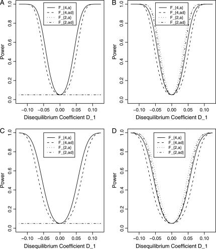
Let h² = σ_ga²/σ² be the heritability. Figure 1 shows power curves of the test statistics F_4,a, F_4,ad, F_2,a, and F_2,ad against the disequilibrium coefficient for a dominant mode of inheritance a = d = 1.0 at a 0.05 significance level based on the approximations of noncentrality parameters λ_m,a and λ_m,ad. F_4,a and F_4,ad are calculated when A has four equal frequency alleles; i.e., . In addition, the measures of LD are given as follows: Figure 1, A and B, , and Figure 1, C and D, . F_2,a and F_2,ad are calculated by collapsing the four alleles to be two alleles: in Figure 1, A and C, alleles A₁ and A₂ are collapsed as one allele, and alleles A₃ and A₄ are collapsed to be the other; in Figure 1, B and D, alleles A₁ and A₃ are collapsed to be one allele, and alleles A₂ and A₄ are collapsed to be the other. For F_2,a and F_2,ad, a simple calculation can show that the measures of LD in Figure 1A are 0, 0; the measures of LD in Figure 1B are ; the measures of LD in Figure 1C are 0, 0; and the measures of LD in Figure 1D are . Hence, the QTL Q is in linkage equilibrium with the marker after collapsing the alleles in Figure 1, A and C. The other parameters are q₁ = 0.50, h² = 0.25, N = 200.

Figure 1.

Power curves of the test statistics F_4,ad, F_4,a, F_2,ad, and F_2,a against the disequilibrium coefficient for a dominant mode of inheritance a = d = 1.0 at a 0.05 significance level. F_4,ad and F_4,a are calculated when marker A has four equal frequency alleles; i.e., . The measures of LD are (A and B) and (C and D) . F_2,ad and F_2,a are calculated by collapsing two of the four alleles: (A and C) alleles A₁ and A₂ are collapsed as one allele, and alleles A₃ and A₄ are collapsed to be the other; (B and D) alleles A₁ and A₃ are collapsed to be one allele, and alleles A₂ and A₄ are collapsed to be the other. The other parameters are q₁ = 0.50, h² = 0.25, N = 200.

From Figure 1, we may see the following:

1. F_4,ad is slightly less powerful than F_4,a, and F_2,ad is slightly less powerful than F_2,a. This is because that test statistic F_m,ad has larger degrees of freedom than those of F_m,a. Note that the noncentrality parameter approximation λ_m,ad of F_m,ad is given by Equation 10. The contribution of the dominance effect is , which depends on both dominance effect d and the magnitude of factor and it can be significant when both of them are large enough. Hence, including a dominance component in the model can improve the power of QTL detection only when the magnitude of is large enough to compensate for the extra degrees of freedom. Note that the quantity is the product of the dominance variance and of the measure R_AQ⁴ of LD. The magnitude of is the result of the dominance variance reduced by a factor . Even when is large, can be small when LD coefficients are not big; i.e., is small.

2. When the measures of LD are high, the power of the test statistics is high. On the other hand, the power is minimal if all measures of LD are close to 0.

3. The dependence of power on measures of LD can also be observed by comparing Figure 1A with Figure 1C, 1B with 1D. The power of F_4,ad and F_4,a in Figure 1A is higher than that of F_4,ad and F_4,a in Figure 1C, respectively; the power of each test statistic in Figure 1B is higher than that of the same test statistic in Figure 1D. This is because the measures of LD in Figure 1A are equal to or higher than those in Figure 1C, and the measures of LD in Figure 1B are equal to or higher than those in Figure 1D.

4. In Figure 1B and Figure 1D, the power of F_4,ad is slightly lower than that of F_2,ad; the power of F_4,a is slightly lower than that of F_2,a.

5. In Figure 1A and Figure 1C, the power of F_2,ad and F_2,a is minimal. This is because measures of LD are 0 after collapsing the alleles in these two graphs.

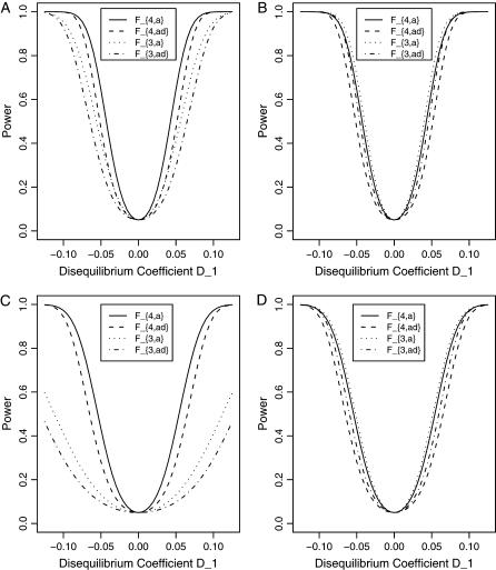
Figure 2 shows power curves of the test statistics F_4,a, F_4,ad, F_3,a, and F_3,ad against the disequilibrium coefficient for a dominant mode of inheritance a = d = 1.0 at a 0.05 significance level. F_4,a and F_4,ad are calculated as those in Figure 1. F_3,a and F_3,ad are calculated by collapsing two of the four alleles to be a new alelle: in Figure 2, A and C, alleles A₁ and A₂ are collapsed as a new one; in Figure 2, B and D, alleles A₁ and A₃ are collapsed to be a new one. For F_3,a and F_3,ad, a simple calculation can show that the measures of LD in Figure 2A are the measures of LD in Figure 2B are the measures of LD in Figure 2C are and the measures of LD in Figure 2D are . Among the features shown in Figure 1, it can be seen that in Figure 2, A and C, the power of F_4,ad is higher than that of F_3,ad, and the power of F_4,a is higher than that of F_3,a. In Figure 2, B and D, the power of F_4,ad is slightly lower than that of F_3,ad, and the power of F_4,a is slightly lower than that of F_3,a. Hence, the way to collapse the alleles has impact on power.

Figure 2.

Power curves of the test statistics F_4,a, F_4,ad, F_3,a, and F_3,ad, against the disequilibrium coefficient for a dominant mode of inheritance a = d = 1.0 at a 0.05 significance level. F_4,ad and F_4,a are calculated when marker A has four equal frequency alleles; i.e., . The measures of LD are the same as those in Figure 1. F_3,ad and F_3,a are calculated by collapsing two of the four alleles: (A and C) alleles A₁ and A₂ are collapsed as a new one; (B and D) alleles A₁ and A₃ are collapsed to be a new one. The other parameters are q₁ = 0.50, h² = 0.25, N = 200.

From Figures 1 and 2, we may see that the power of F_4,a and F_4,ad is relatively stable although it may be slightly lower than that of F_3,a, F_3,ad, F_2,a, and F_2,ad in certain circumstances. However, the power of F_3,a, F_3,ad, F_2,a, and F_2,ad depends heavily on the way to collapse the alleles. This shows the advantage of using multiallelic markers in an association study of QTL detection. For multiallelic marker data, the proposed test statistics F_m,a and F_m,ad can be directly used to test if there is association between the marker and the QTL. As shown in Figures 1 and 2, the test statistic F_m,a is usually more powerful than F_m,ad due to the increase of degrees of freedom of test statistic F_m,ad.

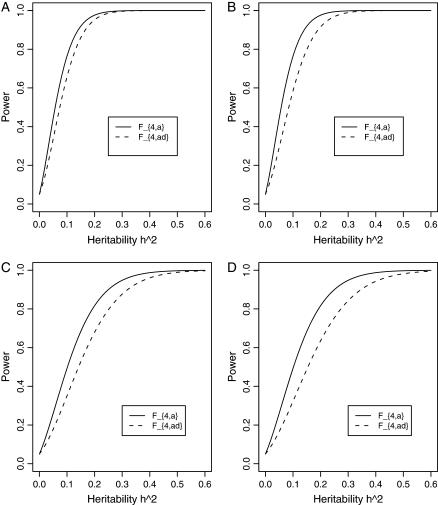
Figure 3 shows power curves of the test statistics F_4,a and F_4,ad against the heritability h² at a 0.05 significance level for a dominant mode of inheritance a = d = 1.0 and for a recessive mode of inheritance a = 1.0, d = −0.5, respectively. As with Figures 1 and 2, Figure 3 is based on noncentrality parameter approximations (10) and (11). In Figure 3, A and B, the power can be high as the heritability h² > 0.1; in these two graphs, the measures of LD are given by . In Figure 3, C and D, the power can be high as the heritability h² > 0.15; in these two graphs, the measures of LD are given by . 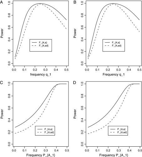Figure 4 shows power curves of the test statistics F_4,a and F_4,ad against the trait allele frequency q₁ or marker allele frequency at a 0.05 significance level. It can be seen that the power depends on both the measures of linkage disequilibrium and the trait allele frequency q₁ or marker allele frequency .

Figure 3.

Power curves of the test statistics F_4,a and F_4,ad against the heritability h² at a 0.05 significance level. (A and C) The curves are plotted for a dominant mode of inheritance a = d = 1.0; (B and D) the curves are plotted for a recessive mode of inheritance a = 1.0, d = −0.5. F_4,a and F_4,ad are calculated when marker A has four equal frequency alleles; i.e., . The measures of LD are given as follows: (A and B) (C and D) . The other parameters are q₁ = 0.50 and N = 250.

Figure 4.

Power curves of the test statistics F_4,a and F_4,ad against the trait allele frequency q₁ or allele frequency at a 0.05 significance level. (A and C) The curves are plotted for a dominant mode of inheritance a = d = 1.0; (B and D) the curves are plotted for a recessive mode of inheritance a = 1.0, d = −0.5. (A and B) The parameters are given by , (C and D) the parameters are given by , . The other parameters are h² = 0.15 and N = 250.

Comparison with the haplotype trend regression method:

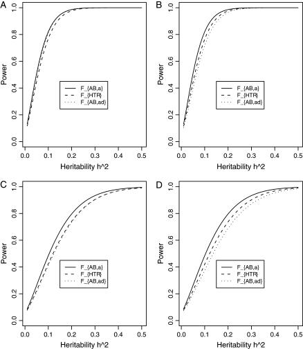
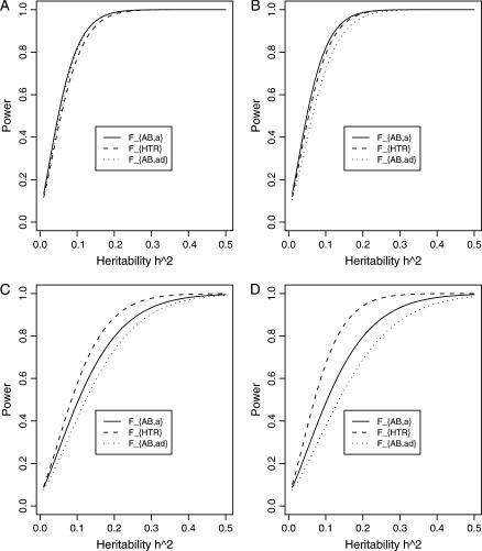
Assume that the two diallelic markers A and B are used in the analysis. Figures 5 and 6 show power curves of the test statistics F_AB,a, F_HTR, and F_AB,ad against the heritability h² at a 0.05 significance level. The related parameters are given in the figure legends. The power curves of the test statistics F_AB,a, F_HTR, and F_AB,ad are calculated on the basis of approximations of noncentrality parameters λ_ABa, λ_HTR, and λ_ABad.

Figure 5.

Power curves of the test statistics F_AB,a and F_AB,ad and F_HTR of the haplotype trend regression method against the heritability h² at a 0.05 significance level, when two diallelic markers A and B are used in the analysis. (A and C) The curves are plotted for a dominant mode of inheritance a = d = 1.0; (B and D) the curves are plotted for an additive mode of inheritance a = 1.0, d = 0. (A and B) The parameters are given by (C and D) the parameters are given by . The other parameters are and N = 200.

Figure 6.

Power curves of the test statistics F_AB,a and F_AB,ad and F_HTR of the haplotype trend regression method against the heritability h² at a 0.05 significance level, when two diallelic markers A and B are used in analysis. All parameters are the same as those in Figure 5 except that (A and B) and (C and D) .

In Figure 5, no third-order linkage disequilibrium is assumed; i.e., D_AQB = 0. In Figure 6, A and B, weak third-order linkage disequilibrium is assumed; i.e., D_AQB = 0.025. It can be seen that the genotype effect model can be less powerful than the HTR method, and the HTR method can be less powerful than the additive effect model in the case of no or weak third-order linkage disequilibrium among the two markers and the QTL (Figure 5 and Figure 6, A and B). In Figure 6, C and D, strong third-order linkage disequilibrium is assumed; i.e., D_AQB = 0.065. In the case that strong third-order linkage disequilibrium exists, the HTR method can be more powerful (Figure 6, C and D).

Note the following fact: in Figure 6, A and B, the maximum of D_AQB is 0.025; in Figure 6, C and D, the maximum of D_AQB is 0.065 (otherwise, some of the haplotype would have negative frequencies). Thus, the simulated power curves of the haplotype trend regression method in Figures 5 and 6 represent the two extreme situations: (1) no third-order linkage disequilibrium (Figure 5) and (2) strongest third-order linkage disequilibrium (Figure 6). In practice, the third-order linkage disequilibrium would exist in a more moderate way that is between the two extremes; and the power of the haplotype trend regression method should be between those of the two extremes. Note that the proposed genotype effect model and additive effect model utilize only the second-order linkage disequilibrium or pairwise linkage disequilibrium. Hence, the powers of F_AB,a and F_AB,ad are the same for Figures 5 and 6.

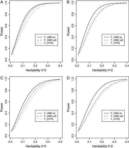
Figure 7 shows power curves of the test statistics F_ABC,a and F_ABC,ad and F_HTR against the heritability h² at a 0.05 significance level, when three diallelic markers A, B, and C are used in the analysis. The related parameters are given in the figure legend. From Figure 7, it can be seen that the power of F_HTR is the lowest. This is due to the large number of degrees of freedom of F_HTR, which is F(7, N − 8), N = 200. In contrast, F_ABC,a is F(3, N − 4), N = 200; and F_ABC,a is F(6, N − 7), N = 200. The low power of F_HTR is most likely due to the biallelic QTL situation that we consider. In the situation of multiple QTL haplotypes and strong LD between QTL and marker haplotypes, the haplotype-based methods are expected to have good power.

Figure 7.

Power curves of the test statistics F_ABC,a and F_ABC,ad and F_HTR of the haplotype trend regression method against the heritability h² at a 0.05 significance level, when three diallelic markers A, B, and C are used in the analysis. (A and C) The curves are plotted for a dominant mode of inheritance a = d = 1.0; (B and D) the curves are plotted for an additive mode of inheritance a = 1.0, d = 0. (A and B) The parameters are given by D_AQ = D_BQ = D_CQ = D_DQ = 0.12, D_AB = D_AC = D_BC = 0.08; (C and D) the parameters are given by D_AQ = D_BQ = D_CQ = D_DQ = 0.10, D_AB = D_AC = D_BC = 0.06. Neither third- nor fourth-order linkage disequilibrium is assumed among markers and the QTL. The other parameters are and N = 200.

Comparison based on ACE haplotype frequencies:

To work on more realistic scenarios, we take the haplotype information of ACE genes as an example. Ten diallelic polymorphisms in the ACE gene spanning 26 kb were genotyped (Keavney et al. 1998). The order of the 10 polymorphisms is T-5991C, A-5466C, T-3892C, A-240T, T-93C, T1237C, G2215A, I/D, G2350A, and 4656(CT)3/2. Table 5 lists 10 haplotypes, where the first 7 are the most frequent haplotypes (http://www.well.ox.ac.uk/∼mfarrall/oxhap_freq.html). For the 10 haplotypes, allele I at marker I/D is always present with allele A at marker G2350A, and allele D at marker I/D is always present with allele G at marker G2350A. Hence, the two markers can be treated as one. Similarly, markers T-5991C and A-5466C can be treated as one; and markers A-240T and T-93C can be treated as one. Therefore, the 10 haplotypes can be considered as containing seven markers.

TABLE 5.

Ranked ACE haplotype frequencies

Haplotype rank	Haplotype identity	Haplotype code	Frequency
1	TATATTGIA3	1111112111	0.352113
2	CCCTCCADG2	2222221222	0.284507
3	TATATCADG2	1111121222	0.087324
4	TACATCADG2	1121121222	0.073239
5	TATATCGIA3	1111122111	0.050704
6	CCCTCCGDG2	2222222222	0.025352
7	TATATTAIA3	1111111111	0.025352
8	CCCTCCGIA3	2222222111	0.008451
9	CCCTCCADG3	2222221221	0.008451
10	TATATCGDG2	1111122222	0.008451

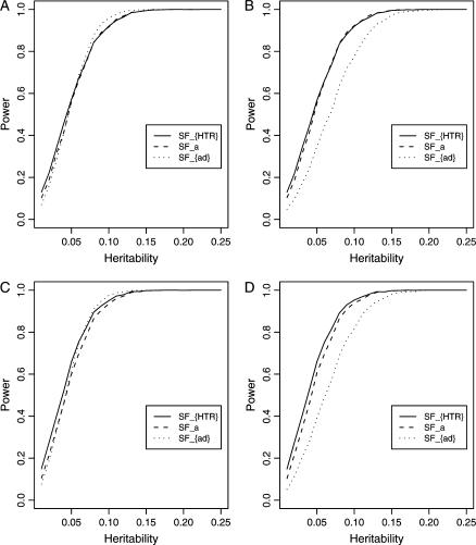
In Abecasis et al. (2000a,b) and Fan et al. (2005), it is found that that markers I/D and G2350A show strongest association with the circulating ACE level. Thus, markers I/D and G2350A are treated as a putative trait locus Q. A quantitative trait of the putative locus Q is simulated for each graph in Figure 8, A–D. The empirical power curves of the test statistics F_HTR, F_a, and F_ad are plotted against the heritability h² at a 0.05 significance level in Figure 8. Here F_a is the test statistic based on the additive effect model, and F_ad is the test statistic based on the genotype effect model. The empirical power curves SF_HTR, SF_a, and SF_ad in Figure 8 are calculated as follows. First, the interval (0.01, 0.25) of the heritability h² is divided into 24 subintervals. Correspondingly, the 24 subintervals lead to 25 end points. For each end point, there is a set of parameters for the power curve. Using the set of parameters, 2500 data sets are simulated for each end point. For each data set, empirical statistics of F_HTR, F_a, and F_ad are calculated. The simulated power is the proportion of the 2500 simulated data sets for which the empirical statistic is larger than the cutting point of the corresponding F-distribution at a 0.05 significance level.

Figure 8.

Empirical power curves of the test statistics F_HTR, F_a, and F_ad against the heritability h² at a 0.05 significance level. The notation SF_a is the empirical power of the F-test statistic based on the additive effect model, SF_ad is the empirical power of the F-test statistic based on the genotype effect model, and SF_HTR is the empirical power of the F-test statistic based on HTR. (A and C) The curves are plotted for a dominant mode of inheritance a = d = 1.0; (B and D) the curves are plotted for an additive mode of inheritance a = 1.0, d = 0. (A and B) Ten haplotypes are used in the simulations; (C and D) 7 haplotypes are used.

In Figure 8, A and C, the curves are plotted for a dominant mode of inheritance a = d = 1.0; in Figure 8, B and D, the curves are plotted for an additive mode of inheritance a = 1.0, d = 0. In Figure 8, A and B, all 10 haplotypes are used in the simulations; in Figure 8, C and D, only the first 7 most frequent haplotypes are used. From Figure 8, A–D, it can be seen that the proposed additive effect model has similar power to that of the HTR method. In Figure 8, A and C, when the dominance effects are present, the genotype effect model has similar power to those of the additive effect model and the HTR method. In Figure 8, B and D, the genotype effect model is less powerful because of the absence of the dominance effect. Hence, the genotype effect model can be useful only if the dominance effect can compensate for the extra degrees of freedom.

Simulation study:

To evaluate the accuracy of the noncentrality parameter approximations, we performed simulations for the power curves in Figures 1, 2, 5, 6, and 7. The results are presented as supplemental information (http://www.genetics.org/supplemental/). It can be seen that the approximations are excellent.

DISCUSSION

In this article, two models, the genotype effect model and the additive effect model, are proposed for high-resolution association mapping of QTL on the basis of population data. The two models extend our previous research, which is based on multiple diallelic markers (Fan and Xiong 2002, 2003; Jung et al. 2005). The genotype effect model is closely linked to the measured genotype approach (Boerwinkle et al. 1986). The very popular genetics software such as Mendel 5.0 is already capable of performing association mapping of QTL by the additive effect model (Cantor et al. 2005; Lange et al. 2005). Surprisingly, there is no research to theoretically show why these two models are valid methods in association mapping of QTL under normal distribution. There are no existing analytical formulas to evaluate the power of the related test statistics. This article shows that the model coefficients are functions of measures of LD; and thus related F-test statistics can be constructed for association study of QTL. In the presence of both additive and dominance effects of the QTL, either the F_m,ad (or F_AB,ad) statistic or the F_m,a (or F_AB,a) statistic can be used. Since the F_m,ad (or F_AB,ad) test statistic has bigger degrees of freedom than those of F_m,a (or F_AB,a), F_m,a (or F_AB,a) can be more powerful. If the extra degrees of freedom of the F_m,ad test can be compensated by magnitude , it can be more powerful than F_m,a.

The formulas of noncentrality parameter approximations (10) and (11) clearly indicate the dependence of the power on the quantity R_AQ² for genetic data. That is, the noncentrality parameter of test statistics of the null hypothesis of no genetic effects is reduced by a factor of for additive variance and by a factor of for dominance variance. If only one diallelic marker A is used in the analysis, both our previous research and the work of colleagues have derived similar formulas to support this argument (Sham et al. 2000; Fan and Xiong 2002, 2003; Fan and Jung 2003; Fan et al. 2005; Jung et al. 2005). This is a good example in the debate on appropriate measures of LD for markers or multiallelic markers (Hedrick 1987; Devlin and Risch 1995; Pritchard and Przeworski 2001; Weiss and Clark 2002). For multiallelic markers or haplotypes, a satisfactory measure of LD has not been derived, as mentioned regarding p306 in Ardlie et al. (2002). For two diallelic loci A and Q, Ardlie et al. (2002) favor using , which is the correlation of alleles at the two loci. For multiallelic marker data, this article extends previous research by providing the definition of R_AQ² and deriving Equations 10 and 11. Hayes et al. (2003) introduced a multilocus approach for estimating LD and past effective size and used chromosome segment homozygosity (CSH), which was introduced in Sved (1971). The dependence of the noncentrality parameter on the quantity has been indicated by our study and also by Sham et al. (2000).

In Fulker et al. (1999), Abecasis et al. (2000a,b, 2001), and Sham et al. (2000), an association between-family and association within-family (“AbAw”) approach is proposed to decompose the genetic association into effects of between pairs and within pairs on the basis of variance component models. The AbAw approach is based on any single diallelic marker. Instead of using a single diallelic marker, we have proposed variance component models using multiple diallelic markers. In our models, the association is decomposed into additive and dominance components (Fan and Xiong 2002, 2003; Fan and Jung 2003; Fan et al. 2005; Jung et al. 2005). In Fan and Jung (2003), Fan et al. (2005), and Jung et al. (2005), we compare our method with the AbAw approach and find that our method is advantageous over the AbAw approach. In model (1) or (2), only one marker is used in model building. If multiple markers or multiallelic markers are available, it is very easy to generalize the models to analyze the data. For instance, model (14) generalizes model (1) if two markers are available in the analysis. Accordingly, model (13) generalizes model (2). If only one marker is used in analysis, the proposed model (2) is equivalent to the haplotype trend regression method by Zaykin et al. (2002), which is very close to the method of Schaid et al. (2002). However, the proposed models are different from the haplotype trend regression method for two/multiple marker data. If both markers are diallelic markers, the genotype effect model can be less powerful than the HTR method, and the HTR method can be less powerful than the additive effect model in the case of no or weak third-order linkage disequilibrium among the two markers and the QTL. If strong third-order linkage disequilibrium exists, the HTR method can be more powerful.

Basically, the proposed models are genotype based. The models can be used to analyze directly any number of markers, and the markers can be either diallelic or multiallelic. By a simulation study based on ACE haplotype frequencies, we show that the proposed additive effect models have similar power to that of the haplotype-based HTR method. In the meantime, the proposed models enjoy the simplicity of not needing to estimate the expected haplotype scorings; in contrast, the HTR method needs to calculate the expected haplotype scorings before building the models. The proposed models decompose the main marker effects into a summation of additive and dominance effects. In the presence of haplotype effects, it is important to estimate the haplotype effects and haplotype-based methods are more relevant (Stram et al. 2003; Tregouet et al. 2004).

One potential problem of this generalization is that the number of parameters can be very big. Then, one needs to select important alleles in the analysis and search for important genetic variants that are truly associated with the genetic traits. At first glance, model (1), (2), (13), or (14) seems too complicated and contains too many terms. However, the models are not intimidating at all if one takes into account the recent discovery of haplotype structure in the human genome. Although a haplotype block may contain many SNPs, it takes only a few SNPs to uniquely identify each of the haplotypes in the block. Within a block, there are only two to four common haplotypes (Arnheim et al. 2003; Daly et al. 2001; Goldstein 2001; Patil et al. 2001; Reich et al. 2001; Rioux et al. 2001; J. C. Stephens et al. 2001; Gabriel et al. 2002; Nordborg and Tavaré 2002; Phillips et al. 2003). This implies that model (1), (2), (13), or (14) contains a few terms and hence is manageable. Moreover, model (1) or (2) already takes the haplotype structure into account and is potentially more powerful. In practice, one may want to collapse some alleles to reduce the number of parameters. However, the collapsing process may decrease linkage disequilibrium and therefore result in loss of power. The proposed regression models can be fitted to alleviate the problem.

In the mathematical derivations, we make the assumption of HWE. It is unclear how to construct tests reflecting deviations from HWE and this requires further research. In addition, we illustrate that the false-positive rate of the genotype effect test is too high for more than five alleles in a sample of 200 individuals. This is obviously due to the large numbers of possible genotypes and hence to sparseness in the contingency table. This problem could be overcome by using exact tests or permutation procedures.

The models of this article are based on population data. Suppose that both population and pedigree data including sibships are available. Then, model (1) or (2) can be generalized to perform high-resolution combined LD mapping and a linkage study of QTL by variance component models in the spirit of our previous work. In fact, we may generalize regression (1) or (2) by adding the polygenic effect to fit the data. Moreover, log-likelihoods can be constructed on the basis of variance component models. This will generalize our research by using either diallelic/multiallelic markers or haplotypes in a combined analysis of population and pedigree data. It is well known that association study-based population data are prone to false positives, due to the population stratification and population history. A valid approach would be to find linkage information by using pedigree data to locate the QTL on a broad chromosome region. Then, a combined linkage and association mapping can be performed for fine mapping of the genetic traits on the basis of both population and pedigree data (Fan and Xiong 2003). This would be more likely to overcome the drawbacks of separate analysis of either a linkage study or association mapping: low resolution of linkage analysis and high false-positive rates in the association study. In the meantime, it is more likely to take advantage of the two methods: the low false-positive rates of linkage analysis and the high resolution of the association-mapping method.

APPENDIX A

For an individual of a population with trait values y and genotype G_A at marker A, let x_ii be an indicator function of genotype A_iA_i and x_ij be an indicator function of genotype A_iA_j. That is, they are dummy variables defined by

where i, j = 1, 2, …, m, i ≠ j. Then model (1) can be rewritten as

(A1)

Note that . Given Equation A1, taking expectation of yx_ii leads to . On the other hand, a true random-effect model describing the trait value is y = wγ + g + e, where

Utilizing and gives

(A2)

Equating the above quantity to shows Equation 3 when i = j.

If i ≠ j, . Multiplying at both sides of Equation A1 by x_ij and taking the expectation lead to E(yx_ij) = E(x_ij)[wγ + β_ij]. Again, utilizing , , , and gives

(A3)

Equating the above quantity to shows Equation 3 when i ≠ j.

APPENDIX B

For an individual with trait values y and genotypes G_A at marker A, let z_i be the number of alleles A_i of genotype G_A, i = 1, 2, …, m. That is, z_i is a dummy variable defined by

Then model (2) can be rewritten as

(B1)

Multiplying both sides of expression (B1) by z_i and taking the expectation lead to

(B2)

The elements of the matrix on the left-hand side of the above equation can be calculated as follows: . For i ≠ j, the expectation . For the elements on the right-hand side, Equations A2 and A3 lead to , since . Plugging the above quantities into matrix Equation B2 gives Equation 4 as

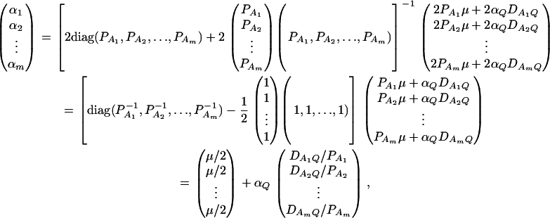where diag(…) denotes a diagonal matrix; e.g., is

In the above calculation, we use a fact of the inverse matrix (M + ab^τ)⁻¹ = M⁻¹ − (M⁻¹a)(b^τM⁻¹)/(1 + b^τM⁻¹a).

APPENDIX C

Denote a vector . If the sample size N is large enough, the large number law implies the approximation

(C1)

where is a diagonal matrix, whose elements on the diagonal are given by the elements of . That is, if , then . Let H be a (J_A − 1) × J_A matrix defined by

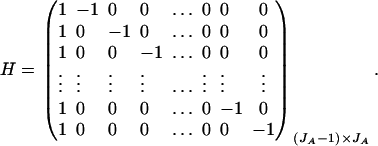Then, (Hη)^τ = (β₁₁ − β₂₂, …, β₁₁ − β_mm, β₁₁ − β₁₂, …, β₁₁ − β_1m, …, β₁₁ − β_m−1,m). From approximation (C1), we have the approximation

where . Applying a fact of inverse matrix (M + ab^τ)⁻¹ = M⁻¹ − (M⁻¹a)(b^τM⁻¹)/(1 + b^τM⁻¹a) again, we have

The noncentrality parameter is given by

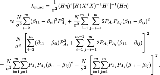(C2)

From Equation 3, we have

Utilizing relation , we have

Plugging the above equation into (C2), we have

Note that , and so . Hence, the noncentrality parameter approximation (10) is valid.

APPENDIX D

The large number law implies the following approximation:

In the above approximation, the quantities E(z_iz_j) in appendix b are used. Applying a fact of inverse matrix (M + ab^τ)⁻¹ = M⁻¹ − (M⁻¹a)(b^τM⁻¹)/(1 + b^τM⁻¹a), the inverse is

Let K be a (m − 1) × m matrix defined by

Then, (Kψ)^τ = (α₁ − α₂, …, α₁ − α_m). On the other hand, we have the approximation

whose inverse is given by

Therefore, an approximation of the noncentrality parameter is given by

Equation 4 implies that . Thus, the noncentrality parameter

APPENDIX E

For i = 1, 2, …, m, k = 1, …, n, let us denote , which are measures of LD between markers A and B. Here P(A_iB_k) is frequency of haplotype A_iB_k. It can be shown that for i ≠ j, k ≠ l, j ≠ j′, l ≠ l′, (i, j) ≠ (i′, j′), (k, l) ≠ (k′, l′),

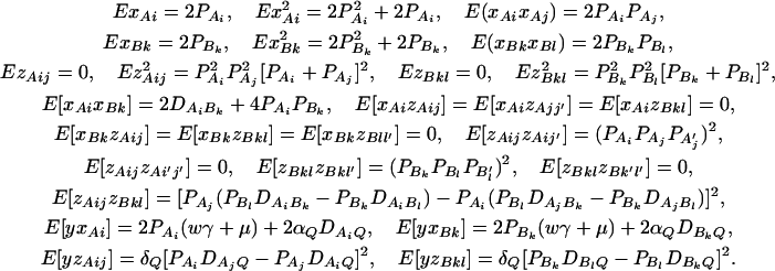(E1)

The quantities in (E1) imply that

Since EZ_A∪B is a vector of 0's by the quantities in (E1), it can be shown that V_D = Cov(Z_A∪B, Z_A∪B) = E(Z_A∪BZ_A∪B^τ). Moreover, the quantities in (E1) imply that the covariance matrix Cov(X_A∪B, Z_A∪B) is a 0 matrix.

Taking variance–covariance between y and x_Ai, x_Bk, z_Aij, z_Bkl on the basis of relation (14), we may get the regression coefficients (15) of models (13) and (14).

APPENDIX F

Multiplying both sides of expression (18) by I_j and taking the expectation lead to

(F1)

The elements of the matrix on the left-hand side of the above equation can be calculated as follows:

The elements on the right-hand side are given by

where

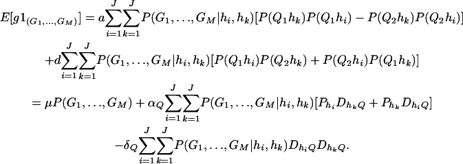Plugging the above quantities into matrix Equation F1 gives Equation 19.

References

- Abecasis, G. R., L. R. Cardon and W. O. C. Cookson, 2000. a A general test of association for quantitative traits in nuclear families. Am. J. Hum. Genet. 66: 279–292. [DOI] [PMC free article] [PubMed] [Google Scholar]
- Abecasis, G. R., W. O. C. Cookson and L. R. Cardon, 2000. b Pedigree tests of linkage disequilibrium. Eur. J. Hum. Genet. 8: 545–551. [DOI] [PubMed] [Google Scholar]
- Abecasis, G. R., W. O. C. Cookson and L. R. Cardon, 2001. The power to detect linkage disequilibrium with quantitative traits in selected samples. Am. J. Hum. Genet. 68: 1463–1474. [DOI] [PMC free article] [PubMed] [Google Scholar]
- Ardlie, K. G., L. Kruglyak and M. Seielsstad, 2002. Patterns of linkage disequilibrium in the human genome. Nat. Rev. Genet. 3: 299–309. [DOI] [PubMed] [Google Scholar]
- Arnheim, N., P. Calabrese and M. Nordborg, 2003. Review article: hot and cold spots of recombination in the human genome: the reason we should find them and how this can be achieved. Am. J. Hum. Genet. 73: 5–16. [DOI] [PMC free article] [PubMed] [Google Scholar]
- Bennett, J. H., 1954. On the theory of random mating. Ann. Eugen. 18: 311–317. [DOI] [PubMed] [Google Scholar]
- Boerwinkle, E., E. Chakraborty and C. F. Sing, 1986. The use of measured genotype information in the analysis of quantitative phenotype in man. I. Models and analytical methods. Ann. Hum. Genet. 50: 181–194. [DOI] [PubMed] [Google Scholar]
- Cantor, R. M., G. K. Chen, P. Pajukanta and K. Lange, 2005. Association testing in a linked region using large pedigrees. Am. J. Hum. Genet. 76: 538–542. [DOI] [PMC free article] [PubMed] [Google Scholar]
- Clayton, D., J. Chapman and J. Cooper, 2004. The use of unphased multilocus genotype data in indirect association studies. Genet. Epidemiol. 27: 415–428. [DOI] [PubMed] [Google Scholar]
- Crow, J. F., and M. Kimura, 1970. An Introduction to Population Genetics Theory. Harper & Row, New York.
- Daly, M. J., J. D. Rioux, S. F. Schaffner, T. J. Hudson and E. S. Lander, 2001. High-resolution haplotype structure in the human genome. Nat. Genet. 29: 229–232. [DOI] [PubMed] [Google Scholar]
- Dempster, A. P., N. M. Laird and D. B. Rubin, 1977. Maximum likelihood from incomplete data via the EM algorithm. J. R. Stat. Soc. Ser. B 39: 1–38. [Google Scholar]
- Devlin, B., and N. Risch, 1995. A comparison of linkage disequilibrium measures for fine-scale mapping. Genomics 29: 311–322. [DOI] [PubMed] [Google Scholar]
- Falconer, D. S., and T. F. C. Mackay, 1996. Introduction to Quantitative Genetics, Ed. 4. Longman, London. [DOI] [PMC free article] [PubMed]
- Fan, R. Z., and J. S. Jung, 2003. High resolution joint linkage disequilibrium and linkage mapping of quantitative trait loci based on sibship data. Hum. Hered. 56: 166–187. [DOI] [PubMed] [Google Scholar]
- Fan, R. Z., and M. M. Xiong, 2002. High resolution mapping of quantitative trait loci by linkage disequilibrium analysis. Eur. J. Hum. Genet. 10: 607–615. [DOI] [PubMed] [Google Scholar]
- Fan, R. Z., and M. M. Xiong, 2003. Combined high resolution linkage and association mapping of quantitative trait loci. Eur. J. Hum. Genet. 11: 125–137. [DOI] [PubMed] [Google Scholar]
- Fan, R. Z., C. Spinka, L. Jin and J. S. Jung, 2005. Pedigree linkage disequilibrium mapping of quantitative trait loci. Eur. J. Hum. Genet. 13: 216–231. [DOI] [PubMed] [Google Scholar]
- Fulker, D. W., S. S. Cherny, P. C. Sham and J. K. Hewitt, 1999. Combined linkage and association sib-pair analysis for quantitative traits. Am. J. Hum. Genet. 64: 259–267. [DOI] [PMC free article] [PubMed] [Google Scholar]
- Gabriel, S. B., S. F. Schaffner, H. Nguyen, J. M. Moore, J. Roy et al., 2002. The structure of markers in the human genome. Science 296: 2225–2229. [DOI] [PubMed] [Google Scholar]
- George, V., H. K. Tiwari, X. F. Zhu and R. C. Elston, 1999. A test of transmission/disequilibrium for quantitative traits in pedigree data, by multiple regression. Am. J. Hum. Genet. 65: 236–245. [DOI] [PMC free article] [PubMed] [Google Scholar]
- Goldstein, G. B., 2001. Islands of linkage disequilibrium. Nat. Genet. 29: 109–111. [DOI] [PubMed] [Google Scholar]
- Graybill, F. A., 1976. Theory and Application of the Linear Model. Wadsworth & Brooks/Cole Advanced Books & Software, Pacific Grove, CA.
- Hayes, B. J., P. M. Visscher, H. C. McPartlan and M. E. Goddard, 2003. Novel multilocus measure of linkage disequilibrium to estimate past effective population size. Genome Res. 13: 635–643. [DOI] [PMC free article] [PubMed] [Google Scholar]
- Hedrick, P. W., 1987. Gametic disequilibrium measures: proceed with caution. Genetics 117: 331–341. [DOI] [PMC free article] [PubMed] [Google Scholar]
- International HapMap Consortium, 2003. The International HapMap Project. Nature 426: 789–796. [DOI] [PubMed] [Google Scholar]
- International SNP Map Working Group, 2001. A map of human genome sequence variation containing 1.42 million single nucleotide polymorphisms. Nature 409: 928–933. [DOI] [PubMed] [Google Scholar]
- Jung, J. S., R. Z. Fan and L. Jin, 2005. Combined linkage and association mapping of quantitative trait loci by multiple markers. Genetics 170: 881–898. [DOI] [PMC free article] [PubMed] [Google Scholar]
- Keavney, B., C. A. McKenzie, J. M. Connell, C. Julier, P. J. Ratcliffe et al., 1998. Measured haplotype analysis of the angiotension-1 converting enzyme gene. Hum. Mol. Genet. 7: 1745–1751. [DOI] [PubMed] [Google Scholar]
- Kong, A., D. F. Gudbjartsson, J. Sainz, G. M. Jonsdottir, S. A. Gudjonsson et al., 2002. A high resolution recombination map of the human genome. Nat. Genet. 31: 241–247. [DOI] [PubMed] [Google Scholar]
- Lange, K., J. S. Sinsheimer and E. Sobel, 2005. Association testing with Mendel. Genet. Epidemiol. 29: 36–50. [DOI] [PubMed] [Google Scholar]
- Meuwissen, T. H. E., and M. E. Goddard, 2000. Fine mapping of quantitative trait loci using linkage disequilibria with closely linked marker loci. Genetics 155: 421–430. [DOI] [PMC free article] [PubMed] [Google Scholar]
- Morris, A. P., J. C. Whittaker and D. J. Balding, 2004. Little loss of information due to unknown phase for fine-scale linkage-disequilibrium mapping with single-nucleotide-polymorphism genotype data. Am. J. Hum. Genet. 74: 945–953. [DOI] [PMC free article] [PubMed] [Google Scholar]
- Morton, N. E., and D. Wu, 1988. Alternative bioassays of kinship between loci. Am. J. Hum. Genet. 42: 173–177. [PMC free article] [PubMed] [Google Scholar]
- Nielsen, D. M., and B. S. Weir, 1999. A classical setting for associations between markers and loci affecting quantitative traits. Genet. Res. 74: 271–277. [DOI] [PubMed] [Google Scholar]
- Nielsen, D. M., and B. S. Weir, 2001. Association studies under general disease models. Theor. Popul. Biol. 60: 253–263. [DOI] [PubMed] [Google Scholar]
- Nordborg, M., and S. Tavaré, 2002. Linkage disequilibrium: what history has to tell us. Trends Genet. 18: 83–90. [DOI] [PubMed] [Google Scholar]
- Patil, N. P., A. J. Berno, D. A. Hinds, W. A. Barrett, J. M. Doshi et al., 2001. Blocks of limited haplotype diversity revealed by high-resolution scanning of human chromosome 21. Science 294: 1719–1723. [DOI] [PubMed] [Google Scholar]
- Phillips, M. S., R. Lawrence, R. Sachidanandam, A. P. Morris, D. J. Balding et al., 2003. Chromosome-wide distribution of markers and the role of recombination hot spots. Nat. Genet. 33: 382–387. [DOI] [PubMed] [Google Scholar]
- Pritchard, J. K., and M. Przeworski, 2001. Linkage disequilibrium in humans: model and data. Am. J. Hum. Genet. 69: 1–14. [DOI] [PMC free article] [PubMed] [Google Scholar]
- Reich, D. E., M. Cargill, S. Bolk, J. Ireland, R. C. Sabett et al., 2001. Linkage disequilibrium in the human genome. Nature 411: 199–204. [DOI] [PubMed] [Google Scholar]
- Rioux, J. D., M. J. Daly, M. S. Silverberg, K. Lindblad, H. Steinhart et al., 2001. Genetic variation in the 5q31 cytokine gene cluster confers susceptibility to Crohn disease. Nat. Genet. 29: 223–228. [DOI] [PubMed] [Google Scholar]
- Schaid, D. J., 2004. Evaluating associations of haplotypes with traits. Genet. Epidemiol. 27: 348–364. [DOI] [PubMed] [Google Scholar]
- Schaid, D. J., C. M. Rowland, D. E. Tines, R. M. Jacobson and G. A. Poland, 2002. Score tests for association between traits and haplotypes when linkage phase is ambiguous. Am. J. Hum. Genet. 70: 425–434. [DOI] [PMC free article] [PubMed] [Google Scholar]
- Sham, P. C., S. S. Cherny, S. Purcell and J. K. Hewitt, 2000. Power of linkage versus association analysis of quantitative traits, by use of variance-components models, for sibship data. Am. J. Hum. Genet. 66: 1616–1630. [DOI] [PMC free article] [PubMed] [Google Scholar]
- Stephens, J. C., J. A. Schneider, D. A. Tanguay, J. Choi, T. Acharya et al., 2001. Haplotype variation and linkage disequilibrium in 313 human genes. Science 293: 489–493. [DOI] [PubMed] [Google Scholar]
- Stephens, M., and P. Donnelly, 2003. A comparison of Bayesian methods for haplotype reconstruction from population genotype data. Am. J. Hum. Genet. 73: 1162–1169. [DOI] [PMC free article] [PubMed] [Google Scholar]
- Stephens, M., N. Smith and P. Donnelly, 2001. A new statistical method for haplotype reconstruction from population data. Am. J. Hum. Genet. 68: 978–989. [DOI] [PMC free article] [PubMed] [Google Scholar]
- Stram, D. O., C. A. Haiman, J. N. Hirschhorn, D. Altshuler, L. N. Kolonel et al., 2003. Choosing haplotype-tagging SNPs based on unphased genotype data using a preliminary sample of unrelated subjects with an example from the multiethnic cohort study. Hum. Hered. 55: 179–190. [DOI] [PubMed] [Google Scholar]
- Sved, J. A., 1971. Linkage disequilibrium and homozygosity of chromosome segments in finite populations. Theor. Popul. Biol. 2: 125–141. [DOI] [PubMed] [Google Scholar]
- Thomson, G., and M. P. Baur, 1984. Third order linkage disequilibrium. Tissue Antigens 24: 250–255. [DOI] [PubMed] [Google Scholar]
- Tregouet, D. A., S. Escolano, L. Tiret, A. Mallet and J. L. Golmard, 2004. A new algorithm for haplotype-based association analysis: the stochastic-EM algorithm. Ann. Hum. Genet. 68: 165–177. [DOI] [PubMed] [Google Scholar]
- Weir, B. S., 1996. Genetic Data Analysis II, Ed. 2. Sinauer Associates, Sunderland, MA.
- Weir, B. S., and C. C. Cockerham, 1977. Two-locus theory in quantitative genetics, pp. 247–269 in Proceedings of the International Conference on Quantitative Genetics, edited by E. Pollak, O. Kempthorne and T. B. Bailey. Iowa State University Press, Ames, IA.
- Weiss, K. M., and A. G. Clark, 2002. Linkage disequilibrium and the mapping of complex traits. Trends Genet. 18: 19–24. [DOI] [PubMed] [Google Scholar]
- Zaykin, D. V., P. H. Westfall, S. S Young, M. A. Karnoub, M. J. Wagner et al., 2002. Testing association of statistically inferred haplotypes with discrete and continuous traits in samples of unrelated individuals. Hum. Hered. 53: 79–91. [DOI] [PubMed] [Google Scholar]