The Effects of Dominance, Regular Inbreeding and Sampling Design on Q_ST, an Estimator of Population Differentiation for Quantitative Traits

Abstract

To test whether quantitative traits are under directional or homogenizing selection, it is common practice to compare population differentiation estimates at molecular markers (F_ST) and quantitative traits (Q_ST). If the trait is neutral and its determinism is additive, then theory predicts that Q_ST = F_ST, while Q_ST > F_ST is predicted under directional selection for different local optima, and Q_ST < F_ST is predicted under homogenizing selection. However, nonadditive effects can alter these predictions. Here, we investigate the influence of dominance on the relation between Q_ST and F_ST for neutral traits. Using analytical results and computer simulations, we show that dominance generally deflates Q_ST relative to F_ST. Under inbreeding, the effect of dominance vanishes, and we show that for selfing species, a better estimate of Q_ST is obtained from selfed families than from half-sib families. We also compare several sampling designs and find that it is always best to sample many populations (>20) with few families (five) rather than few populations with many families. Provided that estimates of Q_ST are derived from individuals originating from many populations, we conclude that the pattern Q_ST > F_ST, and hence the inference of directional selection for different local optima, is robust to the effect of nonadditive gene actions.

UNDERSTANDING the evolutionary forces that shape ecologically important traits among populations of the same species is one of the central themes of evolutionary biology research (Merila and Crnokrak 2001). These forces are first selection, which can homogenize phenotypes across populations or on the contrary make them diverge because of different local optima, a phenomenon called local adaptation. But the other microevolutionary forces also affect quantitative traits. These forces are classically mutation, and particularly migration and random genetic drift. In the absence of selection, these last three forces are the only ones acting on traits at least partly genetically determined (Lande 1992; Whitlock 1999; Hendry 2002). The same forces affect patterns of variation at molecular markers, hence supporting the idea of comparing statistics obtained from molecular markers and from quantitative traits. Lande (1992) and Whitlock (1999) showed that for a neutral trait with a strictly additive determinism, differentiation estimated from quantitative traits should be equal to that estimated from molecular markers. Spitze (1993), using results obtained by Wright (1951), derived a statistic for quantitative traits equivalent to Wright's (1969) F_ST, which he called Q_ST. Under strict neutrality and additivity, Q_ST = F_ST. Different local optima in different populations lead to Q_ST > F_ST, while selection for the same optimum across populations of the same species lead to Q_ST < F_ST (Crnorkrak and Merila 2002; McKay and Latta 2002). These predictions for the relation between Q_ST and F_ST were confirmed, using computer simulations by Le Corre and Kremer (2003) for both random-mating and highly selfing situations.

Merila and Crnokrak (2001) and McKay and Latta (2002) have recently reviewed the empirical literature on comparisons between differentiation estimates obtained from quantitative traits and molecular markers. The general pattern that emerges from these reviews is that quantitative traits are on average more differentiated than molecular markers despite showing a very large variability.

While these reviews seem to confirm the ubiquitousness of local adaptation, the conclusions are based on the assumption that the quantitative traits have a purely additive determinism. Several authors have pointed out that it is crucial to investigate how Q_ST would behave in the presence of dominance and epistasis at quantitative traits (Whitlock 1999; Le Corre and Kremer 2003). Lynch et al. (1999) suggested that epistasis would drive Q_ST upward. Whitlock (1999) demonstrated that additive-by-additive epistasis would on the contrary drive Q_ST downward and suggests that dominance could affect Q_ST in either way. Merila and Crnokrak (2001) and Yang et al. (1996) have also pointed out that inbreeding could affect the relation between Q_ST and F_ST.

Lopez-Fanjul et al. (2003) investigated the effect of dominance and epistasis, using a two loci, two alleles model. They concluded that with dominance, Q_ST < F_ST for low to moderate frequency of the recessive alleles, and Q_ST > F_ST otherwise. Epistasis diminished Q_ST relative to F_ST, unless the recessive alleles are very frequent. They therefore concluded that the comparison between Q_ST and F_ST should be restricted to purely additive traits. This would certainly be a strong limitation of this approach, as the genetic determinism of quantitative traits is seldom understood. They arrived at these conclusions by looking at the effect on allelic frequencies of a one-generation bottleneck of size N = 2. However, several authors (Robertson 1952; Willis and Orr 1993; Cheverud and Routman 1996; Naciri-Graven and Goudet 2003; Barton and Turelli 2004) showed that bottlenecks affect strongly the additive variance within lines. It is thus difficult to conclude whether the pattern observed by Lopez-Fanjul et al. (2003) is general or specific to the situation where bottlenecks have occurred in the very recent past.

A second issue touched upon in Lopez-Fanjul et al. (2003) concerns the large errors in the estimation of F_ST and particularly of Q_ST. This point was already noted in the early 1980s by Rogers and Harpending (1983, p. 985), who pointed out that “one polygenic character contains as much information about population relationships as one single-locus marker.” As comparisons between Q_ST and F_ST depend critically on the variance of these statistics, it seems worthwhile to investigate which sampling scheme minimizes the variance of these estimators. Sampling design issues have been addressed for F_ST (Pons and Chaouche 1995; Pons and Petit 1995), and O'Hara and Merila (2005) have recently investigated the statistical properties of Q_ST.

The goal of this article is to characterize the effects of dominance and inbreeding on Q_ST in the absence of selection. We first obtain analytical results for the expression of Q_ST for a biallelic trait and identify situations in which Q_ST is expected to be larger than F_ST. As the analytical results are limited to biallelic loci, we use computer simulations to explore the effect that dominance and inbreeding have on Q_ST, using estimators of Q_ST based (i) on allele frequency and (ii) on covariance among relatives obtained from classical crossing designs in common garden experiments. We also explore how the variance of Q_ST is affected by the experimental design.

METHODS AND RESULTS

The quantities needed to obtain the expression for F_ST and Q_ST are the gene diversity within populations H_S, the overall H_T, the variance among populations V_B, and the additive variance within populations V_AW.

With these quantities, F_ST is defined as (Hartl and Clark 1997), while Q_ST is defined as

(1)

(Bonnin et al. 1996), where V_B is the among population component of variance for the trait, and V_AW is the additive genetic variance within populations. The factor 2 associated with V_AW is due to the fact that for quantitative traits genotypes are compared, while genes are compared when computing F_ST (Lynch and Spitze 1994).

Consider a locus with two alleles, A and B, with respective frequencies p_i and q_i = 1 − p_i in population i. We use the notation of Falconer (Falconer and MacKay 1996) for genotypic value. Under regular inbreeding, genotypic values and frequencies of the different genotypes are given in Table 1.

TABLE 1.

Genotypes, their genotypic values, and frequencies in a population with inbreeding coefficient f due to regular inbreeding

Genotype	AA	AB	BB
Genotypic value	−a	d	a
Frequency in population i		2piqi(1 − f)

Gene diversity within population H_S depends only on allelic frequencies. It writes as

Overall diversity H_T writes as

where is the average frequency of the recessive allele A.

F_ST is defined as

(2)

The variance among populations of trait means, V_B is defined as

where M_i, the mean trait value in population i can be written (q_i − p_i)a + 2p_iq_i(1 − f)d.

After replacement and simplifications, V_B becomes

(3)

While under pure additivity, V_B is proportional to (and therefore to the first and second moments of allele frequencies), in the presence of dominance V_B becomes a complex function of higher moments of allele frequencies. The effect of dominance depends on allelic frequencies and gene diversity. When the recessive allele is frequent (), the covariance term is negative and V_B increases compared to the case without dominance. When the recessive allele is rare (), V_B increases provided that , where β(p, H_S) is the slope of the regression of the frequency of the recessive allele on H_S.

Finally, we seek within-population additive variance. For n_l loci, additive variance is quantified as (Lynch and Walsh 1998), where e_ij represents the average excess of allele i at locus j and α_ij is the average effect of allele i at locus j. For one locus, following Templeton (1987), we obtain

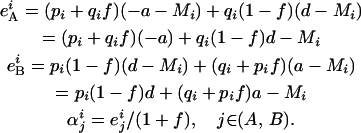(4)

Expression for the additive variance within population i is then

which, after replacement and simplifications gives

For a number n of populations, the expression becomes

(5)

From this expression we see that dominance decreases the additive variance within populations when the recessive allele is rare (p < 0.5), while it increases it when the recessive allele is frequent. This is easily understood since when the recessive allele is rare, it will be found mainly in heterozygotes that do not differ much in phenotype from the dominant homozygote.

The expression for Q_ST is obtained by replacing V_AW and V_B in Equation 1.

From Equations 3 and 5, we see that inbreeding diminishes the contribution of dominance to both V_B and V_AW. Thus, as inbreeding increases, the effect of dominance on Q_ST diminishes, and, unless , dominance will have little effect on Q_ST under strong inbreeding.

The expression of Q_ST for specific cases is listed below:

• No dominance, ∀f: In the absence of dominance (d = 0), V_AW reduces to

• while V_B takes the expression

• and Q_ST becomes

• Overdominance (no additivity), ∀f: When a = 0, expressions for V_B and V_AW become

• and

• and Q_ST becomes

• This is clearly very different from F_ST (Equation 2).

• f = 0: The expression for Q_ST does not simplify greatly when f = 0, as it remains a function of a, d, H_T, H_S, and p:

• f = 1: When f = 1, since the dominance term d comes as a product with (1 − f) in V_B and V_AW, it disappears altogether from their expressions and therefore also from that of Q_ST, as expected. Thus, .

As we have seen, the expression for Q_ST in the presence of dominance and inbreeding is not simple. To gain a better understanding of its effect, we start with a two populations system and first show contour plots for F_ST, Q_ST, and the difference (Q_ST − F_ST) for a trait encoded by one locus and two alleles as a function of the frequency of the recessive allele in two populations.

For a purely additive determinism, F_ST = Q_ST and the difference Q_ST − F_ST is therefore equal to zero for all points of the allele frequency space.

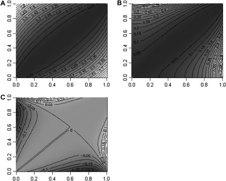
Figure 1 shows the contour plots for the case a = 1, d = 1, and f = 0. F_ST (Figure 1A) is null when the frequency is the same in the two populations and increases as allele frequencies diverge between the two populations, to reach a maximum of one when one allele is fixed in the first population and the other allele is fixed in the second.

Figure 1.

Contour plots of F_ST (A), Q_ST (B), and the difference Q_ST − F_ST (C) for two populations, as a function of the recessive allele frequencies in populations one (x-axis) and two (y-axis). The trait is dominant (additivity a and dominance d set to 1), and inbreeding is 0.

The contour plot for Q_ST is shown in Figure 1B. When the allele frequencies are the same in the two populations, Q_ST is null, as expected. The difference in allele frequencies when the recessive allele is rare in the two populations brings less changes in Q_ST than in F_ST. The effect of a difference in allele frequency increases as the recessive allele increases in frequency in both populations. When looking at the difference Q_ST − F_ST (Figure 1C) we observed that the difference is negative in the bottom left (when the recessive allele is rare in both populations), while it is positive in the top right (when the recessive allele is frequent). The negative area is larger than the positive one, and this is confirmed by integrating over the surface of allele frequencies: averaged over the allele frequency space, Q_ST = 0.162 while F_ST = 0.186. Thus, the expected difference between Q_ST and F_ST when there is dominance is negative.

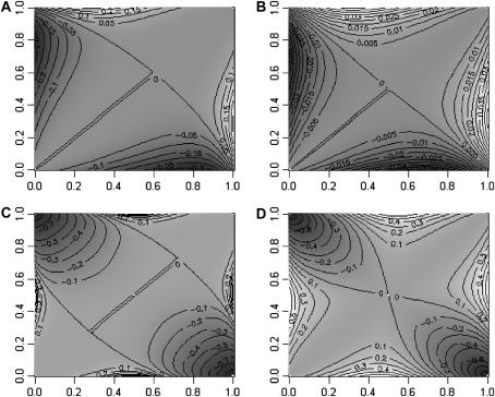
Figure 2 shows a contour plot of the difference between Q_ST and F_ST for different levels of dominance and inbreeding. Figure 2, A and B, represents the case a = 1, d = 1 seen in Figure 1. f = 0 for Figure 2A and this is therefore the same as for Figure 1C. In Figure 2B, f = 0.8, and we see that the difference between Q_ST and F_ST vanishes. It is 10-fold less than that with no inbreeding. And the mean value for Q_ST is now 0.185, very close to the average F_ST (= 0.186).

Figure 2.

Contour plots of the difference (Q_ST − F_ST) for two populations and different levels of dominance and inbreeding, as a function of the recessive allele frequencies in populations one (x-axis) and two (y-axis). (A and B) a = 1, d = 1, with f = 0 (A) and f = 0.8 (B). (C and D) Contour plots of Q_ST − F_ST but for an overdominant situation (a = 0, d = 1). (C) f = 0; (D) f = 0.8.

Figure 2, C and D, represents the case of strict overdominance (a = 0; d = 1). With strict overdominance and f = 0, a large area covering the secondary diagonal is negative (Figure 2C), and a much smaller portion of the contour plot has positive values for the difference. When integrating over the surface, the average Q_ST is 0.09. Therefore, with strict overdominance, Q_ST is on average much less than F_ST. With f = 0.8 (Figure 2D), the area where the difference between Q_ST and F_ST is negative reduces drastically while that where it is positive increases. And indeed, average Q_ST when f = 0.8 is 0.186, as is average F_ST. High inbreeding therefore cancels out the effect of overdominance on Q_ST.

Computer simulations:

With many loci and alleles, analytical results become intractable when there is dominance and inbreeding. We therefore used computer simulations to generate data under different levels of population structure, inbreeding, and trait determinism. Two types of simulations were used, one based on allele frequencies and the other on individuals.

Allelic frequencies:

First we drew allelic frequencies from Dirichlet distributions (Kingman 1977). Overall allelic frequencies [p] is a vector with its element obtained from a Dirichlet distribution of parameter 1, equivalent to a uniform distribution. To obtain frequencies at each locus in the different populations, a Dirichlet distribution with parameter 2Nm[p], where Nm is the number of migrants between populations, was used (Beaumont 2005).

From these allele frequencies, F_ST was obtained classically as , where . Similarly, H_T was estimated as , where p_jk is the realized overall allele frequency (i.e., it is not the original theoretical frequency [p] from the Dirichlet distribution). To account for bias due to the number of samples, (Nei 1987) was used instead of H_T in the expression of F_ST.

Traits were encoded by 10 10-allelic loci. Trait values were simulated by assigning to each allele at each locus an additive value drawn from a normal distribution. Similarly, to obtain a dominance effect of each genotype, a value drawn from a normal distribution was assigned to the dominance deviation of the genotype. The sum of the two additive effects and the dominance deviation gives the genotypic value of this genotype at the locus considered. Genotypic values for multilocus genotypes are obtained by summing the contributions of the individual loci, since we assume no epistasis. We also used exponential distributions instead of normal ones to draw additive value and dominance deviations, but this did not alter the results.

Once all these values are assigned, the within-population additive variance is estimated as (Lynch and Walsh 1998), with expressions for e_ij and α_ij given above (Equation 4); and the among-population variance of trait mean is simply that. Q_ST estimated this way is denoted Q_ST^p, where p stands for parent. Note that Q_ST^p cannot be estimated in experimental situations, as one would need allelic frequencies for all alleles contributing to the trait and the genotypic values for all genotypes.

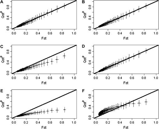
Figure 3 shows the relation between F_ST and Q_ST^p for pure additivity (Figure 3, A and B), dominance (Figure 3, C and D), and superdominance (Figure 3, E and F) under no inbreeding (Figure 3, A, C, and E) or strong inbreeding (f = 0.8; Figure 3, B, D, and F).

Figure 3.

Q_ST^p vs. F_ST for a trait coded by 10 10-allelic loci. Additive effects and dominance deviation are drawn from a normal distribution. (A–F) n = 10. (A, C, and E) f = 0; (B, D, and F) f = 0.8. (A and B) Purely additive trait; (C and D) dominant trait; (E and F) overdominant trait. Means are based on 100 replicates. F_ST and Q_ST^p are calculated as ratios of sums rather than the sums of ratios. Error bars represent ±1 standard deviation. The solid line is the line of equality between F_ST and Q_ST^p.

Under strict additivity, Q_ST^p = F_ST, as expected, and independently of the inbreeding coefficient. For traits with dominance and under random mating (Figure 3C), Q_ST becomes less than F_ST on average, and this tendency increases as populations get more structured. But this effect disappears in inbred populations (Figure 3D). With strict overdominance and under random mating (Figure 3E), the pattern observed with dominance is enhanced, and Q_ST^p is much lower than F_ST, the more so for very structured populations. With selfing and strict overdominance (Figure 3F), Q_ST^p is larger than F_ST for weakly structured populations, and smaller for those that are strongly structured.

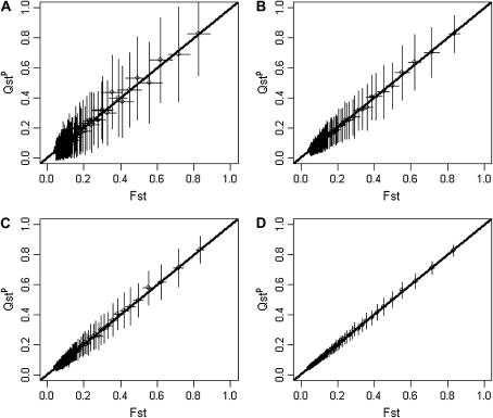
The results presented in Figure 3 are for simulations with 10 populations. The effect of the number of populations involved is presented in Figure 4, where only the situation with purely additive traits under random mating is presented. Figure 4 shows very clearly that the variance among replicates is huge with 2 populations (Figure 4A), still large with 5 populations (Figure 4B), and much smaller with 50 populations (Figure 4D).

Figure 4.

Q_ST^p vs. F_ST for a trait coded by 10 10-allelic loci. (A–D) Purely additive traits and no inbreeding. (A) n = 2; (B) n = 5; (C) n = 10; (D) n = 50. Means are based on 100 replicates. F_ST and Q_ST^p are calculated as ratios of sums rather than the sums of ratios. Error bars represent ±1 standard deviation. The solid line is the line of equality between F_ST and Q_ST^p.

Individual-based model:

The results just presented are for a theoretical situation where both allele frequencies at all loci involved in the trait and genotypic values for all genotypes are known, but this is never the case. When experimentalists estimate Q_ST, they use covariance among relatives to estimate additive variance rather than the allele frequencies at the loci underlying the trait, since these loci are generally unknown. To mimic this real situation we used an individual-based model with the following features:

We used Easypop (Balloux 2001) to generate genotypes from an individual-based finite island model, where islands exchange migrants at a fixed rate m, constant among populations and across generations. For all the simulations, population size N was fixed at 50 hermaphroditic individuals, and the number of populations n was also fixed at 50. For each individual, 100 loci with 20 allelic states each were simulated. The mutation rate was fixed at 0.001 and followed a K-allele model. Simulations were run for 500 generations, at which point F_ST had reached its equilibrium value for all levels of migrations. These were fixed at 0.002, 0.005, 0.01, 0.02, 0.05, 0.1, and 0.2, corresponding to Nm values of 0.1, 0.25, 0.5, 1, 2.5, 5, and 10, respectively. Two selfing rates were used, either 0 or 0.8. Genotypes of the last generation were stored for further processing.

Traits were encoded as in the simulations on allelic frequencies, by assigning additive values drawn from a normal distribution to each allele at each locus and dominance deviation to each genotype.

To estimate F_ST we used the genotypes at the trait loci of the parents and calculated F_ST using the method of Weir and Cockerham (1984) implemented in Fstat (Goudet 1995). To estimate Q_ST^o (where o stands for offspring), we proceeded as follows: A number of parents were chosen from each population of the island model. From these parents, a number of half-sib families (one male mated to 10 different females) were established, with 10 offspring each (1 offspring per female). We used either the full data set (10 individuals from 50 families from 50 populations, a total of 25,000 individuals) or subsamples of 1000 offspring from each data set, using the different sampling scenarios presented in Table 2.

TABLE 2.

Sampling designs used to infer Q_ST^o

Name	Populations	Families	Individuals
T	50	50	10
A	2	50	10
B	5	20	10
C	20	10	5
D	40	5	5

Sampling designs A–D consist of 1000 individuals in total.

These experimental sampling designs are similar to those used in several studies estimating Q_ST^o, with total number of individuals at 1000 (e.g., Spitze 1993; Lynch et al. 1999; Palo et al. 2003; Morgan et al. 2005). Often, however, the total number of individuals used to infer Q_ST is <1000 (e.g., Bonnin et al. 1996; Petit et al. 2001; Steinger et al. 2002).

A classical nested ANOVA was used to estimate the different variance components. V_AW is estimated as four time the among-family component of variance V_fam, while V_B is simply the among-population variance component.

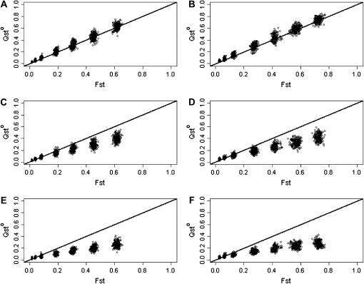
Figure 5 shows the relation between F_ST and Q_ST^o for additive (Figure 5, A and B), dominant (Figure 5, C and D), and superdominant (Figure 5, E and F) traits, for random mating (Figure 5, A, C, and E) and selfing (Figure 5, B, D, and F). For Figure 5, A–F, estimation of Q_ST^o is based on 50 families of 10 half-sibs from 50 populations. Under strict additivity (Figure 5, A and B), Q_ST^o = F_ST, and there is no difference between random mating and selfing populations. The observed pattern is congruent with that obtained for Q_ST^p (Figure 3, A and B).

Figure 5.

Q_ST^o as a function of F_ST for different trait determinisms and two levels of selfing. Estimation of Q_ST^o is based on 50 families of 10 half-sibs from 50 populations. Additive and dominance effects were drawn from a normal distribution. (A, C, and E) Random selfing; (B, D, and F) s = 0.8; (A and B) additive traits; (C and D) traits with both additivity and dominance; (E and F) overdominant traits.

For traits with dominance (Figure 5, C and D), Q_ST^o ≤ F_ST, and the difference increases as population structure increases. This is observed both for random mating and for selfing populations, and there seems to be very little difference in Q_ST^o between the two mating systems.

Finally, Figure 5, E and F, shows the effect of overdominance. Here, the pattern observed with dominance (Q_ST^o < F_ST, and the difference increasing with population structure) is amplified.

Effect of the crossing design:

We have seen that with allele frequency-based estimates of Q_ST, the effect of dominance on Q_ST^p disappears as selfing increases (Figure 3D), but when Q_ST is estimated with a half-sib design, the pattern Q_ST^o < F_ST remains (Figure 5D). However, the half-sib design is likely to unduly inflate additive variance estimates for a species that commonly selfs, and for strongly selfing species experimentalists often use selfed progeny to estimate the different genetic variance components and hence Q_ST (e.g., Bonnin et al. 1996; Steinger et al. 2002). With a selfed progeny design, additive variance cannot be singled out from dominance variance, but for a high selfer dominance variance is not naturally expressed as homozygous genotypes are transmitted intact to the next generation. With selfed progeny, Q_ST is estimated as , which amounts to assuming complete selfing (see Equation 1).

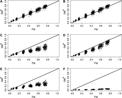
Using individual-based simulations with a high selfing rate (s = 0.889 f = 0.8), we compared estimates of Q_ST obtained from either half-sibs or selfed progenies. Figure 6 shows the results. Figure 6, A, C, and E, was obtained using a classical half-sib design, while Figure 6, B, D, and F, was obtained using a selfing design. With pure additivity (Figure 6, A and B), the two crossing designs give equivalent results. With dominance, estimates of Q_ST obtained from a selfed design (Figure 6D) are slightly less than but closer to F_ST than those obtained from a half-sib design (Figure 6C). This is particularly true for populations that are strongly structured. Hence, when the species under scrutiny is mainly selfing, estimates of Q_ST obtained from selfed progeny are less influenced by dominance, and thus preferable, to estimates obtained from a half-sib design. Another advantage of the selfing design is that it does not require a precise assessment of the inbreeding coefficient of the population (a prerequisite for the half-sib design).

Figure 6.

Effect of the crossing design used to infer Q_ST. (A–F) s = 0.889 (f = 0.8), and sampling is exhaustive. (A, C, and E) Variance components were estimated using a true half-sib design. For this design, Q_ST was estimated as . (B, D, and F) Variance components were estimated using 10 selfed offspring for each individual. For this design, Q_ST was estimated as . (A and B) Purely additive trait. (C and D) Dominant trait. (E and F) Overdominant trait (no additivity).

Last, Figure 6, E and F, shows the effect of the crossing design on traits that are purely overdominant. Figure 6E shows that under strict overdominance Q_ST is even less than under dominance when Q_ST is estimated from a half-sib design in a species with high selfing. If selfed progeny are used instead of half-sibs, Q_ST does not differ from zero whatever the level of population structure. This is expected, as under overdominance homozygote genotypes all have the same trait value. Selfed progeny from highly selfed parents are strongly homozygous in all populations, and therefore trait means are also identical among populations. Note that this is an artifact of having strict overdominance (i.e., the complete absence of additive effects).

Sampling strategies:

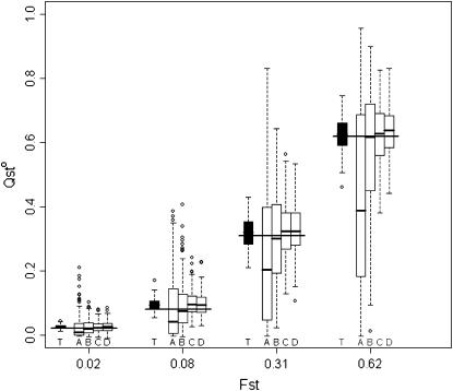
The effect of different sampling strategies on estimation of is shown in Figure 7. The box-plot representation gives a fair idea of the distribution of under these four sampling strategies. The worst scenario is strategy A (50 families of 10 individuals in two populations), which shows the largest variance for all levels of population differentiation and a negative bias that increases in magnitude as differentiation increases. Strategies C (20 populations) and D (40 populations) are best overall, with strategies C being slightly better for low structure and strategies D better for high structure. For scenarios C and D, the interquartile range is very similar to that under exhaustive sampling (Figure 7, labeled T).

Figure 7.

Effect of different sampling strategies on estimation for four different levels of population structure. The trait is purely additive and s = 0. For each of the four levels of population structure, the leftmost box-plot (labeled T) shows exhaustive sampling (50 half-sib families of 10 individuals from 50 populations). The other four sampling schemes are based on a total of 1000 individuals. From left to right, (A) 50 families of 10 individuals from 2 populations, (B) 20 families of 10 individuals from 5 populations, (C) 10 families of 5 individuals from 20 populations, and (D) 5 families of 5 individuals from 40 populations are shown. The long horizontal solid lines are drawn at the expected value of F_ST. Boxes correspond to the interquartile range and the short horizontal solid lines give the median of Q_ST.

DISCUSSION

While dominance can theoretically either increase or decrease Q_ST relative to its expectation under strict additivity, we have shown that, on average, dominance decreases the value of Q_ST, and the more differentiated the populations are, the stronger the effect. Thus, we conclude that dominance is unlikely to cause the pattern Q_ST > F_ST. Since this pattern was also shown to be unlikely under epistasis (Whitlock 1999; Lopez-Fanjul et al. 2003), we argue that when Q_ST > F_ST it is a good indicator of the presence of directional selection for different local optima. Q_ST < F_ST, on the other hand, could be the result of several factors other than homogenizing selection.

These results contrast with those obtained by Lopez-Fanjul et al. (2003), who found that the effect of dominance would more often increase Q_ST relative to F_ST rather than the reverse. There may be several reasons for this. First, Lopez-Fanjul et al. (2003) focused on populations that just underwent a severe bottleneck, and bottlenecks are known to alter (increase or decrease) the genetic variance both within and between lines (Robertson 1952; Willis and Orr 1993; Cheverud and Routman 1996; Naciri-Graven and Goudet 2003; Barton and Turelli 2004). Second, to compare F_ST and Q_ST, they did not use the allele frequencies at the loci coding for the trait as we did here, but used the expectation of the inbreeding coefficient among recently bottlenecked populations. Third, they looked at the effect of a one-generation bottleneck of two individuals, which would correspond to an F_ST of 0.25 on average, and did not investigate (as we did here) a range of population structure. Note that we also find situations in which Q_ST > F_ST, when the recessive allele is very common in most populations. But this situation is unlikely to be found frequently in nature, as recessive alleles are often deleterious, thus under the action of purifying selection, and therefore at low frequencies (Naciri-Graven and Goudet 2003; Barton and Turelli 2004).

In general, empirical studies tend to find Q_ST > F_ST (see reviews in Merila and Crnokrak 2001 and McKay and Latta 2002). Can we conclude from this pattern that directional selection is in action? Our results show that nonadditive gene actions are not the likely culprits, but other biases could produce this pattern.

Hendry (2002) pointed out that mutation is also likely to alter the relation between Q_ST and F_ST. The deflating effect of large mutation rate on F_ST is well known (Hedrick 1999; Balloux et al. 2000). If Q_ST is less sensitive to mutation than F_ST, or if the mutation rate at trait loci is smaller than at marker loci, then the mutation rate in itself can create the pattern expected under the action of directional selection. On the other hand, the mutation rate on a quantitative trait coded by several loci might be larger than that of one molecular marker. Thus, we concur with Hendry (2002): The potential effect of mutation rate on the relation between F_ST and Q_ST deserves a thorough investigation.

The large variance in Q_ST estimates based on few populations (and in many field situations, only a few populations are available) limits the statistical power of a test of the relation F_ST = Q_ST. O'Hara and Merila (2005) recently investigated the statistical properties of estimators of Q_ST and came to the same conclusion: With <12 populations, the variance in Q_ST is huge. We showed that this is particularly the case for very differentiated populations (F_ST > 0.2). With less differentiation, the problem seems less acute. We also showed that with few populations estimates of Q_ST seem to be biased downward. Thus, the pattern Q_ST > F_ST is unlikely due to a statistical artifact. Note that these arguments are only verbal, and more work is clearly necessary to refine the statistical tools available. In particular, our investigation of the effects of the sampling strategies needs to be pursued: We modeled traits that are purely genetically determined, and the effect of environmental variance on the precision of Q_ST estimates is not known, but is likely to inflate the variance of Q_ST.

It would be interesting to investigate the behavior of Q_ST under the joint action of selection and dominance. If the effect of dominance is just to hide recessive deleterious alleles, then recessive alleles will be rare and we saw that this is a situation where Q_ST < F_ST. Hence, the presence of deleterious recessive alleles should tend to make Q_ST even smaller than F_ST. If both purifying selection and directional selection for different optima are occurring, the deflating effect of dominance on Q_ST might cancel out the enhancing effect of directional selection. Hence, the pattern Q_ST = F_ST might reflect the joint action of these two selective forces rather than the absence of selection. A similar investigation on the effect of epistasis is also necessary.

Conclusions:

Despite these caveats and shortcomings, we have clearly shown that the pattern Q_ST > F_ST is unlikely for neutral traits with nonadditive gene action. Importantly, we have also shown that estimates of Q_ST are reliable only if based on many sampled populations. Providing that this is the case, the comparison between Q_ST and F_ST will remain useful in documenting the presence (or not) of local adaptation.

References

- Balloux, F., 2001. Easypop (version 1.7): a computer program for the simulation of population genetics. J. Hered. 92: 301–302. [DOI] [PubMed] [Google Scholar]
- Balloux, F., H. Brunner, N. Lugon-Moulin, J. Hausser and J. Goudet, 2000. Microsatellites can be misleading: an empirical and simulation study. Evolution 54(4): 1414–1422. [DOI] [PubMed] [Google Scholar]
- Barton, N. H., and M. Turelli, 2004. Effects of genetic drift on variance components under a general model of epistasis. Evolution 58(10): 2111–2132. [DOI] [PubMed] [Google Scholar]
- Beaumont, M. A., 2005. Adaptation and speciation: What can FST tell us? Trends Ecol. Evol. 20: 435–444. [DOI] [PubMed] [Google Scholar]
- Bonnin, I., J. M. Prosperi and I. Olivieri, 1996. Genetic markers and quantitative genetic variation in Medicago truncatula (Leguminosae): a comparative analysis of population structure. Genetics 143: 1795–1805. [DOI] [PMC free article] [PubMed] [Google Scholar]
- Cheverud, J. M., and E. J. Routman, 1996. Epistasis as a source of increased additive genetic variance at population bottlenecks. Evolution 50(3): 1042–1051. [DOI] [PubMed] [Google Scholar]
- Crnorkrak, P., and J. Merila, 2002. Genetic population divergence: markers and traits. Trends Ecol. Evol. 17: 501. [Google Scholar]
- Falconer, D., and T. MacKay, 1996. Introduction to Quantitative Genetics, Ed. 4. Prentice-Hall, Englewood Cliffs, NJ.
- Goudet, J., 1995. FSTAT (version 1.2): a computer program to calculate F-statistics. J. Hered. 86(6): 485–486. [Google Scholar]
- Hartl, D. L., and A. G. Clark, 1997. Principles of Population Genetics, Ed. 3. Sinauer Associates, Sunderland, MA.
- Hedrick, P. W., 1999. Highly variable loci and their interpretation in evolution and conservation. Evolution 53: 313–318. [DOI] [PubMed] [Google Scholar]
- Hendry, A., 2002. QST ≥=≠< FST? Trends Ecol. Evol. 17: 502. [Google Scholar]
- Kingman, J., 1977. Random discrete distributions. J. R. Stat. Soc. B 37: 1–22. [Google Scholar]
- Lande, R., 1992. Neutral theory of quantitative genetic variance in an island model with local extinction and recolonization. Evolution 46: 381–389. [DOI] [PubMed] [Google Scholar]
- Le Corre, V., and A. Kremer, 2003. Genetic variability at neutral markers, quantitative trait loci and trait in subdivided population under selection. Genetics 164: 1205–1219. [DOI] [PMC free article] [PubMed] [Google Scholar]
- Lopez-Fanjul, C., A. Fernandez and M. Toro, 2003. The effect of neutral nonadditive gene action on the quantitative index of population divergence. Genetics 164: 1627–1633. [DOI] [PMC free article] [PubMed] [Google Scholar]
- Lynch, M., and K. Spitze, 1994. Evolutionary genetics of Daphnia, pp. 109–128 in Ecological Genetics, edited by L. A. Real. Princeton University Press, Princeton, NJ.
- Lynch, M., and B. Walsh, 1998. Genetics and Analysis of Quantitative Traits, Ed. 1. Sinauer Associates, Sunderland, MA.
- Lynch, M., M. Pfrender, K. Spitze, N. Lehman, J. Hicks et al., 1999. The quantitative and molecular genetic architecture of a subdivided species. Evolution 53: 100–110. [DOI] [PubMed] [Google Scholar]
- McKay, J., and R. Latta, 2002. Adaptive population divergence: markers, QTL and traits. Trends Ecol. Evol. 17: 285–291. [Google Scholar]
- Merila, J., and P. Crnokrak, 2001. Comparison of genetic differentiation at marker loci and quantitative traits. J. Evol. Biol. 14: 892–903. [Google Scholar]
- Morgan, T. J., M. A. Evans, T. Garland, J. G. Swallow and P. A. Carter, 2005. Molecular and quantitative genetic divergence among populations of house mice with known evolutionary histories. Heredity 94: 518–525. [DOI] [PubMed] [Google Scholar]
- Naciri-Graven, Y., and J. Goudet, 2003. The additive genetic variance after bottlenecks is affected by the number of loci involved in epistatic interactions. Evolution 57(4): 706–716. [DOI] [PubMed] [Google Scholar]
- Nei, M., 1987. Molecular Evolutionary Genetics, Ed. 1. Columbia University Press, New York.
- O'Hara, R., and J. Merila, 2005. Bias and precision in QST estimates: problems and some solutions. Genetics 171: 1331–1339. [DOI] [PMC free article] [PubMed] [Google Scholar]
- Palo, J. U., R. B. O'Hara, A. T. Laugen, A. Laurila, C. R. Primmer et al., 2003. Latitudinal divergence of common frog Rana temporaria life history traits by natural selection: evidence from a comparison of molecular and quantitative genetic data. Mol. Ecol. 12: 1963–1978. [DOI] [PubMed] [Google Scholar]
- Petit, C., H. Freville, A. Mignot, B. Colas, M. Riba et al., 2001. Gene flow and local adaptation in two endemic plant species. Biol. Conserv. 100: 21–34. [Google Scholar]
- Pons, O., and K. Chaouche, 1995. Estimation, variance and optimal sampling of gene diversity. II. Diploid locus. Theor. Appl. Genet. 91: 122–130. [DOI] [PubMed] [Google Scholar]
- Pons, O., and R. Petit, 1995. Estimation, variance and optimal sampling of gene diversity. I. Haploid locus. Theor. Appl. Genet. 90: 462–470. [DOI] [PubMed] [Google Scholar]
- Robertson, A., 1952. The effect of inbreeding on the variation due to recessive genes. Genetics 37: 189–207. [DOI] [PMC free article] [PubMed] [Google Scholar]
- Rogers, A., and H. Harpending, 1983. Population structure and quantitative characters. Genetics 105: 985–1002. [DOI] [PMC free article] [PubMed] [Google Scholar]
- Spitze, K., 1993. Population structure in Daphnia obtusa: quantitative genetics and allozyme variation. Genetics 135: 367–374. [DOI] [PMC free article] [PubMed] [Google Scholar]
- Steinger, T., P. Haldimann, K. A. Leiss and H. Muller-Scharer, 2002. Does natural selection promote population divergence? A comparative analysis of population structure using amplified fragment length polymorphism markers and quantitative traits. Mol. Ecol. 11: 2583–2590. [DOI] [PubMed] [Google Scholar]
- Templeton, A., 1987. The general relationship between average effect and average excess. Genet. Res. 49: 69–70. [DOI] [PubMed] [Google Scholar]
- Weir, B., and C. Cockerham, 1984. Estimating F-statistics for the analysis of population structure. Evolution 38: 1358–1370. [DOI] [PubMed] [Google Scholar]
- Whitlock, M., 1999. Neutral additive variance in a metaopulation. Genet. Res. 74: 215–221. [DOI] [PubMed] [Google Scholar]
- Willis, J. H., and H. A. Orr, 1993. Increased heritable variation following population bottlenecks—the role of dominance. Evolution 47: 949–957. [DOI] [PubMed] [Google Scholar]
- Wright, S., 1951. The genetic structure of populations. Ann. Eugen. 15: 323–354. [DOI] [PubMed] [Google Scholar]
- Wright, S., 1969. Evolution and the Genetics of Populations. II. The Theory of Gene Frequencies, Vol. 2. University of Chicago Press, Chicago.
- Yang, R. C., F. C. Yeh and A. D. Yanchukt, 1996. A comparison of isozyme and quantitative genetic variation in Pinus contorta ssp. latifolia by FST. Genetics 142: 1045–1052. [DOI] [PMC free article] [PubMed] [Google Scholar]