Approximating Identity-by-Descent Matrices Using Multiple Haplotype Configurations on Pedigrees

Abstract

Identity-by-descent (IBD) matrix calculation is an important step in quantitative trait loci (QTL) analysis using variance component models. To calculate IBD matrices efficiently for large pedigrees with large numbers of loci, an approximation method based on the reconstruction of haplotype configurations for the pedigrees is proposed. The method uses a subset of haplotype configurations with high likelihoods identified by a haplotyping method. The new method is compared with a Markov chain Monte Carlo (MCMC) method (Loki) in terms of QTL mapping performance on simulated pedigrees. Both methods yield almost identical results for the estimation of QTL positions and variance parameters, while the new method is much more computationally efficient than the MCMC approach for large pedigrees and large numbers of loci. The proposed method is also compared with an exact method (Merlin) in small simulated pedigrees, where both methods produce nearly identical estimates of position-specific kinship coefficients. The new method can be used for fine mapping with joint linkage disequilibrium and linkage analysis, which improves the power and accuracy of QTL mapping.

IN statistical gene mapping by means of linkage and/or linkage disequilibrium (LD) analysis, the inheritance pattern of any specific chromosomal position in a pedigree can be captured by an identity-by-descent (IBD) matrix (Goring et al. 2003). The calculation of IBD matrices at putative quantitative trait loci (QTL) positions in pedigrees is an important step in statistical QTL mapping using variance component models. For the estimation of IBD matrices, hidden Markov methods are generally used on pedigrees of small to moderate size (Kruglyak and Lander 1995, 1998; Abecasis et al. 2002). For a complex pedigree, Wang et al. (1995) presented a recursive approach to estimate IBD probabilities, which utilizes only a single marker. Almasy and Blangero (1998) used a regression approach, where the IBD states at the markers are used to calculate IBD probabilities at a given locus. However, the regression coefficients used in the IBD calculation can be difficult to estimate in a complex pedigree.

For large pedigrees and large numbers of loci, Markov chain Monte Carlo (MCMC) methods (Sobel and Lange 1996; Thompson and Heath 1999; Sobel et al. 2001) were developed. However, MCMC methods can be very slow to converge, especially for data with dense markers, and convergence may be difficult to diagnose or may not be achieved (Pong-Wong et al. 2001). Pong-Wong et al. (2001) presented a deterministic method, which is fast on large pedigrees with multiple loci, but it uses only partially reconstructed haplotypes.

To calculate IBD matrices efficiently for large pedigrees and large numbers of loci, here we propose an approximation method using a set of haplotype configurations on a pedigree with high likelihoods, identified by a conditional enumeration haplotyping method (Gao et al. 2004; Gao and Hoeschele 2005). This method is compared with the MCMC method implemented in Loki (Heath 1997; Thompson and Heath 1999) based on QTL mapping performance in linkage analysis. The proposed method can incorporate LD information from historical recombinants, by allowing for nonzero IBD probabilities for founder alleles on the basis of the degree of similarity of the marker haplotypes surrounding the genome position in question (Meuwissen and Goddard 2000, 2001). In this article, we assume that all individuals in a pedigree have been genotyped for all markers. An extension to missing marker data is underway and will be reported in a subsequent contribution.

METHODS

Haplotype reconstruction:

In the space of all consistent haplotype configurations on a pedigree (SACHC), typically most configurations have very small probabilities so that only a relatively small subset of configurations is relevant. A consistent haplotype configuration is an assignment of haplotypes to all individuals in the pedigree, which is consistent with the observed genotype data and the pedigree structure. We previously presented a conditional enumeration haplotyping method based on conditional probabilities and likelihood computations to identify a subset of haplotype configurations with high conditional probabilities from SACHC (Gao et al. 2004; Gao and Hoeschele 2005). The conditional enumeration haplotyping method has been tested on published and simulated data sets and shown to be faster and provide more information than several existing stochastic and rule-based methods.

In a pedigree, the combination of a specific individual and a specific marker locus is termed a person-marker. The genotypes of some person-markers in nonfounders can be ordered by their parents' genotypes. Let U denote all remaining person-markers in a pedigree with unordered heterozygous genotype. Assume that the size of U is t. Reconstructing a haplotype configuration for the entire pedigree consists of assigning an ordered genotype to each person-marker in U. A set of t ordered genotypes assigned to the t person-markers in U is called a haplotype configuration for U.

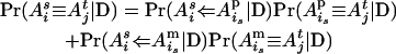
Let {M₁, M₂,…, M_t} be a specific order of the person-markers in U. Let m_i denote an ordered genotype assigned to person-marker M_i. The joint probability of a haplotype configuration for U, m₁, m₂,…, m_t, conditional on the observed data (D) is

(1)

Let . Also, m_i is one of the ordered genotypes and , where has the larger (smaller) conditional probability at person-marker M_i, and for j = 1, 2, with and . p_i is equal to one of the conditional probabilities and , so .

During haplotype reconstruction with the conditional enumeration method (Gao et al. 2004; Gao and Hoeschele 2005; see also the appendix), for some pedigrees that contain uninformative full- or half-sib families, at some person-marker , we find that , that is,

(2)

Hence the pedigree does not provide information to infer the phase at on the basis of , and D. When reconstructing a haplotype in an optimal reconstruction order , determined by the conditional enumeration method (Gao et al. 2004; Gao and Hoeschele 2005), if there are k person markers with (see Equation 2), let U_0.5 denote the set of these k person markers. If k is large (which happens only when a pedigree contains many uninformative full- or half-sib families), enumeration of all possible ordered genotype combinations at these k person-markers typically contributes little information to the IBD matrix estimation and to QTL mapping, but it increases the computing time substantially. Therefore, for IBD matrix calculation based on a limited number (say 2^s) of haplotype configurations with high likelihood and when s < k, then after enumerating two ordered genotypes for s person-markers in U_0.5 we adjust λ from its initial value (e.g., 0.90) down to 0.5, so that only a single, randomly chosen ordered genotype is assigned to each of the remaining k − s person-markers in U_0.5, where λ is a threshold for the conditional probabilities of ordered genotypes at each locus (λ ≥ 0.5; see Gao et al. 2004).

IBD matrix calculation:

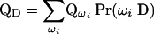
For a general pedigree, the IBD matrix at a specific genome location conditional on the observed data (D) is a weighted average of all IBD matrices, each conditional on a haplotype configuration in SACHC, where the weight of each configuration is the conditional probability of the configuration in SACHC. The IBD matrix conditional on the observed data (D) can be calculated by the expression

(3)

(Wang et al. 1995; Hoeschele 2003), where ω_i is a specific haplotype configuration of the pedigree in SACHC, Q_D () is the IBD matrix of the pedigree given D (ω_i), and Pr(ω_i|D) is the probability of ω_i conditional the observed data D. The summation in Equation 3 is over all configurations in SACHC.

For large pedigrees and large numbers of loci, it is infeasible to sum over all possible configurations in SACHC using Equation 3. Therefore, the exhaustive summation is approximated by the summation over a subset of haplotype configurations with high likelihoods identified by the conditional enumeration method. The probability Pr(ω_i|D) can be estimated approximately by the ratio of the likelihood of ω_i to the sum of the likelihoods of all configurations in the identified subset. Let n_s denote the size of the subset of haplotype configurations with high likelihoods identified by the conditional enumeration method and used to calculate IBD matrices.

For a specific haplotype configuration ω_i, the corresponding IBD matrix at a putative QTL position, , can be calculated by a deterministic, recursive method (Pong-Wong et al. 2001; Sobel et al. 2001). Suppose there are n individuals in a pedigree, identified with numbers 1, 2,…, n, so that parents always have smaller numbers than their offspring. Let denote the maternal (paternal) allele of individual i at the QTL position, and let denote the mother (s = m) or father (s = p) of i. The IBD probability between allele of individual i and allele of individual j at the QTL position conditional on observed data D is

(i > j, s = m, p and t = m, p) (Pong-Wong et al. 2001; Sobel et al. 2001), where, for example, is the probability that allele of individual i is inherited from the allele of its parent , and is the IBD probability between allele of parent and allele of individual j at the QTL position.

In linkage analysis, the IBD probabilities between the QTL alleles of any two founder haplotypes are assumed to be zero. For fine mapping using joint linkage disequilibrium and linkage analysis, linkage disequilibrium is incorporated via nonzero IBD probabilities for founder QTL alleles on the basis of the degree of similarity of the marker haplotypes surrounding the genome position in question. We currently compute these IBD probabilities by a gene-dropping method on a grid of putative QTL positions covering the entire genome or a chromosome region of interest (MacCluer et al. 1986; Meuwissen and Goddard 2000, 2001).

In the gene-dropping method, at any putative QTL position, it is assumed that a mutation occurred T_g generations before entering the founder generation of a pedigree and that the effective population size for the observed data is N_e. For each replicate of the simulation, T_g generations of an ancestral population are generated with N_e individuals and with the same marker positions as in the observed data. Let denote a haplotype pair that has a and b continuous identity-by-state (IBS) marker alleles between the QTL and the marker with the first non-IBS marker allele to the left and right of the QTL locus in the last generation (a ≥ 0, b ≥ 0) of any replicate, respectively. Let denote the total number of cases over 10,000 replications of the simulation, and let denote the number of cases that are IBD at the putative QTL. If two haplotypes are , the IBD probability at the QTL is

(4)

It is not easy to estimate T_g and N_e from the observed data. Meuwissen and Goddard (2000) performed a simulation, which showed that using values of T_g = 100 and N_e = 100, when the true values of these parameters varied, provided estimates of QTL position that were equally or even more accurate than the estimates obtained by using the true values of T_g and N_e. Therefore, we used the values of T_g = 100 and N_e = 100 in this study.

QTL mapping:

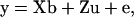
To evaluate the performance of the IBD matrix calculation method in QTL mapping, we use a two-step variance component method proposed by George et al. (2000) to estimate the QTL position and the variance parameters. When we assume a single QTL present at a specific genome position, in matrix notation, the phenotypic records of a pedigree can be modeled by

(5)

where y is a vector of phenotypes; b is a vector of fixed effects; u is a vector of random polygenic effects; v is a vector of random QTL effects; e is a vector of residuals; X and Z are known incidence/covariate matrices for the effects in b and in u and v, respectively; and u, v, and e are assumed to be uncorrelated. The variance-covariance matrix of the phenotypes under model (5) is

where A is the numerator relationship matrix; , and are variance components associated with vectors u, v, and e, respectively; , and ; and G = {g_ij} is the IBD matrix (for n individuals) at a specific QTL position conditional on the marker information, where

and, for example, is the IBD probability between the maternal allele of individual i and the paternal allele of individual j. In matrix notation (Van Arendonk et al. 1994), G = 0.5KQ_DK′, where K = I_n ⊗ [1, 1], ⊗ denotes the Kronecker product, and Q_D is the 2n × 2n gametic IBD matrix, which contains elements , where s = m, p; t = m, p; i = 1,…, n; and j = 1,…, n.

Assuming multivariate normality, or y ∼ N(Xb, V), the restricted log-likelihood of the data under model (5) can be represented as

(Patterson and Thompson 1971), where is the generalized least-squares estimator of b. When no QTL is assumed to be segregating in the pedigree, the mixed linear model (5) reduces to the null hypothesis model with no QTL, or

(6)

Given the IBD matrix G at a putative QTL position, parameters , and can be estimated by maximizing the restricted log-likelihood using ASReml (Gilmour et al. 2002) under models (5) and (6). Let L₁ and L₀ denote the maximized log-likelihoods pertaining to models (5) and (6), respectively.

To test the presence of a QTL (H₁) against no QTL (H₀) in a chromosomal region of interest, the test statistic log LR = −2(L₀ − L₁) is used. The asymptotic distribution of log LR under H₀ is not clear, because the null hypothesis places parameter on the boundary of its parameter space (Stram and Lee 1994; George et al. 2000). The distribution of log LR under H₀ is influenced by the chromosome segment length, the degree of missing marker data, and the distributional properties of the traits (George et al. 2000).

When testing a single marker interval in linkage analysis, Xu and Atchley (1995) and Grignola et al. (1996a,b) found that under H₀ the empirical distribution of log LR follows a χ²-distribution with degrees of freedom between 1 and 2 for independent full-sib families and related or unrelated half-sib families, respectively. For testing the presence of a QTL in a chromosomal region, George et al. (2000) reported that the empirical distribution of log LR was close to a -distribution for simulated pedigrees with 500 individuals. For simplicity and computational efficiency, in this study, we used the 5% critical values of both and to test for the presence of a QTL (H₁) against no QTL (H₀) in a chromosomal region of interest.

SIMULATION STUDY AND RESULTS

Comparison between our method and a MCMC method for estimating IBD matrices in linkage analysis:

Following George et al. (2000), we used a two-step variance components method to perform QTL linkage analysis for 50 simulated pedigrees based on the ASReml software (Gilmour et al. 2002). We computed IBD matrices at each putative QTL position with our method as described above and with the MCMC method implemented in Loki (Heath 1997; Thompson and Heath 1999), assuming zero IBD probabilities between any two founder QTL alleles. The calculation of IBD matrices with Loki and the subsequent variance components linkage analysis with ASReml for pedigrees have been extensively described and tested by George et al. (2000).

Simulation of pedigree data for linkage analysis:

Each simulated pedigree contained 33 founders (11 fathers and 22 mothers) and seven generations of nonfounders. Founder marker haplotypes were generated assuming Hardy-Weinberg equilibrium at each locus and linkage equilibrium between loci. Haplotypes for nonfounders were simulated conditional on their parental haplotypes, assuming Haldane's no interference mapping function. The chromosomal region consisted of ten biallelic markers with allele frequency of 0.5 and distance between adjacent markers of 5 cM. A biallelic QTL with allele frequency of 0.5 was located at position 22.5 cM (the midpoint between markers 5 and 6), and the QTL was additive and explained 10% of the trait variance. Each father had two spouses, and each full-sib family had three children. The size of the pedigrees ranged from 470 to 500. A total of 50 pedigrees were simulated. A set of 27 putative QTL positions (not at marker loci) was chosen across the chromosomal region of interest (see below).

Assuming no fixed effects, the phenotype of individual i was generated as

(7)

where u_i, v_i, and e_i were the polygenic effect, QTL effect, and residual of individual i, respectively. For founders, u_i was drawn from the normal distribution , and for nonfounders, u_i was drawn from a normal distribution with mean 0.5(u_f + u_m) and variance 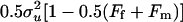, where u_f and u_m are the polygenic effects and F_f and F_m the inbreeding coefficients of the father and mother of i, respectively. If individual i had genotype QQ, Qq, or qq at the QTL, v_i was set equal to a, 0, or −a, respectively. QTL variance was 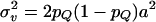, and p_Q was the Q-allele frequency (Falconer and Mackay 1996; George et al. 2000). Residuals were drawn from . Parameter values were , and .

Results for linkage analysis:

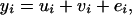
Figure 1 presents the average log LR profiles over the 50 replicated pedigrees, using IBD matrices calculated by Loki (100,000 iterations) and by our method with two sets of values for control parameters λ, α, and n_s (the size of the subset of haplotype configurations with high likelihoods used to calculate IBD matrices). Figure 1 shows that the three profiles are nearly identical.

Figure 1.

Average test statistic (log LR) profiles over 50 replicated pedigrees of size 470–500, with 10 biallelic markers, intermarker distance of 5 cM, true QTL position at 22.5 cM, and QTL variance at 10% of the trait variance. IBD matrices were calculated in three ways: “New1” and “New2,” which denote the proposed method with λ = 0.65, α = −0.3, and n_s = 50 and with λ = 0.90, α = −1.0, and n_s = 50, respectively, and “Loki,” which represents use of the Loki software with 100,000 iterations. See main text for explanation of control parameters λ, α, and n_s.

For each of the 50 pedigrees, we estimated the QTL position as the location with the highest log-likelihood among all 27 putative positions under model (5). Estimates of the variance components were the values maximizing the log-likelihood at this chosen QTL position. Table 1 presents means, standard deviations (SD), and mean-square errors (MSE) of the parameter estimates over 50 pedigrees using IBD matrices calculated by Loki and our method with the two sets of control parameter values (λ = 0.65, α = −0.3, and n_s = 50; λ = 0.90, α = −1.0, and n_s = 50). Table 1 shows that means, SD, and MSE of the estimates of QTL position () and variance parameters 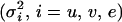obtained with Loki and our method are very similar, with the estimates from our method being very slightly closer to the true values than those from Loki. Using our method with the second set of control parameter values (λ = 0.90, α = −1.0, and n_s = 50) produced slightly smaller SD and MSE, except for the estimate of . Among the 50 replicated pedigrees, in 8 replicates our method provided more accurate estimates of QTL position compared with Loki, and in 5 (4) replicates, our method with control parameter set 1 (2) provided less accurate estimates.

TABLE 1.

Parameter estimates obtained using Loki and the method proposed here for IBD matrix calculation based on 50 replicated pedigrees

Parametersa	True value	Methodb	Mean estimate	SDc	MSEd
	2.0	New1	1.9777	0.5800	0.3301
New2	1.9789	0.5795	0.3295
Loki	1.9648	0.5788	0.3296
	0.5	New1	0.5774	0.2541	0.0693
New2	0.5770	0.2541	0.0692
Loki	0.5839	0.2576	0.0721
	2.5	New1	2.5288	0.2795	0.0774
New2	2.5284	0.2786	0.0769
Loki	2.5325	0.2810	0.0785
	22.5	New1	21.750	8.493	0.7125
New2	21.825	8.066	0.6422
Loki	21.425	8.364	0.6972
Log LR	—	New1	10.2872	5.8044	—
New2	10.2930	5.8038	—
		Loki	10.3230	5.8704	—

^aParameters from top to bottom are polygenic, QTL, and residual variance; QTL position; and test statistic.

^bNew1 (New2) denotes using the proposed method with λ = 0.65, α = −0.3, and n_s = 50 (λ = 0.90, α = −1.0, and n_s = 50); see main text for explanation of these control parameters.

^cStandard deviation of the estimates over 50 replicates.

^dMean square error of the estimates over 50 replicates.

While the parameter estimates obtained with Loki and our method are very similar (Table 1), and profiles obtained with the two methods are nearly identical (Figure 1), the proposed method uses much less computing time than Loki in calculating IBD matrices. Table 2 presents the computing times of both methods for calculation of IBD matrices at the 27 putative QTL positions on a workstation with 2.00 GHz Intel Xeon CPU (1,047,546 kB RAM; Linux kernel 2.4.22).

TABLE 2.

Computing times for calculation of IBD matrices at 27 QTL positions for pedigrees of size 470–500 with Loki and the proposed method

				Computing time (hr:min:sec)
Methoda	λ	α	ns	Mean	SD
New1	0.65	−0.3	50	0:5:16	0:1:2
New2	0.90	−1.0	50	0:25:7	0:29:37
Loki	—	—	—	1:46:0	0:3:5

^aNew1 (New2) denotes using the proposed method with λ = 0.65, α = −0.3, and n_s = 50 (λ = 0.90, α = −1.0, and n_s = 50).

To compare the power of QTL detection using our method and Loki, we tested for a single QTL in the chromosomal region of interest using the 5% critical values of the chi-square distributions with 1 and 2 d.f., 3.84 and 5.99. It is obvious from Figure 1 that there is essentially no difference in power between the two methods, but more detailed results are in Table 3. Table 3 shows that the numbers of replicates with a type II error (null hypothesis H₀ of no QTL not rejected), or with QTL identification in the kth marker intervals to the left or right of the true interval (k = 0, 1,…, 4), are essentially the same for both methods.

TABLE 3.

Power and accuracy of QTL detection in a chromosomal region using threshold values from chi-square distributions with 1 d.f. (3.84) and 2 d.f. (5.99), with IBD matrix calculation by the method proposed here (with n_s = 50) and by Loki based on analysis of 50 pedigrees

				No. of replicates with estimated position in the kth interval to the left or right of the true intervala					No. of replicates not rejecting H0b
Critical value	Method	λ	α	0	1	2	3	4
3.84	Loki	—	—	17	12	3	6	3	9
New1	0.65	−0.3	18	10	3	7	3	9
New2	0.90	−1.0	18	10	4	7	2	9
5.99	Loki	—	—	16	11	3	6	2	12
New1	0.65	−0.3	16	9	3	7	3	12
	New2	0.90	−1.0	16	9	4	7	2	12

^aNumber of replicates with estimated QTL position in the kth interval to the left or right of the true interval and with log LR larger than the critical value (k = 0, 1,…, 4); k = 0 denotes that the estimated position is in the same interval as the true position.

^bNumber of replicates with log LR less than or equal to the critical value, where assuming H₀: no QTL is present in the chromosomal region.

Linkage analysis of a single, larger pedigree with a larger number of linked loci:

We simulated a pedigree of 1024 individuals and 50 linked biallelic markers with allele frequency of 0.5 and intermarker distance of 1 cM. The pedigree had 60 founders (20 fathers and 40 mothers) and 16 generations of nonfounders. A biallelic QTL with allele frequency of 0.5 was located at position 24.5 cM (the midpoint between markers 25 and 26), and the QTL was additive and explained ∼18% of the trait variance. Each father had two spouses, and each full-sib family had two children. The phenotypic data were simulated as described earlier.

We calculated IBD matrices at 49 putative QTL positions (midpoints of the marker intervals) using the proposed method and Loki. Using the proposed method with λ = 0.65, α = −0.3, and n_s = 50, we obtained nonsingular IBD matrices at the 49 positions with computing time of 39 min and 34 sec. Figure 2 presents the corresponding log LR profile, which has a peak at 25.5 cM, 1 cM away from the true QTL position.

Figure 2.

Test statistic (log LR) profile for a pedigree of 1024 individuals, with 50 biallelic markers, intermarker distance of 1 cM, true QTL position at 24.5 cM, and QTL variance at 18% of the trait variance. IBD matrices were calculated with the proposed method using control parameter values of λ = 0.65, α = −0.3, and n_s = 50.

Estimation of the IBD matrices by using Loki with 100,000 iterations took 22 hr, 4 min, and 34 sec. However, all estimated IBD matrices were either singular or very close to singular and hence could not be inverted. Although singular matrices can be used for QTL mapping by the method of Visscher et al. (1999), it is preferable to obtain nonsingular estimates of IBD matrices if possible on the basis of the observed data, because in our experience the singular estimates often result from executing Loki with an insufficient number of iterations, and increasing the number of iterations can lead to nonsingular estimates. However, for very large pedigrees with large numbers of linked loci a sufficient increase in the number of iterations with Loki may not be computationally feasible.

Effect of the control parameters of the haplotyping algorithm on QTL mapping accuracy:

The results presented in Table 1 for our proposed method (New1 and New2) indicate that for the ∼500-member pedigrees a change in the settings of control parameters λ and α from 0.65 and −0.3 to 0.90 and −1.0 slightly improves the accuracy of the estimates of parameters (QTL position and variance parameters), for a given setting of . To further investigate the influence of different values of on the parameter estimates and the likelihood ratios, we compared two settings of (50 and 1000) under two combinations of λ and α. This comparison was performed on selected pedigrees to limit computing time. As an example, Table 4 presents parameter estimates obtained with different values of λ, α, and for a single pedigree of 483 individuals from the set of 50 replicated pedigrees described earlier, and Figure 3 presents the corresponding log LR profiles for this pedigree.

TABLE 4.

Parameter estimates obtained using the proposed IBD matrix method with different values of control parameters λ, α and n_s from linkage analysis of a single 483-member pedigree

			Estimatesa
λ	α	ns					Log LR	Time (hr:min:sec)
0.65	−0.3	50	2.0040	0.5873	2.7650	21.25	10.908	0:5:46
1000	2.0041	0.5874	2.7648	21.25	10.910	1:18:0
0.90	−1.0	50	2.0044	0.5871	2.7648	21.25	10.906	0:23:3
		1000	2.0041	0.5874	2.7648	21.25	10.910	5:8:37

^aEstimates from left to right are of polygenic, QTL, and residual variance; QTL position; and test statistic.

Figure 3.

Test statistic (log LR) profiles obtained using the new IBD matrix calculation method with different values of control parameters λ, α, and n_s for a single pedigree. The pedigree had 483 individuals with 10 biallelic markers, true QTL position at 22.5 cM, and intermarker distance of 5 cM. A denotes the profile of log LR with λ = 0.65, α = −0.3, and n_s = 50; B, the profile with λ = 0.65, α = −0.3, and n_s = 1000; C, the profile with λ = 0.90, α = −1.0, and n_s = 50; and D, the profile with λ = 0.90, α = −1.0, and n_s = 1000.

Table 4 shows that for both sets of values for λ and α, increasing n_s from 50 to 1000 produces essentially the same parameter estimates and likelihood ratios. In addition, for the same n_s value, there is essentially no difference in parameter estimates and likelihood ratios for the two combinations of values of λ and α. However, increasing either n_s or the absolute values of λ and α causes very substantial increases in computing time. Figure 3 also shows that the log LR profiles are almost identical for the four sets of values of λ, α, and n_s. Similar results (not shown) were found for almost all of other simulated pedigrees.

Comparison between our method and an exact method for estimating IBD probabilities in small pedigrees:

To evaluate the performance of the new method for small pedigrees, we simulated 20 replicated pedigrees. Each pedigree has 15 individuals (including three founders, one father and two mothers) spanning four generations and 10 linked biallelic markers with allele frequency of 0.5 and intermarker distance of 1 cM. On average, each father had two spouses, and each full-sib family had two children. Let K(i, j) denote the position-specific kinship coefficient between individual i and j, at a putative QTL position, or

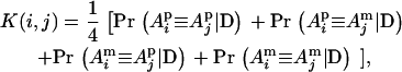where, for example, is the IBD probability between the maternal allele of individual i and the paternal allele of individual j. We computed kinship coefficients at nine putative QTL positions (midpoints of the marker intervals) with our method as described above (λ = 0.999, α = −3.2) and with the exact method implemented in Merlin (Abecasis et al. 2002), assuming zero IBD probabilities between any two founder QTL alleles. Let D(i, j) denote the absolute difference between the two estimates of K(i, j) using our new method and Merlin. The largest value of D(i, j) over all pairs of individuals, all nine putative positions, and 20 replicates is 0.008969. So both methods have nearly identical estimates for each K(i, j). The average value of all nonzero D(i, j) is 0.00034975. The computing times are 34 ± 94 and 66 ± 23 sec for the new method and Merlin, respectively.

IBD matrix calculation with linkage disequilibrium:

In joint linkage and linkage disequilibrium mapping, for each of the n_s haplotype configurations with high likelihoods used for IBD matrix calculation, the IBD submatrix of the founder haplotypes was calculated using the gene-dropping method (Meuwissen and Goddard 2000), the IBD submatrices pertaining to founders and descendants and for descendants were calculated by the recursive method (Pong-Wong et al. 2001; Sobel et al. 2001), and the weighted average of the n_s IBD matrices was obtained as described earlier. Here we used only our proposed method for IBD matrix calculation, because Loki does not incorporate nonzero IBD probability values among founder haplotypes. To evaluate the performance of the proposed IBD matrix method in joint linkage and linkage disequilibrium mapping and the influence of different values of λ, α, and on the estimated results, we analyzed 50 simulated, replicated pedigrees with linkage disequilibrium.

Simulation of pedigrees with linkage disequilibrium:

We assumed that a mutation happened 100 generations before entering each pedigree. We simulated 100 generations of an ancestral population as in Meuwissen and Goddard (2000). Each generation had an effective size of 100 with 50 males and 50 females. The simulated chromosomal region contained 20 biallelic markers with intermarker distance 1 cM and a biallelic QTL located halfway (9.5 cM) between markers 10 and 11. In the first ancestral generation, the two alleles of each marker locus were sampled according to allele frequencies 0.5, and each of the 200 QTL alleles was assigned a unique number. For each of the subsequent ancestral generations, each of 50 males and 50 females was produced by randomly sampling parents from the previous generation. Among the QTL alleles that were still present in the last (100th) generation, the allele with a frequency near the desired value of 0.15 was chosen to be the mutant allele (Q), while all other QTL alleles were assumed to be wild type (q).

For each pedigree, the founder generation (14 males and 28 females) was randomly sampled from the latest (100th) generation of the ancestral population. Nine descendant generations were generated, with parents randomly sampled from the previous generation. Pedigree size ranged from 480 to 510, with each father having two spouses and each full-sib family having two children. Phenotypes were simulated as described earlier, and the QTL explained 10% of the trait variance. Fifty pedigrees were generated.

Results for joint linkage and linkage disequilibrium mapping:

IBD matrices were calculated at 19 putative QTL positions (midpoints of the 19 marker intervals). Figure 4 presents the average log LR profiles over the 50 replicated pedigrees, using the proposed IBD matrix calculation method with three sets of values for control parameters λ, α, and when incorporating linkage disequilibrium. Figure 4 shows that when λ and α changed from 0.65 and −0.3 to 0.90 and −1.0, and increased from 50 to 1000, the average log LR profile remained essentially unchanged, and each of the average log LR profiles has its peak at the true QTL position of 9.5 cM.

Figure 4.

Average test statistic (log LR) profiles over 50 replicated pedigrees of size 480–510, with 20 biallelic markers, intermarker distance of 1 cM, true (biallelic) QTL position at 9.5 cM, and QTL variance at 10% of the trait variance. IBD matrices were calculated with the proposed method incorporating linkage disequilibrium. New1 denotes the new IBD matrix method with λ = 0.65, α = −0.3, and n_s = 50; New2 has λ = 0.90, α = −1.0, and n_s = 50; and New3 has λ = 0.90, α = −1.0, and n_s = 1000.

Table 5 presents the parameter estimates produced with the new IBD matrix calculation method for different values of λ, α, and , when incorporating LD in the analysis of the 50 replicated pedigrees. Table 5 shows that when the values of λ and α change from 0.65 and −0.3 to 0.90 and −1.0, and when increases from 50 to 1000, mean, SD, and MSE of all parameters are not notably affected. For all sets of values for λ, α, and , the parameter estimates were generally close to the true values except for , which was overestimated. This overestimation was also reported by Grignola et al. (1996b) and George et al. (2000).

TABLE 5.

Parameter estimates produced with the proposed IBD matrix calculation method when incorporating LD in the analysis of 50 pedigrees and for different values of the control parameters λ, α, and n_s

Parametersa	True value	λ	α	ns	Mean estimate	SDb	MSEc
	1.02	0.65	−0.3	50	1.0541	0.2255	0.0510
0.90	−1.0	50	1.0535	0.2257	0.0510
0.90	−1.0	1000	1.0521	0.2270	0.0515
	0.255	0.65	−0.3	50	0.3994	0.2295	0.0725
0.90	−1.0	50	0.4002	0.2297	0.0727
0.90	−1.0	1000	0.4017	0.2306	0.0736
	1.275	0.65	−0.3	50	1.2855	0.1451	0.0207
0.90	−1.0	50	1.2856	0.1451	0.0208
0.90	−1.0	1000	1.2861	0.1453	0.0208
	9.5	0.65	−0.3	50	9.68	2.3707	0.0554
0.90	−1.0	50	9.68	2.3707	0.0554
0.90	−1.0	1000	9.62	2.3355	0.0536
Log LR	—	0.65	−0.3	50	19.6072	12.4949	—
0.90	−1.0	50	19.6382	12.5213	—
		0.90	−1.0	1000	19.7072	12.6154	—

^aParameters from top to bottom are polygenic, QTL, and residual variance; QTL position; and test statistic.

^bStandard deviation of the estimates over 50 replicates.

^cMean square error of the estimates over 50 replicates.

To evaluate the power of joint LD and linkage mapping using the proposed IBD matrix calculation method for different values of control parameters λ, α, and n_s, tests were conducted for the presence of a single QTL (H₁) vs. no QTL (H₀) in the chromosomal region of interest, using the 5% critical values of the - and -distributions, 3.84 and 5.99. Table 6 presents the test results from the analysis of the 50 replicated pedigrees. Table 6 shows that when calculating the IBD matrices with control parameter settings “New1” (λ = 0.65, α = −0.3, and n_s = 50) and “New2” (λ = 0.90, α = −1.0, and n_s = 50), the results are identical and very similar to those obtained with “New3” (λ = 0.90, α = −1.0, and n_s = 1000). For New1 or New2, with critical value 3.84 (5.99), among the 50 replicates, 44 (40) were found to have a QTL in the chromosomal region, and 34 (30) had the estimated QTL position in the correct marker interval or in the left or right adjacent interval. Similar results can be found for New3.

TABLE 6.

Power and accuracy of QTL detection in a chromosomal region of interest using threshold values from chi-square distributions with 1 d.f. (3.84) and 2 d.f. (5.99), obtained with the proposed method for IBD matrix calculation when incorporating LD in the analysis of 50 pedigrees

		No. of replicates with estimated position in the kth interval to the left or right of the correct intervalb										No. of replicates not rejecting H0c
Critical value	Methoda	0	1	2	3	4	5	6	7	8	9
3.84	New1/New2	20	14	4	3	0	2	0	1	0	0	6
New3	21	14	4	2	0	2	0	1	0	0	6
5.99	New1/New2	20	10	4	3	0	2	0	1	0	0	10
	New3	21	10	4	2	0	2	0	1	0	0	10

^aNew1 denotes the new IBD matrix calculation method with control parameter settings λ = 0.65, α = −0.3, and n_s = 50; New2 has λ = 0.90, α = −1.0, and n_s = 50; New3 has λ = 0.90, α = −1.0, and n_s = 1000. New1/New2 denotes that New1 and New2 gave the same results.

^bNumber of replicates with log LR larger than the critical value (H₀ was rejected) and with estimated QTL position in the kth marker interval to the left or right of the true interval (k = 0, 1,…, 4), where k = 0 denotes an estimated position in the correct marker interval.

^cNumber of replicates with log LR less than or equal to the critical value, when assuming H₀: no QTL is present in the chromosomal region.

The accuracy of QTL identification and estimation achieved with the incorporation of linkage disequilibrium for variance component analysis has been investigated by Meuwissen and Goddard (2000). Here our goal is to show that their approach for IBD matrix calculation in founders, which assumes known marker haplotypes, can be easily combined with our conditional enumeration method for haplotype reconstruction. The proposed method for calculation of IBD matrices incorporates LD and is applicable to the realistic situation of marker haplotype uncertainty in pedigree data.

DISCUSSION

As genetic marker maps continue to become denser and more precise, there is an increasing demand for multipoint QTL analysis of large and complex pedigrees. Exact computations become infeasible, necessitating the use of approximation methods (Thompson and Heath 1999). The proposed new IBD matrix calculation method is shown to be an efficient approach applicable to larger pedigrees and larger numbers of linked loci than other available methods, while at least maintaining the same QTL mapping accuracy as the MCMC method implemented in Loki. It is based on a conditional enumeration haplotyping method (Gao et al. 2004; Gao and Hoeschele 2005), which is more efficient for densely linked markers. The new IBD matrix calculation method uses a subset of haplotype configurations with high likelihoods identified by the enumeration method. It does not have the mixing problem, which often exists in MCMC methods, in particular for very tight linkage (Thompson and Heath 1999).

The proposed method uses only the informative markers for the individual under consideration and its parents and offspring according to optimal reconstruction orders for the pedigree (Gao et al. 2004; Gao and Hoeschele 2005) and is hence not affected by the presence of loops in the pedigree.

When increasing the average relationship/inbreeding coefficient of the pedigree, the sizes of full-sib or half-sib families, the number of linked loci, or the number of alleles per marker locus, the pedigree becomes more informative, and the subset of haplotype configurations with highest likelihoods accounts for a larger percentage of the total probability, this increasing the efficiency of our haplotyping and IBD matrix calculation methods.

The computing time of the new method can be controlled by the values of two threshold parameters (λ and α, which affect the number of enumerated configurations) and the size of the retained subset of haplotype configurations used for IBD matrix calculation, n_s. Given a set of values for control parameters λ, α, and n_s, the computing time of the proposed method depends on how informative the pedigree is. For an IBD matrix at a putative QTL position, the computing time does not always increase much or at all when the number of linked loci or the size of the pedigree increases, because of the larger amount of information in the full- and half-sib families of the pedigree.

In our simulation studies, we found that the estimates of QTL position and variance components obtained by the proposed IBD matrix calculation method change very little with changes in the settings of the control parameters λ, α, and n_s (n_s ≥ 50). For the types of pedigrees that we simulated (full-sib families with two or three children, each father having two spouses, and biallelic marker loci), increasing n_s beyond the value of 50, while leaving λ and α constant, did not notably change the estimates of QTL position and variance components; for the same value of n_s, increasing the absolute values of λ and α at most slightly improved estimation accuracy, but at the cost of a substantial increase in computing time. This robustness of the estimates is expected to be true for general pedigrees, in particular for more informative pedigree structures with larger full- or half-sib families, more spouses per parent, larger numbers of linked loci, or more alleles per locus. Consequently, analysis of quite large pedigrees with large numbers of dense markers should be feasible by selecting settings of the control parameters λ, α, and n_s with low absolute values that provide computational efficiency while maintaining sufficient power and accuracy of QTL inference. It is advisable to run a QTL analysis with at least two different settings of the control parameters to verify robustness in each application.

In the linkage analysis of simulated pedigrees with intermarker distance of 5 cM (Figure 1, Table 1), when λ, α, and n_s had low absolute values (λ = 0.65, α = −0.3, and n_s =50), i.e., values yielding high computational efficiency, the estimates and their accuracies obtained with our proposed method were essentially identical to those obtained by computing the IBD matrix with the MCMC algorithm implemented in Loki (100,000 iterations), while the computing time of the new method was much shorter (see Table 2).

Pong-Wong et al. (2001) compared their deterministic method with Loki via their performance in linkage analysis of simulated replicates of pedigree data. This deterministic method used only partially reconstructed haplotypes for each individual. Although the shape of average log LR profiles over simulated replicates was similar for both methods, the average values of log LR from the deterministic method were lower than those using Loki at putative QTL positions close to the true position and higher than those using Loki at some positions far from the true position (Pong-Wong et al. 2001). In contrast, in our simulation study, our new method and Loki always have essentially identical average values of log LR at all putative QTL positions.

Using the MCMC method in Loki, if the number of iterations is too small, then it is more likely that the estimates of the IBD matrices will be singular. When the pedigree size or the number of linked markers increases, more iterations are often needed to avoid obtaining too many singular IBD matrices. The MCMC method may therefore become computationally infeasible for large pedigrees and large numbers of linked loci.

When intermarker distances are 1 cM or less and for pedigrees that are not very informative (i.e., lack sufficient numbers of recombination events), the estimates of the IBD matrices at some putative QTL positions may be singular (not often). Increasing the number of linked loci may decrease the probability of obtaining a singular IBD matrix. In addition, the IBD matrices at marker loci may be singular (George et al. 2000). In this study, putative QTL positions were chosen not to coincide with marker locations. For the singular IBD matrices, an algorithm not requiring inversion of the IBD matrices can be used for restricted maximum likelihood (REML) estimation (Visscher et al. 1999; George et al. 2000); however, this algorithm is always computationally more intensive than algorithms using inverses of IBD matrices, such as the algorithm implemented in ASReml.

In the proposed method an IBD matrix is estimated by a weighed average of IBD matrices conditional on a subset of haplotype configurations with high likelihoods, while in the MCMC method in Loki it is estimated by an arithmetic average of IBD matrices conditional on a set of inheritance vectors or sets of segregation indicators (Thompson and Heath 1999). For the situation investigated here with unordered genotypes known for each individual and all marker loci (no missing data case), the size of the subset of configurations in the proposed method can be quite small (50 for pedigrees with 500–1000 individuals) without compromising QTL mapping accuracy. Because of homozygous genotypes in the pedigree, a haplotype configuration is often consistent with and then contains all information in multiple inheritance vectors or sets of segregation indicators used by the MCMC method in Loki. This might be one of the reasons why the proposed method using a subset of as little as 50 haplotype configurations produces QTL mapping results that are essentially identical to those obtained by computing the IBD matrix using the MCMC algorithm in Loki with 100,000 iterations.

In this study, we assumed that all individuals in a pedigree were genotypes at all markers. Work is underway to extend our method to situations with substantial amounts of missing marker data.

The IBD matrix calculation method presented in this article was implemented in a C++ program, which is available upon request from the first author for academic research.

APPENDIX: A CONDITIONAL ENUMERATION METHOD FOR HAPLOTYPING IN PEDIGREES

In Equation 1, calculating the conditional probabilities () using all the available information in a large pedigree is computationally infeasible. We therefore use only the informative flanking marker information of a locus under consideration from the corresponding individual and its close relatives: parents and offspring (Gao et al. 2004). From Equation 1, the conditional probability of the haplotype configuration can be written as

Let T denote the largest conditional probability of all haplotype configurations for U, and let R denote the ratio of the conditional probability of haplotype configuration to T. For any , let . Because , and is very likely true (see Gao and Hoeschele 2005 for details), the following inequality is very likely to hold:

(A1)

Given a relatively small threshold , if we can find some , such that , then from inequality (A1) we have , so the conditional probability is very small relative to the largest conditional probability T. Then this configuration can be deleted from SACHC, when the purpose is to efficiently identify a set of configurations with highest likelihood.

Given a user-determined threshold λ for the conditional probabilities of ordered genotypes at each locus (λ ≥ 0.5; see Gao et al. 2004) and a threshold for the conditional probabilities of haplotype configurations (α < 0 and 10^α < (1 − λ)/λ; see below and Gao and Hoeschele 2005), the conditional enumeration method is implemented as follows: after the first i − 1 person-markers have been assigned ordered genotypes, for each assignment combination pertaining to the i − 1 person-markers, , we find the person-marker with the highest conditional probability among all remaining person-markers in U. We assign ordered genotypes to person-marker as described below ():

1. When , then assign only to person-marker .

2. When , then if assigning to person-marker produces , we assign only ; otherwise, we retain both ordered genotypes, and , for person-marker .

After all person-markers in U have been processed with this algorithm, a set of haplotype configurations for the pedigree has been retained, and a smaller subset of configurations with highest likelihood can be obtained by eliminating more configurations, if desired. When λ approaches 1, and α approaches −∞ ( approaches 0), then the conditional enumeration haplotyping method approaches an exhaustive (exact) enumeration method.

References

- Abecasis, G. R, S. S. Cherny, W. O. Cookson and L. R. Cardon, 2002. Merlin-rapid analysis of dense genetic maps using sparse gene flow trees. Nat. Genet. 30: 97–101. [DOI] [PubMed] [Google Scholar]
- Almasy, L., and J. Blangero, 1998. Multipoint quantitative-trait linkage analysis in general pedigrees. Am. J. Hum. Genet. 62: 1198–1211. [DOI] [PMC free article] [PubMed] [Google Scholar]
- Falconer, D. S., and T. F. C. Mackay, 1996. Introduction to Quantitative Genetics. Addison-Wesley Longman, Harlow, England.
- Gao, G., and I. Hoeschele, 2005. A note on a conditional enumeration haplotyping method in pedigrees, in Lecture Notes in Bioinformatics. Springer-Verlag, New York (in press).
- Gao, G., I. Hoeschele, P. Sorensen and F. X. Du, 2004. Conditional probability methods for haplotyping in pedigrees. Genetics 167: 2055–2065. [DOI] [PMC free article] [PubMed] [Google Scholar]
- George, A. W., P. M. Visscher and C. S. Haley, 2000. Mapping quantitative trait loci in complex pedigrees: a two-step variance component approach. Genetics 156: 2081–2092. [DOI] [PMC free article] [PubMed] [Google Scholar]
- Gilmour, A. R., B. J. Gogel, B. R. Cullis, S. J. Welham and R. Thompson, 2002. ASReml User Guide Release 1.0. VSN International, Hemel Hempstead, UK.
- Goring, H. H., J. T. Williams, T. D. Dyer and J. Blangero, 2003. On different approximations to multilocus identity-by-descent calculations and the resulting power of variance component-based linkage analysis. BMC Genet. 4 (Suppl. l): S72. [DOI] [PMC free article] [PubMed] [Google Scholar]
- Grignola, F. E., I. Hoeschele and B. Tier, 1996. a Mapping quantitative trait loci in outcross populations via residual maximum likelihood. I. Methodology. Genet. Sel. Evol. 28: 479–490. [Google Scholar]
- Grignola, F. E., I. Hoeschele, Q. Zhang and G. Thaller, 1996. b Mapping quantitative trait loci in outcross populations via residual maximum likelihood. II. A simulation study. Genet. Sel. Evol. 28: 491–504. [Google Scholar]
- Heath, S. C., 1997. Markov chain Monte Carlo segregation and linkage analysis for oligogenic models. Am. J. Hum. Genet. 61: 748–760. [DOI] [PMC free article] [PubMed] [Google Scholar]
- Hoeschele, I., 2003. Mapping quantitative trait loci in outbred pedigrees, pp 477–525 in Handbook of Statistical Genetics, Ed. 2, edited by D. J. Balding, M. Bishop and C. Cannings. John Wiley & Sons, Chichester, England.
- Kruglyak, L., and E. S. Lander, 1995. Complete multipoint sib-pair analysis of qualitative and quantitative traits. Am. J. Hum. Genet. 57: 439–454. [PMC free article] [PubMed] [Google Scholar]
- Kruglyak, L., and E. S. Lander, 1998. Faster multipoint linkage analysis using Fourier transforms. J. Comput. Biol. 5: 1–7. [DOI] [PubMed] [Google Scholar]
- MacCluer, J. W., J. L. Vandeberg, B. Read and O. A. Ryder, 1986. Pedigree analysis by computer simulation. Zoo Biol. 5: 147–160. [Google Scholar]
- Meuwissen, T. H. E., and M. E. Goddard, 2000. Fine mapping of quantitative trait loci using linkage disequilibria with closely linked marker loci. Genetics 155: 421–430. [DOI] [PMC free article] [PubMed] [Google Scholar]
- Meuwissen, T. H. E., and M. E. Goddard, 2001. Prediction of identity by descent probabilities from marker-haplotypes. Genet. Sel. Evol. 33: 635–658. [DOI] [PMC free article] [PubMed] [Google Scholar]
- Patterson, H. D., and R. Thompson, 1971. Recovery of inter-block information when block sizes are equal. Biometrika 58: 545–554. [Google Scholar]
- Pong-Wong, R., A. W. George, J. A. Wooliams and C. S. Haley, 2001. A simple and rapid method for calculating identity-by-descent matrices using multiple markers. Genet. Sel. Evol. 33: 435–471. [DOI] [PMC free article] [PubMed] [Google Scholar]
- Sobel, E., and K. Lange, 1996. Descent graphs in pedigree analysis: applications to haplotyping, location scores, and marker-sharing statistics. Am. J. Hum. Genet. 58: 1323–1337. [PMC free article] [PubMed] [Google Scholar]
- Sobel, E., H. Sengul and D. E. Weeks, 2001. Multipoint estimation of identity-by-descent probabilities at arbitrary positions among marker loci on general pedigrees. Hum. Hered. 52: 121–131. [DOI] [PubMed] [Google Scholar]
- Stram, D. O., and J. W. Lee, 1994. Variance component testing in the longitudinal mixed effects model. Biometrics 50: 1171–1177. [PubMed] [Google Scholar]
- Thompson, E. A., and S. C. Heath, 1999. Estimation of conditional multilocus gene identity among relatives, pp. 95–113 in Statistics in Molecular Biology (IMS Lecture Note Series), edited by F. Seillier-Moseiwitch, P. Donnelly and M. Waterman. Springer-Verlag, New York.
- Van Arendonk, J. A. M., B. Tier and B. P. Kinghorn, 1994. Use of multiple genetic markers in prediction of breeding values. Genetics 137: 319–329. [DOI] [PMC free article] [PubMed] [Google Scholar]
- Visscher, P. M., C. S. Haley, S. C. Heath, W. J. Muir and D. H. R. Blackwood, 1999. Detecting QTLs for uni- and bipolar disorder using a variance component method. Psych. Genet. 9: 75–84. [DOI] [PubMed] [Google Scholar]
- Wang, T., R. L. Fernanda, S. van der Beek and J. A. M. van Arendonk, 1995. Covariance between relatives for a marked quantitative trait locus. Genet. Sel. Evol. 27: 251–274. [Google Scholar]
- Xu, S., and W. R. Atchley, 1995. A random model approach to interval mapping of quantitative trait loci. Genetics 141: 1189–1197. [DOI] [PMC free article] [PubMed] [Google Scholar]