The Rank Ordering of Genotypic Fitness Values Predicts Genetic Constraint on Natural Selection on Landscapes Lacking Sign Epistasis

Abstract

Sewall Wright's genotypic fitness landscape makes explicit one mechanism by which epistasis for fitness can constrain evolution by natural selection. Wright distinguished between landscapes possessing multiple fitness peaks and those with only a single peak and emphasized that the former class imposes substantially greater constraint on natural selection. Here I present novel formalism that more finely partitions the universe of possible fitness landscapes on the basis of the rank ordering of their genotypic fitness values. In this report I focus on fitness landscapes lacking sign epistasis (i.e., landscapes that lack mutations the sign of whose fitness effect varies epistatically), which constitute a subset of Wright's single peaked landscapes. More than one fitness rank ordering lacking sign epistasis exists for L > 2 (where L is the number of interacting loci), and I find that a highly statistically significant effect exists between landscape membership in fitness rank-ordering partition and two different proxies for genetic constraint, even within this subset of landscapes. This statistical association is robust to population size, permitting general inferences about some of the characteristics of fitness rank orderings responsible for genetic constraint on natural selection.

NEARLY 75 years ago Sewall Wright (1930, 1932) pointed out that fitness interactions between alleles at different loci, also called epistasis for fitness, could constrain evolution by natural selection since alleles may not confer an equal fitness effect in all genetic backgrounds visited by an evolving population. Genotype fitness landscapes (Wright 1932; Weinreich et al. 2005) represent the mapping from sequence space (Maynard Smith 1970) to fitness and permit the explicit representation of all possible fitness interaction. (Note that other conceptions of the fitness landscape, e.g., mapping from allele frequency or phenotype to fitness, are less suitable for the problem at hand.) In this context the most familiar example of epistatic consequences for natural selection is the problem of population escape from a local peak (Wright 1932). Nevertheless the fields of population genetics and molecular evolution have largely ignored the implications of epistasis for fitness on Wright's fitness landscape, perhaps because the neutral paradigm has focused attention away from the process of selective fixations in natural populations. More fundamentally the widely held assumption of linkage equilibrium (e.g., Fisher 1918) renders epistasis largely irrelevant since cooccurring alleles will not be reliably cotransmitted to offspring. Moreover, to develop a general treatment of epistasis, models must accommodate distinct fitness values for each genotype instead of for each allele, and so analytic treatment is difficult because the size of the problem grows exponentially with the number of loci. In this article I argue first that because evidence for adaptive evolution is becoming quite common and per-nucleotide rates of recombination are low, general evolutionary questions arising as a consequence of fitness interaction deserve theoretical attention. Second I present a novel apparatus that partitions the space of all possible fitness landscapes into a finite number of equally sized fractions, offering some hope in the face of this very large combinatoric problem. Finally I show that this partitioning provides predictive and explanatory insight into some of the variation in evolutionary constraint imposed by alternative fitness landscapes.

Kimura (1983) argued that few molecular fixation events were the consequence of positive (Darwinian) selection on the basis of two observations: the apparent regularity of the molecular clock (Zuckerkandl and Pauling 1965; Kimura 1969; Dickerson 1971) and the high average rate of amino acid fixation (Kimura 1968), which appeared to approach or exceed theoretical limits imposed by Haldane's cost-of-selection calculation (Haldane 1957). However, as nucleotide data have accumulated, failures of the molecular clock have been repeatedly observed (e.g., Muse and Gaut 1997 in chloroplast DNA, Yang and Nielsen 1998 in mammalian nuclear loci, Zeng et al. 1998 in flies, and Weinreich 2001 in mammalian mitochondrial loci). And as noted by Moran (1970) and Wallace (1991), Haldane's cost-of-selection calculation models beneficial mutations as if their absence in a genome were lethal; it does not apply to cases of soft selection (Ridley 1993). Furthermore, explicit gene-by-gene tests suggest that a great many amino acid fixations between species have been positively selected (Kreitman and Akashi 1995; Weinreich and Rand 2000, Table 1; Bustamante et al. 2002; Fay et al. 2002; Smith and Eyre-Walker 2002; Sawyer et al. 2003). Thus it appears that many molecular fixation events in natural populations may be adaptive.

TABLE 1.

All fitness landscape rank orderings lacking sign epistasis defined on three loci

	Genotype
Rank ordering	000	001	010	100	011	101	110	111
I	8	7	6	4	5	2	3	1
II	8	7	6	4	5	3	2	1
III	8	7	6	5	2	4	3	1
IV	8	7	6	5	4	2	3	1
V	8	7	6	5	4	3	2	1
VI	8	7	6	5	2	3	4	1
VII	8	7	6	5	3	4	2	1
VIII	8	7	6	5	3	2	4	1

Following Fisher (1918), much of population genetics disregards epistasis on the premise that frequent recombination will disrupt interacting pairs of alleles, and much theoretical and empirical work regards loci as evolving independently. However per-nucleotide recombination rates are low, on the order of 1 cM/Mb in mammals (Jensen-Seaman et al. 2004) and in Drosophila (Hey and Kliman 2002), although heterogeneity within genomes exists. Thus at least at the scale of mutations separated by 10³–10⁴ bp, as is the case within protein- and RNA-encoding genes, Fisher's assumption may break down, motivating attention to models of limited recombination. Here I assume that recombination is absent. This treatment is thus directly applicable to haploid asexual organisms as well as to the evolution of individual genes.

How then can fitness interactions between mutations confound natural selection? Wright (to R. A. Fisher, February 3, 1931, in Provine 1986) recognized that multiple peaks could not exist on the fitness landscape unless at least some mutations were beneficial on only some genetic backgrounds and otherwise deleterious. Such interactions have been called sign epistasis (Weinreich et al. 2005) since the sign of the fitness effect of such a mutation is under epistatic control. Sign epistasis is contrasted with magnitude epistasis, in which the magnitude of the fitness effect of a mutation may vary with genetic background but the mutation is unconditionally deleterious or unconditionally beneficial (Weinreich et al. 2005). Given any pair of genotypes differing at a single biallelic locus, we can denote the allele present in the more-fit genotype as the “1” allele and the one present in the less-fit genotype as “0.” In the absence of sign epistasis, all pairs of genotypes differing at only this locus will follow this same fitness ranking: the more-fit genotype must carry the 1 allele. Sign epistasis breaks this pairwise fitness ranking, and the fundamental role of sign epistasis in the formation of multiple peaks on the fitness landscape suggests that the rank ordering of the genotypic fitness values defined by an entire landscape might influence the level of constraint on natural selection experienced by an evolving population. In the remainder of this article I formalize this hypothesis and test it on a greatly restricted class of fitness landscapes, namely those lacking sign epistasis. In the universe of all possible fitness landscapes, a very small fraction lack multiple peaks (Kauffman 1993) and only a subset of these lack sign epistasis (Weinreich et al. 2005). I therefore imagined that landscapes lacking sign epistasis would represent a homogenous, equally unconstrained group, and this analysis was intended to serve as a negative control on the formalism. However, to the contrary, I find that the apparatus provides considerable predictive and explanatory power even on this subset of landscapes.

These results are largely robust to variation in population size. In contrast, the evolutionary dynamics of populations on landscapes with sign epistasis can exhibit qualitative dependence on population size (Carter and Wagner 2002; Weinreich and Chao 2005), and here I do not consider the relationship between fitness landscape rank ordering and constraint on natural selection in its presence.

MATERIALS AND METHODS

The rank ordering of a fitness landscape:

I restrict attention to biallelic loci and designate the alleles 0 and 1. Consider L biallelic, nonrecombining loci. A fitness landscape consists of an enumeration of each of the 2^L alternative genotypes together with a specification of the numeric fitness of each. Allelic state at loci lacking all epistasis uniformly shifts the fitness landscape defined over the remaining loci up or down, and such loci may thus be disregarded. I also disregard dominance, frequency-dependent selection, and temporally changing environments, whose representation on the fitness landscape is problematic.

Without loss of generality, alleles at these L loci may be relabeled so that the lowest-fitness genotype is the one with L 0 alleles (designate its fitness W_min), suggesting that there may be (2^L − 1)! rank orderings among the remaining 2^L − 1 genotypes. However, some duplication among rank orderings exists because within genotype representation, the order of the loci is arbitrary. For example, for L = 2, let x and y represent the allelic states at the two loci, where x, y ∈ {0, 1}, and let W_xy represent the fitness of genotype xy. One possible fitness rank ordering is W₀₀ < W₀₁ < W₁₀ < W₁₁, but in regard to its evolutionary dynamics this ordering is equivalent to W₀₀ < W₁₀ < W₀₁ < W₁₁, arrived at by reversing the order of subscripts x and y. Since there are L! orders in which L loci may appear within genotype representation, there are thus only (2^L − 1)!/L! distinct rank orderings possible.

As noted, alleles may be relabeled so that the all-0's genotype has lowest fitness. In this report, I restrict attention to landscapes lacking sign epistasis. Under this assumption all 0 → 1 mutations are unconditionally beneficial and so the genotype with L 1 alleles will necessarily have the highest fitness (designate its fitness W_max), reducing the number of rank orderings to (2^L − 2)!/L!. Moreover, many of these still possess sign epistasis. For example, all rank orderings in which the second-lowest-fitness genotype has more than one 1 allele have sign epistasis, since any 1 → 0 mutation in that genotype will necessarily be beneficial. In practice, all rank orderings lacking sign epistasis were identified in a two-step process: using a recursive algorithm all (2^L − 2)! rank order permutations were enumerated and those with sign epistasis were discarded; subsequently, redundant rankings were culled from the list.

Calculating genetic constraint:

I use the time for a population to evolve from the lowest-fitness genotype to the highest-fitness genotype as a proxy for genetic constraint (Horn et al. 1994; van Nimwegen and Crutchfield 2000). Because a finite number of loci (L) are in the model, mutations are recurrent and it is convenient to adopt the strong selection and weak mutation (SSWM) assumptions (Gillespie 1984, 1991), which imply that the time for each mutation to recur before escaping loss to genetic drift is much larger than its transit time through the population. Thus the time to evolve to the highest-fitness genotype may be approximated by the sum of the waiting times to the appearance of each mutation destined to fix. This sum terminates when a mutation that yields the highest-fitness genotype occurs and is destined for fixation.

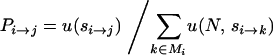
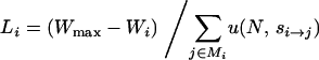
Starting with a population fixed for arbitrary genotype i, the probability of the appearance in any generation of a mutation destined to fix (unconditioned on identity) is 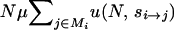, namely, the whole-genome mutation rate (NμL) times the average probability of fixation among all single-mutant neighbors of i (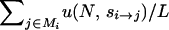). Here, N is the haploid population size, μ is the per-generation per-locus mutation rate, s_i→j is the selection coefficient acting on the mutation that carries the ith genotype to the jth genotype, and M_i is the set of all L single-mutant neighbors of genotype i. The fitness landscapes specifies fitness values W_i and W_j for genotypes i and j, respectively, and s_i→j is the normalized fitness difference (W_j − W_i)/W_i. Finally, u(N, s) is the fixation probability of a mutation with selection coefficient s and is given by 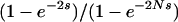, the haploid analog of Equation 10 of Kimura (1962), derived using the diffusion approximation. Since the expected waiting time for an event in units of a given time interval is the reciprocal of its rate per interval, starting with a population fixed for genotype i, the expected waiting time to the next mutation destined to fix is

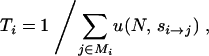(1)

now written in units of Nμ generations.

Starting from the lowest-fitness genotype, Equation 1 gives the expected time to the first fixation unconditioned on its identity. The probability that the fixation is to any given genotype j ∈ M_i is given by its normalized fixation probability

(2)

Expressions similar to Equations 1 and 2 have been presented previously by Gillespie (1984).

The expected time to the second fixation is also given by Equation 1. However, Equation 1 must now be evaluated conditioned on each possible first fixation, and the time to the second fixation unconditioned on identity is the average of these conditioned values weighted by the probabilities of each possible first fixation, given by Equation 2. In general the s_i→j's entering Equation 1 at each point in the process will be a function of the identity of all previous fixations and so the cumulative application of Equation 1 must be weighted by the probability of the fixation of each possible preceding succession of fixations. Because the number of mutations available to the currently fixed genotype is L at each step in the process, no simple closed-form solution appears to be available. However, a simplification is possible in the absence of sign epistasis. Because the probability of fixation for a beneficial mutation is much larger than that for a deleterious mutation, it seems reasonable to disregard the possibility of the latter event. In this case Equations 1 and 2 may be evaluated only over , the set of beneficial single-mutant neighbors of genotype i, and in the absence of sign epistasis the size of drops by one after each fixation. I used this simplification to arrive at a closed-form solution for the expected time from the lowest- to the highest-fitness genotype.

Individual-based computer simulations were performed to explore the consequences of the SSWM assumptions. In addition, the legitimacy of disregarding deleterious mutations was tested by comparing analytic results with those from stochastic computer simulations performed as follows. Beginning with the lowest-fitness genotype, Equation 1 was calculated over M_i, and the identity of the first fixation was drawn at random according to the probabilities given by Equation 2. This cycle was repeated until the highest-fitness genotype was fixed, evaluating Equations 1 and 2 over M_i (not ) at each step, and the mean elapsed time over 100 such evolutionary realizations was recorded.

Genetic constraint as a function of fitness landscape rank ordering:

To test the hypothesis that for landscapes lacking sign epistasis, landscape membership in rank ordering is associated with the time for a population to evolve from the lowest- to the highest-fitness genotype, I enumerated all possible rank orderings lacking sign epistasis for given L. For each rank ordering I generated a large number of random fitness landscapes as follows. I first drew 2^L − 2 fitness values uniformly distributed on the interval (W_min, W_max). Next I sorted these values together with W_min and W_max in ascending order. Finally I assigned each fitness value to the corresponding genotype as specified by the current rank ordering. For each fitness landscape I calculated the expected time for evolution by natural selection to carry a population from the lowest- to the highest-fitness genotype for some population size, using either the closed-form or stochastic methods described above.

Statistical tests:

The distribution of times among landscapes within rank orderings in which natural selection carries a population from the lowest- to the highest-fitness genotype is highly skewed to the left and distinctly nonnormal (not shown). Thus nonparametric tests of association were employed to assign statistical significance (Sokal and Rohlf 1981). To ensure that test statistics were correctly calculated, data were randomized with respect to rank ordering or population size. Test statistics calculated with these randomized data were not statistically significant.

Computer software:

All software was written in C and is available from the author upon request.

RESULTS

Time to evolve to the highest-fitness genotype:

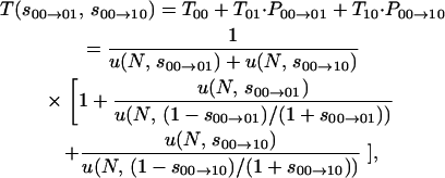
By disregarding reversions, which in the absence of sign epistasis are necessarily deleterious, a closed-form expression for the expected time to the all-1's genotype can easily be developed for arbitrary L, the number of interacting loci. Defining W_min ≡ 1 and W_max ≡ 2, for the case L = 2 we can write the expected time as

(3)

again in units of Nμ generations. Equation 3 illustrates that T(s_00→01, s_00→10) is the sum of three terms: the expected time to the first fixation unconditioned on identity (T₀₀, given by Equation 1) and the expected time to the alternative second fixations (T₀₁ and T₁₀, again given by Equation 1) weighted by the probabilities of each possible first fixation (P_00→01 and P_00→10, given by Equation 2).

In the absence of sign epistasis, 0 < s_00→01, s_00→10 < 1, and the graph of Equation 3 over this space is shown in Figure 1 for N = 1000. For most points in (s_00→01, s_00→10)-space, time to fixation of the “11” genotype is relatively low, although it rises quickly either if both s_00→01 and s_00→10 are < ∼0.1 or if either one is > ∼0.8. In the former case the contribution of T₀₀ to Equation 3 grows because the time for either first mutation to escape loss to drift is very large, although once fixed the time to fix the second mutation is short. In the latter case, since at least one first mutation has a relatively large selection coefficient, the first fixation will likely be of large effect and so occurs rather quickly. But the selection coefficient for the remaining mutation is (recall that W_max ≡ 2), which is necessarily now very small, and thus the time for the second mutation to escape loss to drift (T₀₁ or T₁₀) is large.

Figure 1.

Expected time for a population to evolve from the lowest- to the highest-fitness genotype on all possible fitness landscapes lacking sign epistasis for L = 2, given by Equation 3. s_00→10 and s_00→01 are the selection coefficients for the 10 and 01 genotypes, respectively, relative to the 00 genotype. Time is given in units of Nμ generations. N = 1000.

To verify the accuracy of this analytic SSWM treatment for L = 2, individual-based computer simulations were performed with N = 1000 for a range of values of s ≡ s_00→01 = s_00→10. These results are shown in Figure 2A for Nμ = 0.001, 0.01, and 0.1 as solid circles, crosses, and open circles, respectively, together with the analytic expectation given by Equation 3 (solid line). Very close correspondence is observed when Nμ is small, although deviations become more substantial as Nμ approaches 1.0 and the SSWM assumptions fail.

Figure 2.

Sensitivities of two-locus model as a function of s ≡ s_00→10 = s_00→01. Time is given in units of Nμ generations. (A) Equation 3 is shown as a solid line, and individual-based simulation results allowing back mutations are shown for Nμ = 0.001, 0.01, and 0.1 (solid circles, crosses, and open circles, respectively), with N = 1000. (B) Equation 3 for N = 10³ (solid line) and N = 10⁷ (dashed line); note that the y-axis is log transformed.

Figure 2B shows values of Equation 3 for N = 10³ (solid line) and 10⁷ (dashed line) for very small and very large values of s ≡ s_00→10 = s_00→01. The model is seen to exhibit sensitivity to population size only in these regions of parameter space. The sensitivity to small s is the consequence of the fact that for fixed s, the probability of fixation begins to increase as population size decreases below , when the population enters the neutral regime. This increase in fixation probability shortens T(s, s) for small s by reducing T₀₀ in Equation 3. By similar reasoning, T₀₁ and T₁₀ in Equation 3 are reduced as N declines for large s [and consequently small ]. This result is not an artifact of the diffusion approximation assumed in Equation 3: it is replicated in the analogous exact solution to the Moran model (J. Wakeley, personal communication).

By symmetry the minimum for Equation 3 must lie on the line s = s_00→01 = s_00→10, and substituting u(s) = 2s (Haldane 1927) for the diffusion solution of Kimura's yields a minimum when . Interestingly, epistasis exists for this value of s, since the fitness effect of the second 0 → 1 mutation is , which in this case is 0.5. Thus some epistasis is necessary to minimize this proxy for genetic constraint.

For L = 3 the expected time to the first fixation is given by Equation 1 and the remaining times are given by Equation 3, now weighted by the probability of each alternative first fixation given by Equation 2, again disregarding reversions. In this manner, algebraic expressions for the expected time to evolve from the lowest- to the highest-fitness genotypes for arbitrary L can be recursively constructed. However, as there are 2^L − 2 free parameters, no simple graphical representation of these results is possible for L > 2. Rather, these results are presented next as a function of fitness landscape rank orderings.

Constraint as a function of fitness landscape rank ordering:

In the absence of sign epistasis only one rank ordering for L = 2 exists, but eight rank orderings exist for L = 3, designated I–VIII and shown in Table 1. Recall that in general alleles may be relabeled so that the lowest-fitness (rank 8) genotype is “000” and also that in the absence of sign epistasis such relabeling means that the highest (rank 1) genotype is “111.” Furthermore, as previously noted, unless the second- and third-lowest-fitness genotypes (ranks 7 and 6) have exactly one 1 allele, the fitness ranking will exhibit sign epistasis. Without loss of generality, I assign these fitness ranks to the 001 and 010 genotypes, respectively. Thus the eight fitness rank orderings differ only in the ranks assigned to genotypes 100, 011, 101, and 110 and these are in italics in Table 1.

To see why there are eight rank orderings in Table 1, note first that to avoid sign epistasis, genotype 100 (the third genotype with exactly one 1 allele) cannot be more fit than either 110 or 101. Thus genotype 100 can assume only fitness rank 4 or 5. In the former case genotype 011 must occupy rank 5 and the remaining two genotypes may occur in either order, giving rise to rank orderings I and II in Table 1. Alternatively, if genotype 100 is assigned fitness rank 5, the three remaining genotypes may occur in any of the 3! = 6 possible orderings; these correspond to rank orderings III–VIII.

For each rank ordering in Table 1, I generated 1000 random fitness landscapes as described and for each landscape I calculated the expected time from the lowest- to the highest-fitness genotype in a population of size N = 1000 by the recursive application of Equations 1 and 2, disregarding the possibility of the fixation of (deleterious) reversion mutations. By the Kruskal-Wallis test, a highly significant effect of rank ordering on time exists (H = 97.997; d.f. = 7; P < 10⁻¹⁰). Results were indistinguishable when the possibility of reversion mutations was included using the stochastic approach described (not shown), as expected from the two-locus results in Figure 2A.

The coefficient of variance among times for landscapes within rank orderings is plotted against the mean time for landscapes within rank orderings in Figure 3 for N = 1000, graphically illustrating these results. Some insight into the rank-ordering characteristics responsible for the variation in mean and variance in time to evolve from the lowest- to the highest-fitness genotypes is possible. For example, why are fitness ranks III and VI fastest?

Figure 3.

Coefficient of variance plotted against mean time to evolve from lowest- to highest-fitness genotype for each fitness landscape rank ordering in Table 1. Values from 1000 random landscapes sampled for each rank ordering are shown. Time is given in units of Nμ generations. N = 1000.

Evolving populations will most often fix the beneficial mutation of largest effect at each step (Equation 1), and for each rank ordering in Table 1 the most likely first fixation will therefore be to genotype 100, since its rank (4 or 5) ensures that on all landscapes its fitness will be higher than that of either of the other single-mutant neighbors of 000 (with ranks 6 and 7). Conditioned on this first fixation, on landscapes belonging to rank orderings III and VI the most likely second fixation will be to the genotype of rank 3, whereas on the other six rank orderings, the most likely genotype fixed next will have rank 2. The evolutionary speed observed for ranks III and VI is the consequence of the fact that the fitness of the penultimate genotype fixed along the most likely evolutionary trajectory on these fitness landscapes is lower, thereby leaving additional selective effect to drive the final fixation. This is similar to the dynamics observed in the two-locus treatment (Figure 1), in which T(s_00→01,s_00→10) is large when either s_00→01 or s_00→10 is large.

We can similarly understand the difference in variance observed between rank orderings III and VI. Here the effect is due to the ranks of the alternate genotypes fixed after the second most likely first fixation. In all eight rank orderings the second most likely first fixation yields the 010 genotype, and conditioned on this first fixation, natural selection will proceed via the fixation of either the 011 or 110 genotype. The difference in variance between rank orderings III and VI seen in Figure 3 is due to the difference in variance in ranks of these two genotypes: lower in the former (ranks 2 and 3) than in the latter (ranks 2 and 4).

To further test the strength of association between fitness landscape rank ordering and time to evolve from the lowest- to the highest-fitness genotype, I repeated the simulations for a range of population sizes spanning eight orders of magnitude using a common set of 1000 fitness landscapes for each rank ordering in Table 1. In each case, a highly significant statistical effect of rank ordering on time was again observed by the Kruskal-Wallis test (minimum observed test statistic across eight cases: H = 97.997; d.f. = 7; P < 10⁻¹⁰). The mean time increases with population size for all rank orderings, as expected (Figure 2B), and as population size increased the mean time converges to a rank-ordering-specific value. This is a consequence of the fact that the population-size dependence seen in Figure 2B covers an ever-smaller spectrum of selection coefficients as population size grows (not shown); the probability that mutationally adjacent genotypes should have sufficiently small fitness differences to exhibit population size-dependent behavior thus vanishes. Mean times for each rank ordering calculated for population sizes from 10 to 10⁵ are presented in Figure 4; values for larger populations were indistinguishable from those for 10⁵. It is clear from Figure 4 that a strong correlation exists between rank ordering and mean time rank order, and by Friedman's method for randomized blocks this association is highly significant (X² = 44.67, d.f. = 7, P = 1.6 × 10⁻⁷). In other words, the identity of the fastest (second-fastest, etc.) fitness landscape rank ordering is largely independent of population size. Interestingly the population size at which the mean time converges also shows sensitivity to rank ordering identity.

Figure 4.

Mean time to evolve from lowest- to highest-fitness genotype for each fitness landscape rank ordering in Table 1, for five different effective population sizes (cross, N = 10; open circle, N = 100; solid circle, N = 10³; open square, N = 10⁴; solid square, N = 10⁵). Values are from 1000 random landscapes for each rank ordering. Time is given in units of Nμ generations.

For L = 4, there are 70,016 fitness landscape rank orderings that lack sign epistasis (available from the author on request). For each rank ordering, I generated 100 random fitness landscapes as before and calculated the time for natural selection to carry a population from the lowest- to the highest-fitness genotype for N = 1000. By the Kruskal-Wallis test, a highly significant effect of rank ordering on time again exists (H = 189,832.358; d.f. = 70,015; P < 10⁻¹⁰). Exhaustive exploration for L > 4 was not attempted as the number of rank orderings appears prohibitively large, although the general principles observed for L < 5 are expected to apply to landscapes with arbitrary L.

DISCUSSION

Functional interactions between loci can have the consequence that the fitness effect of a mutation at one locus may be conditional on the allelic state at one or more other loci. Such effects are called epistatic and can have profound evolutionary implications because they raise the possibility that natural selection will regard the same mutation differently when it occurs in different genetic backgrounds. Wright (1932) defined the fitness landscape to permit the graphical representation of mutational fitness effects in the presence of epistasis and noted that as a consequence of epistasis landscapes could possess multiple fitness peaks that would sharply constrain natural selection. More recently, attention has focused on the effects of conditional selective neutrality (e.g., van Nimwegen and Crutchfield 2000) and on the development of a general algebraic theory of fitness landscapes (Stadler 2003).

If genotypic fitness values are continuous then the number of possible fitness landscapes is uncountable, making an exhaustive survey of this space impossible. In contrast, the number of fitness landscape rank orderings is finite. Furthermore it follows by symmetry that if genotypic fitness values are independent and identically distributed (i.i.d.), then rank orderings partition the space of all possible fitness landscapes into equal-sized pieces. This is because a set of deviates drawn from a fixed distribution is equally likely to define any given rank ordering. Since fitness landscape membership in rank ordering is a good proxy for genetic constraint on evolution by natural selection, under the assumption that genotypic fitness values are i.i.d., it follows that surveying all rank orderings represents a good proxy for surveying all fitness landscapes. Thus for large L for which exhaustive sampling appears prohibitive, sampling rank orderings will provide a more thorough survey of the space of possible fitness landscapes than randomly sampling fitness landscapes directly.

Two theoretical shortcomings should be noted. The SSWM approximation employed disregards the transit time through frequency space for a mutation destined to fix. Perhaps most importantly, this means that I have ignored genetic recombination, which nevertheless may have profound evolutionary implications as it can disrupt allelic combinations before they reach fixation (or equally, increase the rate of production of high-fitness allelic combinations). In the limit free recombination renders epistasis irrelevant since cooccurring alleles are not reliably cotransmitted to offspring, and the sensitivity of the level of genetic constraint predicted for each rank ordering in the presence of modest recombination remains an open question. Results here are, however, applicable to fitness interactions among mutations at the scale of protein- or RNA-encoding genes, which recombination is less likely to disrupt during transit. Additionally I have implicitly assumed that fitness interactions between loci remain invariant during the course of population evolution from the lowest- to the highest-fitness genotype. Certainly an organism's environment may change during this time interval, which may affect epistatic effects. However, in the absence of empirical knowledge of how environmental shifts affect interactions among genotypic fitness values, the results presented here may be interpreted as giving insight into the constraint on evolution acting on populations between such environmental shifts (Gillespie 1984).

The greatest limitation presently in application of the rank-ordering approach to characterizing genetic constraint is empirical: only limited measurements of actual genotypic fitness landscapes exist. We as yet know little about the frequency or size of epistatic effects between mutations for any phenotype in any organism (Weinreich et al. 2005). One example of the sort of data required comes from work in the TEM alleles of the β-lactamase antibiotic gene by Hall (2002). Here a subset of all possible mutational intermediates between low- and high-activity genetic variants differing at a small number of nucleotides was constructed by site-directed mutagenesis and the resulting antibiotic resistance phenotype was characterized. Epistasis at every locus was detected, including two cases of sign epistasis. However, even taking antibiotic resistance as a proxy for fitness, because Hall constructed only a subset of allelic combinations we are as yet unable to apply the rank-ordering formalism even to this system. Nevertheless, no technical obstacles to collecting these missing data exist.

Once data of this sort become available from several experimental systems, it will be possible to address important questions raised by the rank-ordering formalism developed here. First, it is clear that the assumption that genotypic fitness values are independently distributed is unrealistic, implying that some rank orderings will be much more common in nature than others. But the form and intensity of fitness correlations is generally unknown, as are its consequences for genetic constraint. In other words, are naturally occurring fitness rank orderings anomalously “fast” or “slow” compared to expectation under the i.i.d. assumption? In this report I have explored a nonrandom set of rank orderings, namely those lacking sign epistasis, and this imposes some correlation on fitness values of mutationally adjacent genotypes. However, sign epistasis is common in nature (Weinreich et al. 2005) so the exclusion of the remaining rank orderings does not adequately address this problem. Furthermore, substantial variation in constraint exists among fitness landscapes within rank orderings (Figure 3). It will thus be interesting and important to determine similarly whether naturally occurring fitness landscapes are anomalously fast or slow given the rank ordering they represent. Finally, we are even perhaps without intuition about the effects of changing environment on epistatic interactions; again, empirical data will greatly enhance our ability to interpret results developed for the rank-ordering formalism, which could then be extended to incorporate the effects of temporally changing fitness landscapes.

This line of thinking sheds further light on the practical meaning of L, the number of loci in the model. Systems such as Hall's (2002) begin with an assumption that mutations at only some loci are relevant for the problem at hand. Nevertheless, application of the rank-order formalism to all allelic combinations of this subset of loci will yield accurate inferences regarding the genetic constraint imposed on evolution by natural selection at those loci. Put another way, if knowledge of a particular biological system motivates an a priori assumption that some loci may be disregarded, the rank-ordering apparatus may legitimately be applied to the remaining loci.

Throughout, the mean time to evolve from the lowest- to the highest-fitness genotype has been employed as a proxy for genetic constraint. However, we have noted that this quantity can increase as the fitness of the penultimate genotype approaches W_max (e.g., Figure 1), in spite of the fact that populations fixed for this genotype will by definition already be very fit. This suggests the possibility that even though an evolving population may quickly reach fitness very near W_max on some fitness landscapes, my choice of metric penalizes such landscapes, and thus the strong association between rank ordering and mean time to fix the fittest genotype observed may be artifactual. To address this concern I explored another proxy for genetic constraint.

Writing W(t) as the fitness of the genotype fixed at time t, define the “adaptive lag” of a fitness landscape as the time integral of W_max − W(t) evaluated over the time course of the entire process. Unlike the mean time to evolve to the highest-fitness genotype, the adaptive lag down-weights the time spent late in the process as W_max − W(t) declines. The expected adaptive lag contributed by genotype i is W_max − W_i multiplied by the expected time spent by a population fixed for this genotype or algebraically,

(4)

Employing this expression in place of Equation 1, the adaptive lag (in units of Nμ generations) may be computed for any fitness landscape lacking sign epistasis following the recursive approach outlined above. To test the sensitivity of the L = 3 results to choice of metric, I again generated 1000 random fitness landscapes for each rank ordering defined in Table 1 and computed the adaptive lag for each setting N = 1000. By the Kruskal-Wallis test, a highly significant effect of rank ordering on the mean adaptive lag across landscapes was again observed (H = 200.979; d.f. = 7; P < 10⁻¹⁰). Not surprisingly, the two metrics have a negative correlation (r² = 0.35): faster rank orderings are “fueled” by a larger adaptive lag. However, slower rank orderings appear not to be artifactually penalized by my original choice of metric.

The rank-ordering formalism developed here bears some similarity to recent work of Orr (2002, 2003, 2005), employing extreme value theory. Obviously the expected value of an arbitrary selection coefficient (e.g., s_i→j) depends on the (unknown) distribution from which fitness values are drawn. However, Orr has shown that for a very broad class of distributions the expected ratio of two selection coefficients (e.g., s_i→j/s_k→l) depends only on the fitness ranks of genotypes i, j, k, and l and not on the distribution itself. Because expressions such as Equation 2 (the probability of fixing genotype j from genotype i) can be closely approximated by a ratio of selection coefficients [recalling that (Haldane 1927)], Orr (2002, 2003, 2005) has succeeded in developing distribution-independent expectations for a great many sophisticated quantities that are functions of fixation probabilities.

In contrast, the application of extreme value theory to the expected time to fixation is less satisfactory, fundamentally because Equation 1 and its analogs cannot be written as a ratio of selection coefficients. Rather, expressions for expected time to fixation take the form of the reciprocal of selection coefficients, and so results under extreme value theory do not share the elegant near distribution independence enjoyed by those developed by Orr.

Low genetic constraint as defined here is closely related to the notion of evolvability, the ability of an organism to produce heritable, adaptive variants among its progeny (Wagner and Altenberg 1996; Kirschner and Gerhart 1998), and high evolvability suggests that population fitness increases rapidly. However, should empirical data of the sort described above be developed and be found to demonstrate anomalously low levels of genetic constraint (relative to expectations based on i.i.d. fitness values), it will be important to note that this does not necessarily imply the action of selection for evolvability. One obvious point to be borne in mind is that the null expectation is biologically unrealistic: fitness values for mutationally adjacent genotypes are likely to be correlated. More generally, determining the mean time in which natural selection carries a population across a given fitness landscape answers questions about the evolvability of the landscape but is agnostic on the question of the origin of such evolvability. Nothing will have been learned about either temporal changes in the genetic constraint acting on a landscape or the mechanistic underpinnings of such constraint, both of which are fundamental to claims of selection for evolvability.

I originally tested the ability of the fitness landscape rank-ordering apparatus to predict the time for natural selection to carry a population from the lowest- to the highest-fitness genotype using the class of fitness landscapes lacking sign epistasis as a negative control. I imagined that no heterogeneity in genetic constraint existed among such landscapes. To the contrary, I found that landscape membership in rank ordering provides both predictive and explanatory power to understand variation in the mean time for natural selection to carry populations from the lowest- to the highest-fitness genotypes. The association between rank-ordering membership and this proxy for genetic constraint was observed at a range of population sizes, and furthermore the relative level of constraint exhibited by each rank ordering was also almost invariant across N (Figure 4).

That the identity of the fastest (second fastest, etc.) rank ordering is largely independent of population size in the absence of sign epistasis is perhaps not surprising. In this case all mutations that differentiate an arbitrary genotype from the highest-fitness genotype are necessarily beneficial, and I found that the evolutionary trajectory followed through genotypic sequence space is primarily constructed of such mutations. This was evidenced by the fact that results were indistinguishable when Equations 1 and 2 were evaluated over M_i and , which differ only in the inclusion of deleterious reversion mutations. Therefore we might expect that the relative level of genetic constraint exhibited by each rank ordering is fairly insensitive to population size (after normalizing by Nμ), since the probability of (and thus the expected waiting time until) fixation of beneficial mutations is almost independent of this quantity (Haldane 1927).

In contrast, evolutionary dynamics in the presence of sign epistasis are not necessarily independent of population size. This is the consequence of the fact that on such fitness landscapes some of the mutations that differentiate a focal genotype from the highest-fitness genotype may be deleterious in the focal genotype, raising the possibility of multiple peaks on the landscape, i.e., genotypes in which all mutations are individually deleterious (Wright 1932). Thus the evolutionary trajectory followed by a population on a fitness landscape with sign epistasis may require “escape” from local, suboptimal peaks, the dynamics of which are sensitive to population size in a nonmonotonic manner (Carter and Wagner 2002; Iwasa et al. 2004; Weinreich and Chao 2005). The implication of this nonmonotonicity due to sign epistasis for the predictive and explanatory utility of the fitness landscape rank-ordering apparatus, and in particular on the near invariance of the relative level of genetic constraint exhibited by rank orderings across a range of population sizes, is unclear. Additionally, while sign epistasis is necessary for multiple peaks on the fitness landscape, it is not sufficient (Burch and Chao 1999; Weinreich et al. 2005), suggesting further that evolutionary constraints other than escape from local fitness peaks may be important on landscapes with sign epistasis. No general treatment of genetic constraint in the presence of sign epistasis yet exists.

References

- Burch, C. L., and L. Chao, 1999. Evolution by small steps and rugged landscapes in the RNA virus ø6. Genetics 151: 921–927. [DOI] [PMC free article] [PubMed] [Google Scholar]
- Bustamante, C. D., R. Nielsen, S. A. Sawyer, K. M. Olsen, M. D. Purugganan et al., 2002. The cost of inbreeding in Arabidopsis. Nature 416: 531–534. [DOI] [PubMed] [Google Scholar]
- Carter, A. J. R., and G. P. Wagner, 2002. Evolution of functionally conserved enhancers can be accelerated in large populations: a population-genetic model. Proc. R. Soc. Lond. Ser. B 269: 953–960. [DOI] [PMC free article] [PubMed] [Google Scholar]
- Dickerson, R. E., 1971. The structure of cytochrome c and the rates of molecular evolution. J. Mol. Evol. 1: 26–45. [DOI] [PubMed] [Google Scholar]
- Fay, J. C., G. J. Wyckoff and C.-I Wu, 2002. Testing the neutral theory of molecular evolution with genomic data from Drosophila. Nature 415: 1024–1026. [DOI] [PubMed] [Google Scholar]
- Fisher, R. A., 1918. The correlation between relatives on the supposition of Mendelian inheritence. Trans. R. Soc. Edinb. 52: 399–433. [Google Scholar]
- Gillespie, J. H., 1984. Molecular evolution over the mutational landscape. Evolution 38: 1116–1129. [DOI] [PubMed] [Google Scholar]
- Gillespie, J. H., 1991. The Causes of Molecular Evolution. Oxford University Press, Oxford.
- Haldane, J. B. S., 1927. A mathematical theory of natural and artificial selection. Part V. Proc. Camb. Philos. Soc. 23: 838–844. [Google Scholar]
- Haldane, J. B. S., 1957. The cost of natural selection. J. Genet. 55: 511–524. [Google Scholar]
- Hall, B. G., 2002. Predicting evolution by in vitro evolution requires determining evolutionary pathways. Antimicrob. Agents Chemother. 46: 3035–3038. [DOI] [PMC free article] [PubMed] [Google Scholar]
- Hey, J., and R. M. Kliman, 2002. Interactions between natural selection, recombination and gene density in the genes of Drosophila. Genetics 160: 595–608. [DOI] [PMC free article] [PubMed] [Google Scholar]
- Horn, J., D. E. Goldberg and K. Deb, 1994. Long path problems. Lect. Notes Comput. Sci. 866: 149–158. [Google Scholar]
- Iwasa, Y., F. Michor and M. A. Nowak, 2004. Stochastic tunnels in evolutionary dynamics. Genetics 166: 1571–1579. [DOI] [PMC free article] [PubMed] [Google Scholar]
- Jensen-Seaman, M. I., T. S. Furey, B. A. Payseur, Y. Lu, K. M. Roskin et al., 2004. Comparative recombination rates in the rat, mouse and human genomes. Genome Res. 14: 528–538. [DOI] [PMC free article] [PubMed] [Google Scholar]
- Kauffman, S. A., 1993. The Origins of Order. Oxford University Press, New York/Oxford.
- Kimura, M., 1962. On the probability of fixation of mutant genes in a population. Genetics 47: 713–719. [DOI] [PMC free article] [PubMed] [Google Scholar]
- Kimura, M., 1968. Evolutionary rate at the molecular level. Nature 217: 625–626. [DOI] [PubMed] [Google Scholar]
- Kimura, M., 1969. The rate of molecular evolution considered from the standpoint of population genetics. Proc. Natl. Acad. Sci. USA 63: 1181–1188. [DOI] [PMC free article] [PubMed] [Google Scholar]
- Kimura, M., 1983. The Neutral Theory of Molecular Evolution. Cambridge University Press, Cambridge, UK.
- Kirschner, M., and J. Gerhart, 1998. Evolvability. Proc. Natl. Acad. Sci. USA 95: 8420–8427. [DOI] [PMC free article] [PubMed] [Google Scholar]
- Kreitman, M., and H. Akashi, 1995. Molecular evidence for natural selection. Annu. Rev. Ecol. Syst. 26: 403–422. [Google Scholar]
- Maynard Smith, J., 1970. Natural selection and the concept of a protein space. Nature 225: 563–565. [DOI] [PubMed] [Google Scholar]
- Moran, P. A. P., 1970. Haldane's dilemma and rate of evolution. Ann. Hum. Genet. 33: 245. [DOI] [PubMed] [Google Scholar]
- Muse, S. V., and B. S. Gaut, 1997. Comparing patterns of nucleotide substitution rates among chloroplast loci using the relative ratio test. Genetics 146: 393–399. [DOI] [PMC free article] [PubMed] [Google Scholar]
- Orr, A. H., 2002. The population genetics of adaptation: the adaptation of DNA sequences. Evolution 56: 1317–1330. [DOI] [PubMed] [Google Scholar]
- Orr, A. H., 2003. The distribution of fitness effects among beneficial mutations. Genetics 163: 1519–1526. [DOI] [PMC free article] [PubMed] [Google Scholar]
- Orr, A. H., 2005. The probability of parallel evolution. Evolution 59: 216–220. [PubMed] [Google Scholar]
- Provine, W. B., 1986. Sewall Wright and Evolutionary Biology. University of Chicago Press, Chicago.
- Ridley, M., 1993. Evolution. Blackwell Scientific Publications, Boston.
- Sawyer, S., R. J. Kulathinal, C. D. Bustamante and D. L. Hartl, 2003. Bayesian analysis suggests that most amino acid replacements in Drosophila are driven by positive selection. J. Mol. Evol. 57: S154–S164. [DOI] [PubMed] [Google Scholar]
- Smith, N. G. C., and A. Eyre-Walker, 2002. Adaptive protein evolution in Drosophila. Nature 415: 1022–1024. [DOI] [PubMed] [Google Scholar]
- Sokal, R. R., and F. J. Rohlf, 1981. Biometry. W. H. Freeman, New York.
- Stadler, P. F., 2003. Spectral landscape theory, pp. 221–272 in Evolutionary Dynamics: Exploring the Interplay of Selection, Accident, Neutrality, and Function, edited by J. P. Crutchfield and P. Schuster. Oxford University Press, Oxford.
- van Nimwegen, E., and J. P. Crutchfield, 2000. Metastable evolutionary dynamics: crossing fitness barriers or escaping via neutral paths? Bull. Math. Biol. 62: 799–848. [DOI] [PubMed] [Google Scholar]
- Wagner, G. P., and L. Altenberg, 1996. Perspective: complex adaptations and the evolution of evolvability. Evolution 50: 967–976. [DOI] [PubMed] [Google Scholar]
- Wallace, B., 1991. Fifty Years of Genetic Load: An Odyssey. Cornell University Press, Ithaca, NY.
- Weinreich, D. M., 2001. The rates of molecular evolution in rodent and primate mitochondrial DNA. J. Mol. Evol. 52: 40–50. [DOI] [PubMed] [Google Scholar]
- Weinreich, D. M., and L. Chao, 2005. Rapid evolutionary escape by large populations from local fitness peaks is likely in nature. Evolution 59: 1175–1182. [PubMed] [Google Scholar]
- Weinreich, D. M., and D. M. Rand, 2000. Contrasting patterns of non-neutral evolution in proteins encoded in nuclear and mitochondrial genomes. Genetics 156: 385–399. [DOI] [PMC free article] [PubMed] [Google Scholar]
- Weinreich, D. M., R. A. Watson and L. Chao, 2005. Sign epistasis and genetic constraint on evolutionary trajectories. Evolution 59: 1165–1174. [PubMed] [Google Scholar]
- Wright, S., 1930. Review of the genetical theory of natural selection. J. Hered. 21: 349–356. [Google Scholar]
- Wright, S., 1932. The roles of mutation, inbreeding, crossbreeding and selection in evolution, pp. 356–366 in Proceedings of the Sixth International Congress of Genetics, edited by D. F. Jones. Brooklyn Botanic Garden, Menasha, WI.
- Yang, Z., and R. Nielsen, 1998. Synonymous and nonsynonymous rate variation in nuclear genes of mammals. J. Mol. Evol. 46: 409–418. [DOI] [PubMed] [Google Scholar]
- Zeng, L.-W., J. M. Comeron, B. Chen and M. Kreitman, 1998. The molecular clock revisited: the rate of synonymous vs. replacement change in Drosophila. Genetica 102/103: 369–382. [PubMed] [Google Scholar]
- Zuckerkandl, E., and L. Pauling, 1965. Evolutionary divergence and convergence in proteins, pp. 97–166 in Evolving Genes and Proteins: A Symposium, edited by V. Bryson and H. Vogel. Academic Press, New York.