The Timing of Entry Into Fatherhood in Young, At-Risk Men

Abstract

Timing of first fatherhood was examined in a sample of 206 at-risk, predominantly White men, followed prospectively for 17 years. An event history analysis was used to test a model wherein antisocial behavior, the contextual and familial factors that may contribute to the development of antisocial behavior, and common correlates of such behavior, including academic failure, substance use, and early initiation of sexual behaviors, lead both directly and indirectly to an early transition to fatherhood. Having a mother who was younger at first birth, low family SES, poor academic skills, failure to use condoms, and being in a cohabitating or marital relationship predicted entry into fatherhood. Implications of the findings for prevention of and intervention with early fathering are discussed.

The Timing of Entry Into Fatherhood in Young, At-Risk Men

A greater understanding of factors associated with positive parenting for fathers would aid in designing prevention programs to help break the intergenerational transmission of risk for problem outcomes such as antisocial behavior and substance use (Capaldi, Pears, Patterson, & Owen, 2003). An important aspect of such knowledge is examination of developmental factors related to the age of entry into biological fatherhood. Adolescent fathers are costly to society; they are less likely than older fathers to live with the mother and child and to be able to provide adequate financial support (Jaffee, Caspi, Moffitt, Taylor, & Dickson, 2001; Lerman, 1993). Further, there is evidence that adolescent parents--both mothers and fathers--provide a poorer environment and less skilled parenting for their child than older parents (Becker, 1987; Berlin, Brady-Smith, & Brooks-Gunn, 2002; Black et al., 2002).

The difficulties adolescent parents face may be due in part to factors associated with the timing of their transition to parenthood. Societal norms govern the age at which the transitions into various roles (e.g., full-time worker, marital partner, or parent) should be made (Hogan & Astone, 1986; Neugarten, Moore, & Lowe, 1965). Thus, role transitions may be age appropriate or off time--either too early or too late (Hogan & Astone, 1986). Off-time transitions may have serious consequences for both role performance and the timing of subsequent transitions (Hogan & Astone). For example, adolescent parents have difficulties in the parenting role and may speed the transition out of school by dropping out (Berlin et al., 2002; Upchurch & McCarthy, 1990). Not all off-time transitions are detrimental to role performance, however. For example, fathers who delay parenthood until their mid- to late-30s and beyond show greater involvement with and more nurturant behavior toward their children than on-time fathers (e.g., Cooney, Pedersen, Indelicato, & Palkovitz, 1993; Heath, 1994).

The processes related to the timing of entry into first fatherhood are not well known. Extant studies have tended to involve correlates of adolescent fatherhood (e.g., Thornberry, Smith, & Howard, 1997). A notable exception is Jaffee et al.’s (2001) examination of factors associated with the timing of fatherhood through age 26 years in a sample of New Zealand men. Being born to a teen mother, living with a single parent, early initiation of sexual activity, history of conduct disorder, and leaving school before age 16 years increased the likelihood of becoming a father between the ages of 14 and 26 years.

Early-timed transitions may be particularly detrimental to role performance because they are made prior to developmental readiness. Positive development is hierarchical and integrative, whereby the developments at one life stage rest on the developmental accomplishments and skills acquired in prior stages (Cicchetti & Rogosch, 2002). Early role transitions may leave the key tasks of critical developmental periods uncompleted. Conversely, early role transitions may result from an inability to master key developmental tasks and from a perceived lack of alternatives. For instance, adolescents who are unable to succeed at school may feel that they have fewer chances for continuing their education and may not take adequate precautions against early parenthood. Thus, risk factors associated with failure to make key developmental accomplishments also increase the likelihood that transitions will be off time.

We posit that antisocial behavior is such a risk factor because it is associated with difficulties completing key social and academic developmental tasks of childhood and adolescence (Capaldi, 1992), and that these developmental failures are associated with early transitions into some adult roles (Burton, Obeidallah, & Allison, 1996; Capaldi & Shortt, 2003). Compared to their peers, youths at risk for the development of conduct problems in childhood because of problematic family factors (e.g., poor parenting) are more likely to develop antisocial behavior and to experience failures at the normative tasks of adolescence and young adulthood, including completing school (Elliott & Voss, 1974) and becoming consistently employed. Thus, youths at risk for antisocial behavior are also at particular risk for off-time transitions such as early entry into parenthood.

The Oregon Youth Study: Neighborhood Crime Effects on Risk for Antisocial Behavior

The current study extended further into the life course than studies of adolescent fathering by using an event history approach to examine the onset of fatherhood for young at-risk men from ages 13 – 14 years through ages 25 – 26 years. This study expands upon the Jaffee et al. (2001) study mentioned above by (a) using a U.S. sample in which 50% of the participants experienced fatherhood by ages 25 – 26 years (vs. 19% by age 26 years in the Jaffee et al. sample); (b) examining the contribution of proximal factors, including relationship status and sexual risk behaviors in addition to familial risk and problem behaviors; (c) using yearly measurement of individual and proximal risk factors; and (d) featuring a largely working-class sample at risk for antisocial behaviors.

The Oregon Youth Study is a sample of primarily White men, followed yearly from the ages of 9 – 10 to 25 – 26 years, who were at risk for early deviance because they were raised in neighborhoods with higher rates of juvenile delinquency than surrounding neighborhoods in a medium-sized metropolitan area. The amount of crime in a neighborhood is a significant risk factor for antisocial and externalizing behavior (e.g., Seidman et al., 1998; Simcha-Fagan & Schwartz, 1986; Stouthamer-Loeber, Loeber, Wei, Farrington, & Wikstrom, 2002). For example, Hill, Howell, Hawkins, and Battin-Pearson (1999) found that children in neighborhoods in which many youths were in trouble were three times more likely to join a gang in adolescence than their peers in less problematic neighborhoods. Youths in high-crime neighborhoods may believe that antisocial behavior is acceptable. Additionally, they have greater exposure to such behavior and more chances of associating with delinquent peers (Ingoldsby & Shaw, 2002; Sampson, 1997). A number of other neighborhood contextual factors also have been implicated in the development of antisocial behavior (Ingoldsby & Shaw), but neighborhood crime was the selection factor for this particular sample. Thus, the youths in the Oregon Youth Study lived in a context that put them at risk for antisocial and delinquent behaviors, which in the model presented below is posited to be a major factor affecting the timing of fatherhood in these men.

Factors Affecting Timing of Fatherhood in At-Risk Men

Summarized in Figure 1 are the three domains of developmental factors, namely familial, individual, and proximal, posited to be associated with early timing of fatherhood in at-risk young men. The model is based on research on the correlates of early fatherhood in both at-risk and nonrisk samples. Lower socioeconomic status (SES), being the child of a mother who was young at the birth of her first child, and multiple parental transitions form a constellation of family contextual risk factors that are both general risk factors for antisocial behavior via unskilled parenting (Capaldi & Patterson, 1994) and specific risk factors for early onset of intercourse in adolescence (Capaldi & Patterson, 1994; Hardy, Astone, Brooks-Gunn, Shapiro, & Miller, 1998). Age of the mother at first birth of her child has been investigated in at-risk samples (e.g., Hardy et al., 1998) but has also been shown to be a risk factor for youths in normative samples. Low SES in the family of origin has also been linked directly to early entry into fatherhood, even when antisocial behavior is accounted for (Fagot, Pears, Capaldi, Crosby, & Leve, 1998; Xie, Cairns, & Cairns, 2001) in both at-risk (e.g., Thornberry et al., 1997) and nonrisk samples (e.g., Hanson, Morrison, & Ginsburg, 1989). Low SES involves fewer years of education and lower occupation levels, and thus may indicate off-time transitions in the life courses of the parents.

Figure 1.

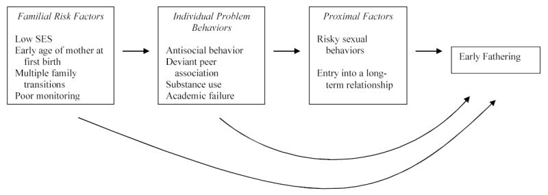
Conceptual model for early entry into fatherhood.

A further familial risk factor is parents’ failure to adequately monitor children’s whereabouts and activities, a key aspect of unskilled parenting that has been linked to delinquency and early initiation of drug use and sexual behaviors (Chilcoat, Dishion, & Anthony, 1995; Metzler, Noell, Biglan, Ary, & Smolkowski, 1994; Miller, Forehand, & Kotchick, 1999; Patterson & Stouthamer-Loeber, 1984). Higher numbers of parental transitions also directly predict earlier age at onset of intercourse, controlling for parental supervision and other risk factors (Capaldi, Crosby, & Stoolmiller, 1996). Through witnessing the parents’ relationships with several partners, the adolescent may come to feel that monogamy is not important and early sexual involvement is acceptable.

These familial risk factors place youths at higher risk for individual problem behaviors, including antisocial behavior and association with delinquent peers, academic failure, and substance use. A number of studies of at-risk and nonrisk samples have documented that young men who father children during their adolescence have higher rates of aggression (e.g., Scaramella, Conger, Simons, & Whitbeck, 1998) and delinquency (e.g., Fagot et al., 1998) compared to their nonfather peers. Additionally, boys’ risk for becoming fathers during their teens is increased through affiliations with aggressive peers who have problems in school (Xie et al. 2001). Direct links between substance use and early fatherhood also have been found, as well as links between substance use and early initiation of sexual intercourse (e.g., Kessler et al., 1997; Thornberry et al., 1997). Antisocial behavior, substance use, and early age at first intercourse may be interrelated because adolescents who engage in antisocial behavior are likely to have poorer impulse control and a greater predilection for engaging in risk-taking behaviors (Gottfredson & Hirschi, 1990; Newcomb & McGee, 1991).

Finally, in this constellation of individual problem behaviors, poor academic achievement and school dropout are consistently related to early fathering across at-risk and nonrisk samples (e.g., Fagot et al., 1998; Gest, Mahoney, & Cairns, 1999). Low achieving youths may feel they have fewer prospects of higher education and high paying jobs; thus, they have less incentive to protect against unplanned pregnancies (Hanson et al., 1989). We posit that academic failure and associated high school dropout are important factors in early entry into fathering as failure in one key developmental domain increases the risk of early role transition.

Next in the developmental sequence are the proximal factors of risky sexual behaviors and entry into longer-term relationships. The risky sexual behaviors all relate to levels of exposure for conception, as the more frequently unprotected intercourse occurs, the more likely is conception. Sexual intercourse puts adolescents at risk for early entry into fatherhood (Jaffee et al., 2001; Stouthamer-Loeber & Wei, 1998; Thornberry et al., 1997). Frequency of sexual intercourse and number of sexual partners are related to the numbers of pregnancies caused by adolescent boys, and condom use is negatively related to number of pregnancies (Goodyear, Newcomb, & Allison, 2000). Adolescent boys who are dating regularly have more opportunities to make the transition to parenthood (Marini, 1984) and are more likely than their peers to father children before age 20 years (Hanson et al., 1989). In a prior study with the Oregon Youth Study sample, antisocial behavior and substance use at age 20 years predicted higher rates of lifetime sexual risk behaviors, including higher frequency of intercourse, higher numbers of sexual partners, and lower rates of condom use (Capaldi, Stoolmiller, Clark, & Owen, 2002).

Timing of Fatherhood Across Early Adulthood

Little is known about the predictors of the timing of first fatherhood into adulthood (Forste, 2002), and it is unclear whether factors that predict adolescent fatherhood would continue to show the same degree of association into adulthood in an at-risk sample. Most of the familial risk factors, namely SES, mother’s age at her first birth, and number of parental transitions, are expected to predict timing of fatherhood in adulthood. They are posited to be associated with expectations regarding what is normative or appropriate timing for role transitions into marriage and parenthood. Indeed, age of mother at first birth appears to have effects on timing of parenthood across adolescence and adulthood for both women and men (Hardy et al., 1998), and parents who have experienced a higher number of partner changes or transitions tended to initiate parenthood at earlier ages (Capaldi & Patterson, 1991). Families with higher SES levels, particularly professional families and their offspring, may choose careers involving prolonged higher education and are likely to put off the transition to parenthood. Therefore, SES may be expected to show a linear association with timing of fatherhood. Of the contextual factors, only parental supervision is posited to show an association to age at first fatherhood that varies across time; as the youth grows older and leaves the parental home, supervision during childhood and adolescence should no longer affect the timing of fatherhood.

It might be assumed that individual problem behaviors would be predictive only of early fatherhood and would not discriminate the timing of fatherhood past adolescence, as the men mature and reach the ages at which it is normative to make the transition to parenthood. Problem behaviors, however, appear to be part of a pattern of disinhibition and risk taking that show a relatively normal distribution and that may be associated with sexual activity and failure to use contraception, which are as likely to lead to pregnancy in adulthood as in adolescence. Thus, the effects of individual problem behaviors on the risk for fathering might still be significant in the 20s. Jaffe and colleagues (2001) found that a history of conduct disorder and leaving school before age 16 years had constant effects on the risk of fathering across adolescence and young adulthood. Finally, the effects of sexual and relationship behaviors should be constant across time because both sets of behaviors carry the same risk for fathering a child at any age.

Overview of the Study

The current study had two goals: (a) to test the conceptual model of risk for early entry into fatherhood outlined in Figure 1 and determine if the hypothesized risk factors predicted age of entry into fatherhood in a sample of primarily White, working-class men at risk for antisocial behavior and substance use, and (b) to determine whether the effects of these factors were constant or varied across the period from early adolescence to the mid-20s. Regarding main effects, on the basis of the proposed model, we hypothesized that family-of-origin risk factors would be associated with earlier entry into fatherhood but that, because of their links with the individual developmental risk factors, these associations would be attenuated once the developmental factors were added to the model. The exceptions to this were SES and mother’s age at first birth, which have been shown to continue to affect the risk for early fatherhood even when individual problem behaviors are accounted for (Fagot et al., 1998; Jaffee et al., 2001; Thornberry et al., 1997) and were posited to have direct links to timing of fatherhood. We also hypothesized that both the individual and proximal factors described would be predictive of age at first fatherhood through the mid-20s.

Regarding possible interactions between the predictors and time, we expected that the effects of all of the risk factors, with the exception of parental monitoring, would be constant across adolescence and young adulthood. We hypothesized that there would be a time by parental monitoring interaction such that parental monitoring prior to age 18 years would not predict fathering at older ages.

As noted above, the analyses were conducted on the Oregon Youth Study sample of men. Although all of the men were selected because they were at risk for the development of problem behaviors, as they have aged, they have shown variation in their life courses. The sample includes men who are highly antisocial and who have made a number of off-time transitions as well as men very low in antisocial behaviors who are following more conventional trajectories. Additionally, there was a range in contextual risk. Given this variability in risk and the proportion of men who made early transitions, this is a strong sample for examining whether the hypothesized risk factors would predict timing of entry into fatherhood in at-risk men across a range of earlier adult ages.

Analysis Plan

An event history, or survival, analysis was employed in this study for several reasons. The main hypotheses dealt with the effects of factors on the timing of an event. In event history analysis, time can be treated as a continuous variable, allowing for examination of the effects of time. Additionally, by allowing us to test for interactions between time and the predictors, event history analysis made it possible to determine whether the effects of the predictors on risk for fathering were constant or variable across time. Finally, as 50% of the youths did not experience the event within the time period of the current study, a survival analysis approach is appropriate because it can accommodate such right-censored data.

The dependent variable in the current study was age at conception of the young man’s first live biological child, rather than the birth itself. Conception is the first point in the gestation process leading up to the birth of the child; therefore, assessing behavior prior to that point enabled a stronger test of causality. Additionally, conception of the first live birth (vs. the first conception) was used because men may not always be informed about the pregnancies they cause, but they have a greater chance of finding out about the children who are actually born.

As the year of conception, rather than the exact time of conception, was the dependent variable, a discrete approach to event history analysis was employed (Willett & Singer, 1993). Both time invariant (e.g., one childhood measure of SES) and time varying predictors (e.g., substance use) were used. Parental monitoring, academic skills, youth’s antisocial behavior, and substance use varied by time and were lagged so the measure from the previous year was used to predict fatherhood for each yearly period. Thus, these less immediately proximal predictors were measured prior to the event. Partner status and the sexual behavior variables from the concurrent year were used to predict conception in each time period, as these factors were theorized to be very proximal predictors. To test hypotheses regarding whether the effects of the predictors were constant or varying over time, time by predictor interaction terms were included in the analyses.

Methods

Participants

Participants in the Oregon Youth Study were 206 young men and their parents recruited from higher crime areas of a medium-sized metropolitan region in the Pacific Northwest when the youths were in Grade 4 (ages 9 – 10 years). The crime rate for each area was determined by the frequency of police-reported delinquent episodes by juveniles. Schools in areas with the highest rates of such episodes were randomly selected for recruitment into the study. All of the boys in all of the fourth-grade classrooms in the selected schools were eligible for participation, and their families received a home visit from an interviewer to explain the study. Of 277 eligible families, 206 (74%) agreed to participate. Comparisons between the teacher-rated academic skills and problem behaviors of boys who participated and the other boys in the classroom indicated that the participants were slightly more problematic on all measures.

Ninety percent of the 206 families who entered the study were White. At the first wave of data collection (1984 – 85), the median family income was $10,000 to $14,999 per year (range < $4,999 to > $40,000). Thirty-four percent of the sample fell below the national poverty threshold for a family of four in 1983 ($10,178), and 79% fell below the 1983 national median income for a White family of four ($25,757; U.S. Census Bureau, 2002). Thirty-five percent of the families were headed by a single parent (30% single mothers and 5% single fathers). The mean family two-point Hollingshead score, which combines education and occupation to produce a measure of SES was 33; that is, skilled workers, clerical, and sales workers (Hollingshead, 1975). Seventy-five percent of the sample scored below 40 on the Hollingshead scale, making this a predominantly lower- to working-class sample. There was variation in SES, however, 12% of the sample made more than $30,000 a year and 19% of the sample had Hollingshead scores of 40 or above (scores of 40 – 54 indicate medium business, minor professional, and technical workers and scores of 55 – 66 indicate major business and professional workers). Retention rates have been 97% or higher at each year due to a combination of factors, including monitoring participants’ whereabouts, being flexible in completing assessments (e.g., traveling to out-of-town families), and increasing compensation for participants’ time.

Procedure

The young men and their families participated in full-scale assessments every 2 years and completed briefer assessments in alternate years. Assessments included structured interviews and questionnaires for both the young men and their parents. At Years 1 and 3, home observations were conducted. During Years 1, 3, 5, 7, and 9, the young men and their parents participated in videotaped problem-solving interactions. Both the home observations and the problem-solving interactions were coded using a real-time social process code. Additionally, both the observers and the coders completed ratings. To assess school adjustment, achievement test scores and school records were collected, and teachers completed questionnaires. Court records and Department of Motor Vehicle records were also searched.

Measures

Constructs

The Oregon Youth Study uses the general strategy for building constructs described by Patterson and Bank (1986). Indicators from multiple agents and methods were used for each theoretical construct. Some of the measures in this study were single scales rather than constructs. In building both scales and constructs, the two criteria specified by Patterson and Bank were used: (a) items included in the scale had to show acceptable internal consistency (i.e., an alpha of .60 or higher and an item-total correlation of .20 [p < .05]) and (b) a scale had to converge with other indicators designed to assess the same construct (i.e., the factor loading for a one-factor solution had to be .30 or higher). To form the constructs described below, scales were created from instruments containing relevant items. Scales that met the above reliability criteria were standardized and then aggregated by computing the mean to form the construct score.

The data presented in the current study were taken from Year 1 when the youths were ages 9 – 10 years through Year 17 when they were ages 25 – 26 years. Thus, multiple predictors were used from 17 years of data. In the following variable descriptions, sample questions and reliability information are provided from Year 7 (approximately Grade 10 and therefore representative of the adolescent years) and Year 13 (approximately ages 21 – 22 years and therefore representative of young adulthood). Technical reports providing detailed descriptions of each construct at each year are available upon request.

Because of developmental changes across the 17 years, some interview items and questionnaires were modified over time. For the most part, however, exact wording was maintained or instruments were used that were designed to measure the same behaviors at different developmental stages (i.e., the Child Behavior Checklist [Achenbach, 1991] and the Young Adult Self-Report Checklist [Achenbach, 1997]). Constructs measuring the same factors tended to be significantly associated across time (mean rs across constructs = .54).

Transition to Fatherhood

Beginning at Year 10 (ages 18 – 19 years) and continuing yearly thereafter, the Oregon Youth Study youths were asked to provide the year, month, and day of birth of any children they had fathered. In only one case, the father knew the year, but not the day and month of birth; therefore, January 1^st was assigned. Extensive data were collected from the young men’s parents and partners (not necessarily, but often, the same women with whom they have fathered children), and children. This information was used to verify conceptions and births, increasing reliability of the measure. From each child’s birth date, we calculated the timing of conception by subtracting 266 days.

Time Invariant Predictors

Time invariant predictors retained the same value across each time point that the youth was included in the analyses.

Mother’s age at first birth

At Year 1, mothers provided birth dates for themselves and all of their children from which her age at the birth of her first biological child was calculated.

Parental SES

The Hollingshead (Hollingshead, 1975) four-factor index was used to classify parents’ occupations and educational levels. For this predictor, SES scores at Years 1 and 3 were standardized and averaged

Parental transitions to age 12 years

Each year, parents were asked about changes in family structure during the previous year. At Years 3 and 5, parents were asked retrospectively about adults with whom the target child had lived from birth to Grade 4 and the dates of family structure changes. Month-to-month timelines were drawn depicting the parental figures with whom the youth lived from birth to age 12 years. From this information, the number of parental transitions up to age 12 years was calculated, scored as zero transitions if the boy lived with both biological parents and one transition if he lived with a single parent with one separation since birth. Each time a parent figure (mother, father, or their romantic partners) moved in or out of the home, an additional transition was counted.

Time Variant Predictors

Time variant predictors were variables measured repeatedly at each year for which the youth was included in the analyses, starting with Year 4. Table 1 displays sample items, standardized item alphas, and correlations between mother and father reports for each of the individual scales used in all of the multiscale constructs in the analyses using years 7 and 13 as examples. Two time variant predictors, parental monitoring and the young man’s academic skills, were assessed only in the years in which they would be considered developmentally appropriate; that is, up to age 18 years (Year 9). For each year up to Year 9, the score for that particular year was entered into the equation. For subsequent years, the mean across Years 4 through 9 was used to indicate risk on those variables across adolescence. An alternative approach would have been to simply use the Year 4 through Year 9 mean for all years in the analyses. Because the outcome of interest often took place before Year 9, however, the value for a future year could have been part of the variable predicting the outcome in a past year.

Table 1.

Constructs and Measures Used in the Study

Construct and measures	Respondent	Total items	Sample items	Cronbach’s α	r
Year 7 (ages 15 – 16 years)
Monitoring				.74
Parent Interview	Parent	15	How often do you think your son goes to places that you have asked him not to go?	.82 (M) .79 (F)	.73a
Youth Interview	Youth	9	How often do you get to do things on weekends without telling your parents exactly where you are?	.79
Parent Interviewer Impressions	Interviewer	1	This parent seemed to monitor the child carefully		.77a
Youth Interviewer Impressions	Interviewer	1	This boy seems to be well supervised by his parents
Academic Skills				.84
Child Behavior Checklist	Parent	4	Current school performance in reading	.85 (M) .92 (F)	.74a
Child Behavior Checklist	Teacher	4	Current school performance in reading	.92
Achievement test scores	School records	4	Reading achievement test national percentile rank	.94
Grade point average	School records	1
Substance Use
Youth Interview	Youth	5	How many times have you used marijuana in the past year?	.85
Antisocial Behaviors and Associations
Antisocial Behavior Construct					.54b
Child Behavior Checklist	Parent	15	Argues a lot	.89 (M) .89 (F)	.74a
Child Behavior Checklist	Teacher	19	Defiant, talks back to staff	.94
Delinquency Construct					.41b
Elliot Behavior Checklist	Youth	42	Attacked someone intending to hurt them	.91
Arrest data	Official records		Frequency of arrests
Deviant Peer Association Construct				.76
Parent Interview	Parent	3	Does your son hang out with kids who fight?	.83 (M) .84 (F)	.71a
Youth Interview	Youth	15	How many of your school friends get into fights?	.86
Teacher Report	Teacher	4	How often does this student associate with kids involved in stealing or vandalism?	.92
Year 13 (ages 21 – 21 years)
Substance use Youth Interview	Youth	13	How many times have you used marijuana in the past year?	.76
Antisocial Behaviors and Associations
Antisocial Behavior Construct					.30b
Young Adult Behavior Checklist	Parent	11	Lies or cheats	.86
Young Adult Self-Report	Youth	10	I lie or cheat	.65
Delinquency Construct					.06b
Elliott Behavior Checklist	Youth	38	Attacked someone intending to hurt them	.80
Arrest data	Official records		Frequency of arrests
Deviant Peer Association Construct					.39b
Young Adult Adjustment Scale	Parent	7	Do you think your son hangs out with friends who steal?	.79
Young Adult Behavior Checklist	Parent	1	Hangs around with people who get into trouble
Youth Interview	Youth	18	During the last year how many of your friends have broken into someplace like a car or a building to steal something?	.91
Young Adult Self-Report	Youth	1	I hang around with others who get in trouble

^aCorrelation between mother and father scales.

^bCorrelation between scales in the construct.

Parental monitoring in the family of origin

This construct assessed parents’ knowledge about their children’s whereabouts, activities, and friendships. Few items on parental monitoring were included in the briefer assessment years; thus, for each year of measurement, the mean of the constructs for the preceding brief and full-scale assessments were used.

Young men’s academic skills

This construct assessed the young men’s school performance and achievement using data from parents, teachers, and school records.

Young men’s substance use

Each year the young men were asked how often they had used alcohol, marijuana, and other substances in the previous year using a 9-point scale ranging from never to 2 – 3 times a day (or more) for each type of substance. Because of low frequencies in several categories, once a week and 2 – 3 times a week were combined, as were once a day and 2 – 3 times a day (or more), thus making a 7-point scale. Frequencies of alcohol, marijuana, and other drug use were averaged to form the substance abuse construct.

Young men’s antisocial behaviors and associations

Antisocial behaviors were calculated as a combination of antisocial scales and delinquency measures. These were then combined with deviant peer association scores to produce the composite antisocial behaviors and associations score because these are conceptually similar behaviors that have been shown to be strongly associated in a number of studies (e.g., Dishion, 1990).

In adolescence, antisocial behavior was measured by creating scales from externalizing and delinquency items from the Child Behavior Checklist, which measures parental report of behavior in a range of domains including internalizing and externalizing behavior, and the parallel Teacher Report Form (Achenbach & Edelbrock, 1983). For parent reports, scales were calculated separately for mother and father and then combined to form a single parent report variable. Delinquency scores were created from two variables: the Elliot Behavior Checklist (Elliott, Ageton, Huizinga, Knowles, & Canter, 1983), which is a self-report instrument measuring the frequency of a range of delinquent and criminal behaviors, and number of arrests. Deviant peer association was generally measured using youth self-report, including items from questionnaires and a structured interview that asked about the antisocial behavior of the youth’s friends, and parent report, including items from the Child Behavior Checklist and the Peer Questionnaire (Dishion & Capaldi, 1985), a measure that asks about the antisocial behavior of the youth’s friends and those friends’ influence on the youth. During the school-aged years, the teacher also provided indicators of deviant peer association, including items from the Teacher Report Form and the Peer Relations and Social Skills Questionnaire (Walker & McConnell, 1988), which paralleled the parent questionnaire in asking about the youth’s friends. Table 1 contains the correlations between the scales comprising the separate antisocial behavior, delinquency, and deviant peer association scores for Years 7 and 13. At Year 7, the overall antisocial behavior and delinquency scores were significantly associated (r = .52), as were the scores for antisocial/delinquency and deviant peer association (r = .81).

In young adulthood, antisocial behavior was measured by self-reports on the Young Adult Self-Report (Achenbach, 1997) and reports from one parent on the Young Adult Behavior Checklist (Achenbach, 1997), checklists designed to be developmentally appropriate versions of the Child Behavior Checklist. As in earlier years, delinquency was measured using the Elliot Behavior Checklist (Elliott et al., 1983) and the number of arrests in each year. As shown in Table 1, the correlation between the Elliot Behavior Checklist scores and the number of arrests was low (r = .06) for this year. The Year 13 delinquency score was retained in the analyses to maintain consistency with other years; the correlations for other years tended to be acceptable. Deviant peer association was assessed by self- and parent-report. The self-report indicator consisted of a scale from the interview that asked about the antisocial activities of the youth’s friends and a single item from the Young Adult Self-Report (Achenbach, 1997; r = .51). The parent-report indicator was formed as the mean between a scale from the Young Adult Adjustment Scale (Capaldi, King, & Wilson, 1992) that asked the parents to report on the antisocial activities of the youth’s friends and a single item from the Young Adult Behavior Checklist (r = .63). At Year 13, there were significant associations between the antisocial behavior and delinquency scores (r = .35) and between the combined antisocial and delinquency scores and the deviant peer association construct (r = .64).

Young men’s relationship status

Each year, the young men described their situation with an intimate partner. To assess a more serious level of relationship, partner status was coded 1 for those who were married or living with a partner. Men who had a dating partner, but were not cohabitating or married, and those who did not have a partner were coded 0. The relationship variable was concurrent with each time period in the analysis.

Sexual behaviors

Three variables relating to sexual behaviors were used in analyses: (a) frequency of intercourse, (b) number of intercourse partners, and (c) failure to use condoms. These sexual behavior variables were concurrent with each time period in the analyses.

Frequency of intercourse and number of intercourse partners were asked as open-ended questions in Years 5 – 8 (ages 13 – 16 years) and Years 12 – 14 (ages 20 – 23 years). In Years 9 –11 (ages 17 – 19 years), they were asked on a questionnaire and responses were categorical: Frequencies of 0 through 4 were numeric, and categorization began at frequencies of 5 or more (i.e., 5 – 10, 11 – 20, 21 – 40, 41+). Because recoding the years with open frequencies to categories resulted in loss of valuable distributional data, values for the categories for Years 9 –11 were recoded to match the other years using imputation. Careful examination of the distributions for the years before and after categorical measurement (Years 8 and 12) resulted in the decision, in most cases, to use the middle point of each category as the best estimate (i.e., 5 –10 = 7). (For more detail see Capaldi et al., 2002.)

The young men were asked how often they used a condom (rubber) when they had intercourse, with the response options on a 5-point Likert-type scale ranging from 1 = never to 5 = every time. The scale was reversed (1 = every time and 5 = never) so that higher values equaled less condom use or failure to use condoms. Those who reported zero intercourse frequency in any year were given a condom use score of 0 for that year.

Data Preparation

The unit of analysis was the youth year. Each record consisted of up to 13 dummy coded time variables, which were used to indicate the time point of the record, in addition to the time invariant and the respective time varying predictors. The dependent variable was scored 0 for no conception or 1 indicating that conception of the first live birth had occurred within that year. Once such a conception occurred, the youth contributed no more records to the dataset.

There was little missing data considering that the dataset covered a period of 10 years and therefore contained 116 variables total. Forty-three percent of all of the cases were missing no data, and 97% of the cases were missing 5% or less of the data. Logistic regression within SPSS (Norusis, 1997) automatically deletes all cases of missing data, resulting in significant data loss; thus, the EM (Estimation Maximization) procedure within the SPSS Missing Value Analysis module was used upon the complete set of predictors to impute values for cases missing data.

Results

Discrete Time Hazard Model Assumptions

Singer and Willett (1993) discuss three assumptions implicit in the discrete time hazard model: linearity, proportionality, and no unobserved heterogeneity. Several predictors, namely academic skill, intercourse frequency, number of intercourse partners, and condom use, appeared to have nonlinear aspects but they added only very small (i.e., Nagelkerke R-square change < .009) amounts of explanatory power to the model. To limit the number of predictors in an already complex model, none of the terms representing the nonlinear aspects were included in the final analysis. All independent variables met the criteria for proportionality, with the exception of intercourse frequency, indicating an interaction between intercourse frequency and time, which is discussed in detail below. Singer and Willet (1993) note that models are unlikely to meet the criteria of no unobserved heterogeneity and that there is not yet a well tested way to address this issue. Additionally, the residuals were examined. These were essentially normally distributed. Further, when the deviance residuals were examined, two cases that were outliers in their effect on predicted values were found. When removed from analyses, the patterns of significant results were not different from those reported here; thus, the outliers were retained in the analyses to avoid reducing sample size.

Survival and Hazard Probabilities

As a first step, the conception of the first live birth was examined across time. The first such conception occurred during Year 5 (ages 13 – 14 years) for three of the youths. By Year 17 (ages 25 – 26 years), one half of the sample had become fathers. The hazard plot (Figure 2a) tracks the percentage of youths who were involved in the conception of their first live-born child in each year. The peak rate of conception (12%) occurred in Year 14 (ages 22 – 23 years). An early peak of 6.4% occurred at ages 17 – 18 years. Because of the complex shape of the hazard function and the large size of the person-period dataset (N = 2118), all the dummy coded time variables were used to represent time in the model. The survival plot for the sample (Figure 2b) presents the percentage of youths who had not yet fathered a child in each year. As this curve is cumulative, it is considerably smoother than the hazard curve, but shows a steeper slope to ages 22 – 23 years, reflecting the peak hazard year.

Figure 2a.

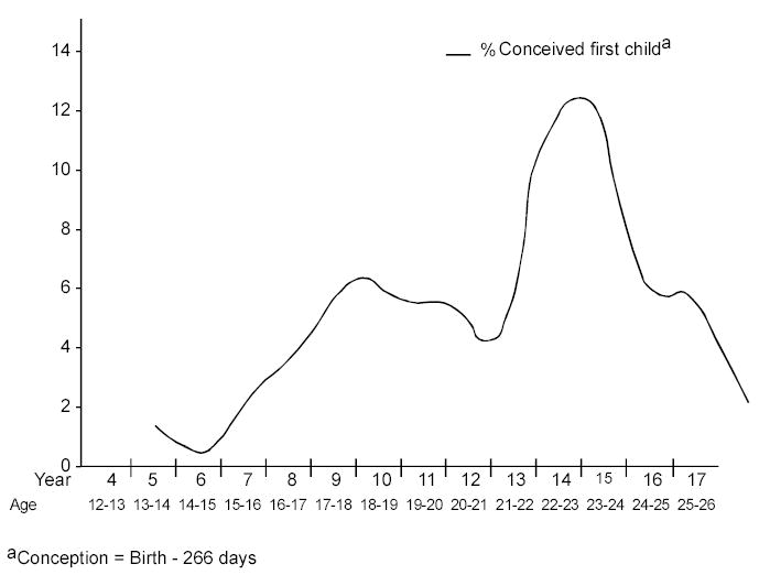
Sample hazard plot for conception of first live birth.

Figure 2b.

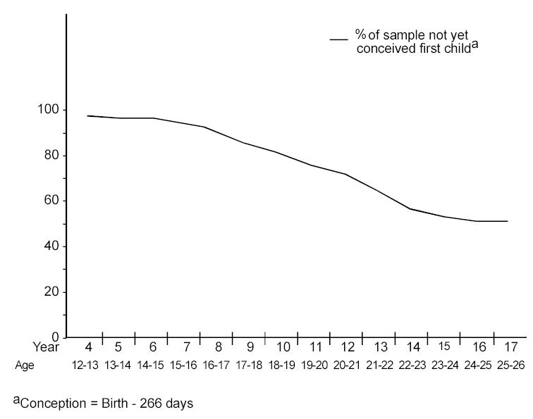
Sample survival plot for conception of first live birth.

Discrete Time Survival Analyses

Univariate analyses

Before conducting the multivariate survival analysis, univariate analyses were completed (Table 2, first column). For each variable, a logistic regression was performed predicting conception wherein the dummy time variables were entered first, followed by the one specific independent variable being considered. Lastly, a set of variables representing the interactions between the dummy time variables and the univariate predictor in question was entered to test whether the effects of each predictor were constant over time. In all of these univariate tests, as hypothesized, the factors significantly predicted timing of fatherhood at the .05 level. When the interaction of each predictor with time was tested, contrary to hypotheses, only the interaction between time and frequency of intercourse was significant. Thus, this interaction was entered as a last step in the multivariate analysis.

Table 2.

Three-Step Regression Models of the Timing of First Fatherhood on Familial, Individual, and Proximal Factors

	Univariate		Model 1		Model 2		Model 3
Predictor	B	Exp B	B	Exp B	B	Exp B	B	Exp B
Familial Risk Factors
Mother’s age at first birth	−0.12	0.89**	−0.08	0.92**	−0.07	0.93*	−0.09	0.92*
Family-of-Origin SES	−0.44	0.64**	−0.30	0.74*	−0.28	0.76*	−0.48	0.62**
Transitions to age 12 years	0.15	1.16**	0.07	1.07	0.06	1.06	0.04	1.04
Parental monitoring	−0.40	0.67**	−0.29	0.75*	−0.04	0.97	0.09	1.10
Individual Problem Behaviors
Academic skill	−0.65	0.52**			−0.41	0.67*	−0.38	0.68*
Antisocial behavior and associations	0.45	1.57**			0.08	1.08	0.11	1.12
Substance use	0.42	1.53**			0.34	1.41**	0.19	1.21
Proximal Factors
Relationship status	2.17	8.80**					1.65	5.20**
Frequency of intercourse	0.01	1.01**					0.002	1.00
Number of sexual partners	0.04	1.04*					0.01	1.01
Failure to use condoms	0.47	1.60*					0.27	1.30**
Block X2			33.54**		17.30**		95.42**
Nagelkerke R2			0.86		0.86		0.89

Note: The time variables that are included in the analyses are not included in the table.

^*p < .05.

^**p < .01.

Multivariate analyses

Hierarchical logistic regressions were used to test the effects of variables in four blocks, namely the dummy coded time variables, followed by the familial, individual problem behavior, and proximal risk factors (Table 2). First, the dummy coded time variables were entered to estimate the baseline hazard function of the conception of the first live birth. All time variables were significant, and the block and model were significant (χ² = 2160.85, [13, N = 2118] p < .001).

The block of familial risk factors was significant (χ² = 33.54, [4, N = 2118] p < .001). Within the block, as hypothesized, age of the youth’s mother at the birth of her first child, family-of-origin SES, and parental monitoring in the family of origin were significant predictors. Examination of the exponentiated beta indicated that a 1-year increase in the age of the youth’s mother at the birth of her first child reduced the baseline odds of conceiving a child by 8% (1 -[exp] B; .92). An increase of one standard deviation in the youth’s parents’ SES level reduced the odds of conception of the first live birth by 26.1%, and an increase of one standard deviation in the parents’ monitoring of the youth reduced the odds by a similar proportion (25.3%).

Next, individual problem behaviors were entered as a block (χ² = 17.30 [3, N = 2118] p < .001). Having good academic skills significantly reduced the odds of fathering by 33.4% for each increase of one standard deviation, whereas each one-unit increase in substance use frequency significantly increased the odds by 40.4%. Contrary to hypotheses, antisocial behavior and associations was not significant in the multivariate model. As predicted, parental monitoring in the family of origin ceased to be a significant predictor in the presence of the individual problem behavior factors, whereas low SES and mother’s age at the birth of her first child were still significant.

At the next step, the block of proximal risk behaviors was significant (χ² = 95.54 [4, N = 2118] p < .001). As predicted, both relationship status and the failure to use condoms were significant predictors, increasing the odds of fathering a first child by 421% and 30%, respectively. Contrary to hypotheses, frequency of intercourse and number of partners were not significant predictors.

Although the main effect for frequency of intercourse was not significant, the block of time by frequency of intercourse terms was entered into the model in a final step because it had been significant in univariate analyses. The significant chi-square for the block (χ² = 28.54 [5, N = 2118] p < .01) indicated that the effects of frequency of intercourse were not constant over time. Inspection of the individual interaction terms indicated that there were only two time points at which there appeared to be significant interactions, Year 5 (ages 13–14; β = .62, Exp β = 1.86, p < .01) and Year 10 (ages 20–21; β = .04, Exp β = 1.04, p < .05). At Year 5, very few youths were engaging in intercourse at all. The three youths who fathered their first child in that year had the highest rates of intercourse. Thus, it appears that having any intercourse at all put youths at higher risk for pregnancy in that year.

At Year 10, the interaction effect appears to be attributable to the way in which frequency of intercourse was coded. As explained in the methods section, in Years 9 – 11, the categorical responses to the question about frequency of intercourse were recoded to the middle point of each category. In Year 10, 9 of the 10 men who fathered children selected the highest category of frequency of intercourse; thus, all were recoded to the same value. The resultant loss of variability for these men appears to have artificially inflated the effect of frequency of intercourse for that year, resulting in the significant interaction term. To test that this did not affect the other findings, frequency of intercourse and number of sexual partners were recoded into categorical variables at each time point. Patterns of significance in those results did not differ from those presented here; thus continuous variables were retained in the final analyses.

In the final model, age of mother at first birth, parental SES, and academic skills, in addition to relationship status and failure to use condoms, remained significant. Therefore, prediction from substance use was explained by the more proximal risk factors. The values of the Nagelkerke R² (Table 2) do not appear to vary much across the three blocks of predictors. This is because the block of time variables (not shown) accounted for a majority of the variance. Overall, in terms of interactions of the predictors with time, the analyses showed, as hypothesized, that the effects of most predictors, with the exception of frequency of intercourse, were constant across time. Contrary to hypotheses, however, the effects of parental monitoring also appeared to be constant across time.

Discussion

The timing of first fatherhood was examined for young men in their mid-20s who were at risk for the development of antisocial behavior by virtue of having lived in higher crime neighborhoods as children. By ages 25 – 26 years, one half of the young men were fathers. A model was proposed in which antisocial behavior was central to risk for early-timed parenthood because it is a marker for, as well as key contributor to, developmental failures and early role transitions that increase risk for further off-time role transitions. We posited that contextual risk in the family of origin would lead to increased risk for problem behaviors, which in turn would lead to earlier engagement in sexual behaviors as well as serious relationships, setting the stage for early entry into fatherhood. Antisocial behavior and peer associations and the difficulties that arise from such behavior were thus posited to lead both directly and indirectly to earlier transitions to fatherhood.

Although all the predictors individually were associated significantly with the timing of entry into fatherhood, the findings of the multivariate prediction model were relatively complex. The effects of familial risk appeared to operate directly and indirectly on timing of fatherhood . As predicted, the age of the youth’s mother when she had her first child continued to be predictive of timing of fathering, even when more proximal variables were entered into the event history model, arguing for a strong intergenerational effect of the timing of parenthood. This effect does not seem to be due either to poor supervision by younger parents, because mother’s age accounted for unique variance even when parental monitoring was in the model, or to the fact that young parents may have fewer educational and occupational opportunities, as the effect persisted when family SES and academic skill were in the equation. Early parenthood may appear normative to children born to young parents.

That family-of-origin SES was predictive of timing of fatherhood is consistent with hypotheses and results of studies of adolescent fathering: SES predicts fathering even when characteristics such as the youth’s antisocial behaviors are accounted for (Fagot et al., 1998; Thornberry et al., 1997). Perhaps the persistence of this effect across time is because of having been raised in a particular class culture in which the norms about timing of the transition into parenthood differ from that of middle-class culture. White, working-class families tend to begin childbearing earlier than middle-class families (Forste, 2002), and parental SES, most notably parental educational attainment, is positively associated with adolescents’ expectations of later entry into adult roles (Crockett & Bingham, 2000). Additionally, youths from lower SES backgrounds may perceive themselves as having fewer educational and income opportunities. Thus, they may not take the steps to prevent parenthood that a youth with greater opportunities might take (Hanson et al., 1989). Youths with plans for higher education do perceive the normative age for entry into parenthood as later than do youths without such plans (Crockett & Bingham, 2000; East, 2000).

Parental monitoring appeared to have the hypothesized indirect effect on timing of fatherhood. It was predictive when the familial risk factors were entered alone into the equation, but the effects were attenuated when the individual risk factors were entered. Antisocial behavior and substance use are highly associated with poor parental supervision (Chilcoat et al., 1995; Patterson & Stouthamer-Loeber, 1984). Thus, poor monitoring may well have its effect on timing of fatherhood because it heightens youths’ risk for these antisocial behaviors.

We hypothesized that individual problem behaviors would be strongly related to timing of fatherhood, both directly and through their effects on sexual and relationship behaviors. Poor academic skills consistently have been associated with a number of early transitions, including early parenthood (Fagot et al., 1998; Gest al., 1999; Scaramella et al., 1998; Thornberry et al., 1997). Youths who fail academically may have fewer prospects for higher education and high occupational attainment. Thus, they may be less likely to postpone parenthood. At least one study has linked poor grades in school to earlier expected timing of role transitions in adolescents (Crockett & Bingham, 2000). Becoming a father may be viewed as an adult behavior that can be successfully accomplished. The youth’s academic skills in adolescence continued to affect life course transitions well into young adulthood, when young men with higher academic skills continued to postpone fatherhood.

Substance use was associated with timing of fathering in the absence of measures of proximal behaviors, but ceased to predict unique variance once these measures were added to the model. Substance use was strongly associated with number of sexual partners and failure to use condoms. Thus, substance use may lead to riskier sexual behaviors (Capaldi et al., 2002), in turn increasing the risk of pregnancy. Antisocial behavior and associations, a construct that has been associated with early fatherhood in other studies (e.g., Jaffee at al., 2001), was predictive of earlier entry into fatherhood in univariate but not in multivariate analyses. This may be partially because of its strong associations with substance use and academic failure. Thus, the analyses did not support the model that antisocial behavior is a key factor in early entry into fatherhood. Rather behaviors that are strongly associated with antisocial behavior, notably failure to succeed in school, a key developmental task that sets the stage for adult role transitions, were more predictive of fathering.

A key contribution of the current study was to examine the effects of being in a committed relationship and of sexual risk behaviors on prediction of fatherhood. As expected, the failure to use condoms predicted earlier entry into fatherhood. This confirms the importance of condoms in prevention of pregnancy at younger ages. It was surprising that neither number of sexual partners nor frequency of intercourse predicted timing of fatherhood in the multivariate survival analysis as both are risk factors for pregnancy and both were significant predictors in the univariate analyses. The sexual behavior variables were fairly strongly interrelated, however, and associated with length of relationship. Thus, condom use and length of relationship (discussed below) may have accounted for the majority of the association.

Being in a committed relationship increased the likelihood of fathering across all ages. Cohabitation and marriage might be expected to increase the chances of parenthood; there are ongoing opportunities for sexual contact and such couples often want to start a family. In this study, many men became fathers in adolescence, when they might not be expected to be in a lengthy relationship. Posthoc analyses examined the length of the young men’s relationships with the mothers of their children prior to the children’s births. Men who became fathers between ages 14 and 21 years had significantly shorter relationships (M = 20.17 mos, SD = 13.29) than did men who became fathers after age 21 years (M = 36.90 mos, SD = 26.60), F(1, 98) = 17.61, p < .001. That the average length of relationship for the younger fathers was 20 months suggests that many of them had relationships of almost a year before the conception of the child. Almost one half of even the very youngest fathers (aged 14 to 17 years) had been in a relationship with the mother of their child for a year or more before their children’s births. At least some of the early fathers may be following the traditional path to adulthood in the sense of engaging in a lengthy courtship before having a child and, even though they are more likely to be engaged in problem behaviors, they may be trying to succeed in the areas of procreation and family formation. Marriage alone did not seem to affect fertility as results did not differ when the partner status variable denoted whether the couple was married (vs. cohabitating or dating) or whether the couple was married or cohabitating (vs. dating).

A further aim of the study was to determine whether the effects of the predictors varied across ages. In the survival analyses, the sole interaction effect between time and frequency of intercourse suggested that this predictor was more important for the youngest fathers (ages 13 –14 years). Overall, these findings suggest that rather than being associated only with very early or adolescent fatherhood in at-risk men, these risk factors continue to predict even as the timing becomes more normative in the mid-20s. This is consistent with prior studies. Jaffee et al. (2001) showed that both familial risk factors and individual problem behaviors predicted the timing of fatherhood through the mid-20s, and Gest et al. (1999) found that adolescent parents and youth who became parents in their early 20s shared similar risk factors.

Limitations of the Study

These findings should be considered in relation to the sample characteristics. This was a sample of predominantly lower SES, White young men who were at-risk for antisocial behavior because they were raised in high-crime neighborhoods. Many previous studies of the timing of fathering have focused on middle- to upper-middle-class samples (Forste, 2002); thus, the current study makes a valuable contribution to the literature. The generalizability of the findings, however, particularly to men of other SES and ethnic groups, needs to be established. Further, the inclusion of a group of men not at risk for antisocial behavior would help to establish whether the model is applicable to young men in general. Finally, this sample was relatively young because the men were only in their mid-20s at the latest year of the study. A sample with a greater range of ages might help to shed light on the factors that contribute to later fathering.

Directions for Future Research

Future research should explore how the characteristics predictive of entry into fatherhood are linked to men’s attitudes about reproduction, family formation, and expectancies about the timing of role transitions. As noted above, some researchers have suggested that lower SES may be linked to early parenting because these youths believe that they have reduced opportunities for economic advancement and thus do not delay parenthood (Hanson et al., 1989). Whereas the results of the current study support past findings that lower SES is linked to earlier fatherhood, the reasons for this association are not clear. Research linking attitudes, sexual behaviors, and plans for family formation would help to clarify these associations. Given that these youths were selected for the sample because they lived in high-crime neighborhoods, future work should explore whether norms about the timing of first sexual experiences and parenting differ in such neighborhoods. There is a large literature demonstrating that neighborhood characteristics can influence the sexual and reproductive behaviors of adolescents but most focus on the racial and SES composition of neighborhoods (e.g., Ku, Sonenstein, & Pleck, 1993; South & Baumer, 2000). Further work on how neighborhood crime might influence these processes is warranted.

This study suggests that the inability to master key developmental tasks—such as school achievement—does lead to early entry into at least one adult role. It also adds to a growing consensus that preventing problem behaviors and school failure as well as promoting consistent condom use may help prevent early fatherhood (Fagot et al., 1998; Gest et al., 1999; Thornberry et al., 1997). Additionally, many of the young fathers enter a committed relationship prior to parenthood, suggesting that in spite of their precocity, they are following a traditional path to some degree. Thus, once they do become fathers, it is of paramount importance to support them through training in parenting, relationship, and job skills to help them succeed in that role.

References

- Achenbach, T. M. (1991). Manual for the Child Behavior Checklist/4–18 and 1991 Profile Burlington, VT: University of Vermont, Department of Psychiatry.
- Achenbach, T. M. (1997). Manual for the Young Adult Self-Report and Young Adult Behavior Checklist Burlington, VT: University of Vermont, Department of Psychiatry.
- Achenbach, T. M., & Edelbrock, C. (1983). Manual for the Child Behavior Checklist and Revised Child Behavior Profile Burlington, VT: University of Vermont, Department of Psychiatry.
- Becker PT. Sensitivity to infant development and behavior: A comparison of adolescent and adult single mothers. Research in Nursing and Health. 1987;10:119–127. doi: 10.1002/nur.4770100303. [DOI] [PubMed] [Google Scholar]
- Berlin LJ, Brady-Smith C, Brooks-Gunn J. Links between childbearing age and observed maternal behaviors with 14-month-olds in the early head start research and evaluation project. Infant Mental Health Journal. 2002;23:104–129. [Google Scholar]
- Black MM, Papas MA, Hussey JM, Dubowitz H, Kotch JB, Starr RH., Jr Behavior problems among preschool children born to adolescent mothers: Effects of maternal depression and perceptions of partner relationships. Journal of Clinical Child and Adolescent Psychology. 2002;31:16–26. doi: 10.1207/S15374424JCCP3101_04. [DOI] [PubMed] [Google Scholar]
- Burton, L. M., Obeidallah, D. A., & Allison, K. (1996). Ethnographic insights on social context and adolescent development among inner-city African-American teens. In R. Jessor, A. Colby, & R. A. Shweder (Eds.), Ethnography and human development: Context and meaning in social inquiry (pp. 395–418). Chicago: University of Chicago Press.
- Capaldi DM. The co-occurrence of conduct problems and depressive symptoms in early adolescent boys: II. A 2-year follow-up at Grade 8. Development and Psychopathology. 1992;4:125–144. doi: 10.1017/s0954579499001959. [DOI] [PubMed] [Google Scholar]
- Capaldi DM, Crosby L, Stoolmiller M. Predicting the timing of first sexual intercourse for at-risk adolescent males. Child Development. 1996;67:344–359. [PubMed] [Google Scholar]
- Capaldi, D. M., King, J., & Wilson, J. (1992). Young Adult Adjustment Scale Unpublished OSLC instrument. (Available from OSLC, 160 E. 4th, Eugene, OR 97401.)
- Capaldi DM, Patterson GR. Relation of parental transitions to boys’ adjustment problems: I. A linear hypothesis. II. Mothers at risk for transitions and unskilled parenting. Developmental Psychology. 1991;27:489–504. [Google Scholar]
- Capaldi, D. M., & Patterson, G. R. (1994). Interrelated influences of contextual factors on antisocial behavior in childhood and adolescence for males. In D. Fowles, P. Sutker, & S. Goodman (Eds.), Progress in experimental personality and psychopathology research (pp. 165–198). New York: Springer. [PubMed]
- Capaldi DM, Pears KC, Patterson GR, Owen LD. Continuity of parenting practices across generations in an at-risk sample: A prospective comparison of direct and mediated associations. Journal of Abnormal Child Psychology. 2003;31:127–142. doi: 10.1023/a:1022518123387. [DOI] [PubMed] [Google Scholar]
- Capaldi, D. M., & Shortt, J. W. (2003). Understanding conduct problems in adolescence from a lifespan perspective. In G. R. Adams & M. D. Berzonsky (Eds.), Blackwell handbook of adolescence (pp. 470–493). Oxford, UK: Blackwell.
- Capaldi DM, Stoolmiller M, Clark S, Owen LD. Heterosexual risk behaviors in at-risk young men from early adolescence to young adulthood: Prevalence, prediction, and STD contraction. Developmental Psychology. 2002;38:394–406. doi: 10.1037//0012-1649.38.3.394. [DOI] [PubMed] [Google Scholar]
- Chilcoat H, Dishion TJ, Anthony JC. Parent monitoring and the incidence of drug sampling in urban elementary school children. American Journal of Epidemiology. 1995;141:25–31. doi: 10.1093/oxfordjournals.aje.a117340. [DOI] [PubMed] [Google Scholar]
- Cicchetti D, Rogosch FA. A developmental psychopathology perspective on adolescence. Journal of Consulting and Clinical Psychology. 2002;70:6–20. doi: 10.1037//0022-006x.70.1.6. [DOI] [PubMed] [Google Scholar]
- Cooney TM, Pedersen FA, Indelicato S, Palkovitz R. Timing of fatherhood: Is “on-time” optimal? Journal of Marriage and the Family. 1993;55:205–215. [Google Scholar]
- Crockett LJ, Bingham CR. Anticipating adulthood: Expected timing of work and family transitions among rural youth. Journal of Research on Adolescence. 2000;10:151–172. [Google Scholar]
- Dishion TJ. The family ecology of boys’ peer relations in middle childhood. Child Development. 1990;61:874–892. doi: 10.1111/j.1467-8624.1990.tb02829.x. [DOI] [PubMed] [Google Scholar]
- Dishion, T. J., & Capaldi, D. M. (1985). Peer Involvement and Social Skills Questionnaire Unpublished OSLC instrument. (Available from OSLC, 160 E. 4th, Eugene, OR 97401.)
- East PL. Racial and ethnic differences in girls’ sexual, marital and birth expectations. Journal of Marriage and the Family. 1998;60:150–162. [PMC free article] [PubMed] [Google Scholar]
- Elliott, D. S., & Voss, H. L. (1974). Delinquency and dropout Lexington, MA: Lexington Books.
- Elliott, D. S., Ageton, S. S., Huizinga, D., Knowles, B. A., & Canter, R. J. (1983). The prevalence and incidence of delinquent behavior: 1976–1980. National estimates of delinquent behavior by sex, race, social class, and other selected variables (National Youth Survey Report No. 26) Boulder, CO: Behavioral Research Institute.
- Fagot BI, Pears KC, Capaldi DM, Crosby L, Leve CS. Becoming an adolescent father: Precursors and parenting. Developmental Psychology. 1998;34:1209–1219. doi: 10.1037//0012-1649.34.6.1209. [DOI] [PubMed] [Google Scholar]
- Forste R. Where are all the men?: A conceptual analysis of the role of men in family formation. Journal of Family Issues. 2002;23:579–600. [Google Scholar]
- Gest SD, Mahoney JL, Cairns RB. A developmental approach to prevention research: Configural antecedents of early parenthood. American Journal of Community Psychology. 1999;27:543–565. doi: 10.1023/A:1022185312277. [DOI] [PubMed] [Google Scholar]
- Goodyear RK, Newcomb MD, Allison RD. Predictors of Latino men’s paternity in teen pregnancy: Test of a mediational model of childhood experiences, gender role attitudes, and behaviors. Journal of Counseling Psychology. 2000;47:116–128. [Google Scholar]
- Gottfredson, M. R., & Hirschi, T. (1990). A general theory of crime Stanford, CA: Stanford University Press.
- Hanson SL, Morrison DR, Ginsburg AL. The antecedents of teenage fatherhood. Demography. 1989;26:579–596. [PubMed] [Google Scholar]
- Hardy JB, Astone NM, Brooks-Gunn J, Shapiro S, Miller TL. Like mother, like child: Intergenerational patterns of age at first birth and associations with childhood and adolescent characteristics and adult outcomes in the second generation. Developmental Psychology. 1998;34:1220–1232. doi: 10.1037//0012-1649.34.6.1220. [DOI] [PubMed] [Google Scholar]
- Heath TD. The impact of delayed fatherhood on the father-child relationship. Journal of Genetic Psychology. 1994;155:511–530. doi: 10.1080/00221325.1994.9914799. [DOI] [PubMed] [Google Scholar]
- Hill KG, Howell JC, Hawkins JD, Battin-Pearson SR. Childhood risk factors for adolescent gang membership: Results from the Seattle Development Project. Journal of Research in Crime and Delinquency. 1999;36:300–322. [Google Scholar]
- Hogan DP, Astone NM. The transition to adulthood. Annual Review of Sociology. 1986;12:109–130. [Google Scholar]
- Hollingshead, A. B. (1975). Four factor index of social status. Unpublished manuscript, Yale University, New Haven, CT.
- Ingoldsby E, Shaw DS. Neighborhood contextual factors and early-starting antisocial pathways. Clinical Child and Family Psychology Review. 2002;5:21–55. doi: 10.1023/a:1014521724498. [DOI] [PubMed] [Google Scholar]
- Jaffee SR, Caspi A, Moffitt TE, Taylor A, Dickson N. Predicting early fatherhood and whether young fathers live with their children: Prospective findings and policy reconsiderations. Journal of Child Psychology and Psychiatry. 2001;42:803–815. doi: 10.1111/1469-7610.00777. [DOI] [PubMed] [Google Scholar]
- Kessler RC, Crum RM, Warner LA, Nelson CB, Schulenberg J, Anthony JC. Lifetime co-occurrence of DSM-III-R alcohol abuse an dependence with other psychiatric disorders in the National Comorbidity Survey. Archives of General Psychiatry. 1997;54:313–321. doi: 10.1001/archpsyc.1997.01830160031005. [DOI] [PubMed] [Google Scholar]
- Ku L, Sonenstein FL, Pleck JH. Neighborhood, family, and work: Influences on the premarital behaviors of adolescent males. Social Forces. 1993;72:479–503. [Google Scholar]
- Lerman, R. I. (1993). A national profile of young unwed fathers. In R. I. Lerman & T. Ooms (Eds.), Young unwed fathers: Changing roles and emerging policies (pp. 27–51). New York: Wiley.
- Marini MM. The order of events in the transition to adulthood. Sociology of Education. 1984;57:63–84. [Google Scholar]
- Metzler CW, Noell J, Biglan A, Ary D, Smolkowski K. The social context for risky sexual behavior among adolescents. Journal of Behavioral Medicine. 1994;17:419–438. doi: 10.1007/BF01858012. [DOI] [PubMed] [Google Scholar]
- Miller KS, Forehand R, Kotchick BA. Adolescent sexual behavior in two ethnic minority samples: The role of family variables. Journal of Marriage and the Family. 1999;61:85–98. [Google Scholar]
- Neugarten BL, Moore JW, Lowe JC. Age norms, age constraints, and adult socialization. American Journal of Sociology. 1965;70:710–717. doi: 10.1086/223965. [DOI] [PubMed] [Google Scholar]
- Newcomb MD, McGee L. Influence of sensation seeking on general deviance and specific problem behaviors from adolescence to young adulthood. Journal of Personality and Social Psychology. 1991;61:614–628. doi: 10.1037//0022-3514.61.4.614. [DOI] [PubMed] [Google Scholar]
- Norusis, M. J. (1997). SPSS professional statistics 7.5 Chicago: SPSS.
- Patterson GR, Bank L. Bootstrapping your way in the nomological thicket. Behavioral Assessment. 1986;8:49–73. [Google Scholar]
- Patterson GR, Stouthamer-Loeber M. The correlation of family management practices and delinquency. Child Development. 1984;55:1299–1307. [PubMed] [Google Scholar]
- Sampson RJ. Collective regulation of adolescent misbehavior: Validation results from eighty Chicago neighborhoods. Journal of Adolescent Research. 1997;12:227–244. [Google Scholar]
- Scaramella LV, Conger RD, Simons RL, Whitbeck LB. Predicting risk for pregnancy by late adolescence: A social contextual perspective. Developmental Psychology. 1998;34:1233–1245. doi: 10.1037//0012-1649.34.6.1233. [DOI] [PubMed] [Google Scholar]
- Seidman E, Yoshikawa H, Roberts A, Chesir-Teran D, Allen L, Friedman JL, et al. Structural and experiential neighborhood contexts, developmental stage, and antisocial behavior among urban adolescents in poverty. Development and Psychopathology. 1998;10:259–281. doi: 10.1017/s0954579498001606. [DOI] [PubMed] [Google Scholar]
- Simcha-Fagan O, Schwartz JE. Neighborhood and delinquency: An assessment of contextual effects. Criminology. 1986;24:667–699. [Google Scholar]
- Singer JD, Willett JB. It’s about time: Using discrete-time survival analysis to study duration and the timing of events. Journal of Educational Statistics. 1993;18:155–195. [Google Scholar]
- South SJ, Baumer EP. Deciphering community and race effects on adolescent premarital childbearing. Social Forces. 2000;78:1379–1408. [Google Scholar]
- Stouthamer-Loeber M, Loeber R, Wei EH, Farrington DP, Wikstrom POH. Risk and promotive effects in the explanation of persistent serious delinquency in boys. Journal of Consulting and Clinical Psychology. 2002;70:111–123. doi: 10.1037//0022-006x.70.1.111. [DOI] [PubMed] [Google Scholar]
- Stouthamer-Loeber M, Wei EH. The precursors of young fatherhood and its effect on delinquency of teenage males. Journal of Adolescent Health. 1998;22:56–65. doi: 10.1016/S1054-139X(97)00211-5. [DOI] [PubMed] [Google Scholar]
- Thornberry TP, Smith CA, Howard GJ. Risk factors for teenage fatherhood. Journal of Marriage and the Family. 1997;59:505–522. [Google Scholar]
- Upchurch DM, McCarthy J. The timing of a first birth and high school completion. American Sociological Review. 1990;55:224–234. [Google Scholar]
- U. S. Census Bureau. (2002). Number, timing, and duration of marriages and divorces: 1996 Washington, DC: U.S. Department of Commerce, Economics and Statistics Administration.
- Walker, H. M., & McConnell, S. R. (1988). The Walker-McConnell Scale of Social Competence and School Adjustment Austin, TX: Pro-Ed.
- Willett JB, Singer JD. Investigating onset, cessation, relapse, and recovery: Why you should, and how you can, use discrete-time survival analysis to examine event occurrence. Journal of Consulting and Clinical Psychology. 1993;61:952–965. doi: 10.1037//0022-006x.61.6.952. [DOI] [PubMed] [Google Scholar]
- Xie H, Cairns BD, Cairns RB. Predicting teen motherhood and teen fatherhood: Individual characteristics and peer affiliations. Social Development. 2001;10:488–511. [Google Scholar]