From Quantitative Microscopy to Automated Image Understanding

Abstract

Quantitative microscopy has been extensively used in biomedical research and has provided significant insights into structure and dynamics at the cell and tissue level. The entire procedure of quantitative microscopy is comprised of specimen preparation, light absorption/reflection/emission from the specimen, microscope optical processing, optical/electrical conversion by a camera or detector, and computational processing of digitized images. Although many of the latest digital signal processing techniques have been successfully applied to compress, restore, and register digital microscope images, automated approaches for recognition and understanding of complex subcellular patterns in light microscope images have been far less widely used. In this review, we describe a systematic approach for interpreting protein subcellular distributions using various sets of Subcellular Location Features (SLF) in combination with supervised classification and unsupervised clustering methods. These methods can handle complex patterns in digital microscope images and the features can be applied for other purposes such as objectively choosing a representative image from a collection and performing statistical comparison of image sets.

1. Introduction

Biomedical research has been revolutionized by the new types of information generated from various “omics” projects, beginning with the genome sequencing projects. The genome drafts completed so far have enabled us, for the first time, to discover and compare all possible genes in a number of organisms. To uncover proteome differences in a given organism, expression arrays and protein chips have been used to study the transcription and expression characteristics of all possible proteins in different tissues, at different developmental stages, and under various disease types [1, 2]. High-throughput pipelines in structural proteomics have automated protein structure determination by integrating target purification, crystallization, data acquisition, and final assignment [3]. Location proteomics, one of the latest subfields of proteomics, has the goal of providing an exact description of the subcellular distribution for each protein in a given cell type [4-7]. All of these methods provide valuable information for determining how a protein functions and how its functioning is regulated.

Knowledge of a protein's subcellular distribution can contribute to a complete understanding of its function in a number of different ways. The normal subcellular distribution of a protein provides a scope for its function. For instance, a protein localized in the mitochondrial membrane can be inferred to function in energy metabolism. If a protein has a close subcellular localization pattern to a known protein, there exists a high chance that they form a functional complex protein. The dynamic properties of protein subcellular distribution under different environmental conditions can also provide important information about protein function. If a protein changes its subcellular location from cytoplasm to cell nucleus after treating the cell with a certain drug, it suggests that the protein might play an important role in signal transduction and possibly work as a transcription factor directly.

The current widespread application of biomedical optics was made possible by the invention of quantitative optical instruments. When the microscope was invented more than 300 years ago, the analog signal reflected from the specimen had to be recorded by hand-drawing. The development of cameras permitted creation of still microscope images, but visual inspection was still the only way to interpret results generated from a microscope at that time. After the invention of the digital camera and other optical detectors, the analog signal from a microscope could be recorded at high density in digital media. With the application of digital signal processing techniques, automated analysis of microscope images, which could only be imagined before, became possible. For example, pioneering work on numerical description of microscope image patterns was done for chromosome distributions [8, 9]. The goal of the work reviewed below has been to develop automated methods applicable to all major subcellular patterns.

2. Quantitative Fluorescence Microscopy and Location Proteomics

Compared to other approaches for determining protein subcellular location such as electron microscopy and subcellular fractionation, fluorescence microscopy permits rapid collection of images with excellent resolution between cell compartments. These properties, along with the high specificity methods for targeting fluorescent probes to specific proteins, make fluorescence microscopy the optimal choice for studying the subcellular distribution of a proteome. The choice of different fluorescence microscopy methods, however, depends on the application. Obviously, the signal to noise ratio is the most important factor in using quantitative fluorescence microscopy. The noise in fluorescence microscopy mostly comes from out-of-focus fluorescence and quantization errors in the camera [10]. Although the second source can be reduced dramatically by using expensive CCD cameras, out-of-focus fluorescence is handled differently by different fluorescence microscope systems [10, 11]. Inexpensive widefield microscope systems collect fluorescence emitted from the entire 3D specimen in the field of view, requiring computational removal of out-of-focus fluorescence (deconvolution) after image collection. Deconvolution can be computationally costly and requires an accurate model of the point-spread function for a particular microscope. Confocal laser scanning microscopes collect fluorescence from individual, small regions of the specimen illuminated by a laser scanning beam. Out-of-focus fluorescence is removed by employing a pinhole on the light collection path. Compared to widefield microscopes, confocal laser scanning microscopes have a much lower acquisition rate, but no deconvolution is normally needed. A variation of the confocal laser scanning microscope, the spinning disk confocal microscope, circumvents the speed limit by using a rotating pinhole array which enables fast focusing and image collection. For thin specimens, widefield microscopes perform best; while for thick specimen, it is recommended to use a confocal laser scanning microscope [10]. Fully automated microscopes also have tremendous promise for acquiring the large numbers of images required for systematic analysis of subcellular patterns [12].

To collect fluorescence microscope images of a target protein, two methods are typically used to add a fluorescence tag to a protein of interest. Immunofluorescence employs antibodies that specifically bind to a target protein. It is not suitable for live cell imaging because cells need to be fixed and permeabilized before antibodies can enter. Fluorescence dyes can be bound directly to antibodies, or to secondary antibodies directed against the primary antibodies. The other method is gene tagging, of which there are many variant approaches [13-17]. A particularly useful approach is CD-tagging, which introduces a DNA sequence encoding a fluorescent protein such as GFP into an intron of a target gene. Gene tagging can also be applied randomly throughout a genome without targeting a specific protein, with the assumption that the probabilities of inserting the DNA tag into all genes are roughly equal. For a given cell type, random gene tagging coupled with high-throughput fluorescence microscopy can generate images depicting the subcellular location patterns of all or most expressed proteins. We coined the term location proteomics to describe the combination of tagging, imaging and automated image interpretation to enable proteome-wide study of subcellular location [5].

The necessity of having an automated analysis system stems from need for an objective approach that generates repeatable analysis results, a high-throughput method that can analyze tens of thousands of images per day, and lastly, for a more accurate approach than visual examination. In the following sections, we first describe numerical features that can be used to capture the subcellular patterns in digital fluorescence microscope images. Summaries of feature reduction and classification methods are discussed next. (These sections can be skipped by readers primarily interested in learning the types of automated analyses that can be carried out on microscope images.) We then evaluate the image features for the tasks of supervised classification and unsupervised clustering by using various image datasets collected in our group and from our colleagues. Lastly, we describe a few other uses of image features in practical biomedical research.

3. Automated Interpretation of Images

3.1 Image Features

Given a combination of a protein expression level, a tagging approach, and a microscope system that yields a sufficiently high signal-to-noise ratio, we can obtain a precise digital representation of the subcellular location pattern of that protein. The next step, automated interpretation of that pattern, requires extracting informative features from the images that represent subcellular location patterns better than the values of the individual pixels. We have therefore designed and implemented a number of feature extraction methods for single cell images [5, 18-20]. To be useful for analyzing cells grown on a slide, cover slip or dish, we require that these features be invariant to translation and rotation of the cell in the plane of the microscope stage and robust across different microscopy methods and cell types.

One approach to developing features for this purpose is to computationally capture the aspects of image patterns that human experts describe. We have used a number of features of this type, especially those derived from morphological image processing. An alternative, however, is to use less intuitive features which seek a more detailed mathematical representation of the frequencies present in an image and its gray level distribution. These features capture information that a human observer may neglect and may allow an automated classifier to perform better than a human one. We have therefore used features of this type, such as texture measures, as well.

The feature extraction methods we have used are described briefly below for 2D and/or 3D single cell images.

3.1.1 2D Features:

3.1.1.1 Zernike Moment Features

A filter bank of Zernike polynomials can be used to describe the gray-level pixel distribution in each fluorescence microscope image [21]. An image to be analyzed is first transformed to the unit circle by subtracting the coordinates of the center of fluorescence from those of each pixel and dividing all coordinates by a user-specified cell radius r. A Zernike moment is calculated as the correlation between the transformed image, f (x, y) (x² + y² ≤ 1) , and a specific Zernike polynomial. The magnitude of the Zernike moment is used as a feature describing the similarity of the gray-level pixel distribution of an image to that Zernike polynomial. We calculate 49 Zernike moment features by using the Zernike polynomials up to order 12 [22, 23]. Since an image is first normalized to the unit circle and only the magnitude of Zernike moments is used, this group of features satisfies the requirements of rotation and translation invariance.

3.1.1.2 Haralick Texture Features

Haralick texture features provide statistical summaries of the spatial frequency information in an image [24]. Firstly, a gray-level co-occurrence matrix is generated by calculating the probability that a pixel of each gray level is found adjacent to a pixel of all other gray levels. Given a total number of gray levels N_g in an image, the co-occurrence matrix is N_g × N_g. For 2D images, there are four possible co-occurrence matrixes that measure the pixel adjacency statistics in horizontal, vertical, and two diagonal directions respectively. To satisfy the requirements of rotation and translation invariance, the four matrixes are averaged and used to calculate 13 intrinsic statistics, including angular second moment, contrast, correlation, sum of squares, inverse difference moment, sum average, sum variance, sum entropy, entropy, difference variance, difference entropy, information measure of correlation 1, and information measure of correlation 2 [23]. One restriction of Haralick features is that they are not invariant to the total gray level used as well as the pixel size in an image. To address this, a series of experiments were conducted to find an optimal gray levels and coarsest pixel size for use in HeLa cells under all microscopy conditions [18]. The most discriminative Haralick features were obtained when images were resampled to 1.15 microns/pixel and quantized using 256 gray levels. Resampling to these settings for HeLa cells can be used to calculate Haralick features on a common frame of reference for varying microscope objectives and cameras [18]. Whether this resolution is optimal for other cell types remains to be determined.

3.1.1.3 Wavelet Features

Wavelet transform features can also be used to capture frequency information in an image. To extract features from the wavelet transform of an image, a multi-resolution scheme is often used [25]. An image can be convolved with wavelets of different scales and statistics of the pixel intensity in the resulting images (such as mean, standard deviation, and average energy) are often used as features. Here we describe two sets of recently applied wavelet features derived from the Gabor wavelet transform and the Daubechies 4 wavelet transform (Huang and Murphy, submitted). Since wavelet transforms are not invariant to cell translation and rotation, each image is pivoted at its center of fluorescence and rotated to align its primary axis with the y axis in the image plane before feature extraction. Alignment of the secondary axis can be achieved by conducting an extra 180° rotation if necessary to make the third central moment of x positive.

3.1.1.3.1 Daubechies 4 wavelet features

The Daubechies wavelet family is one of the most frequently used wavelet transforms in image analysis [26]. Each wavelet transform consists of a scale function and a wavelet function, which can be regarded as a low-pass and a high-pass filter respectively [25]. Given the Daubechies 4 wavelet transform with its scale function and wavelet function, an image is sequentially convolved column-wise and row-wise by these two filters respectively. The four convolved images carry different frequency information extracted from the original image. Three of them contain high frequency information in the x, y, and diagonal directions of the original image respectively. The last one contains low frequency information and can be regarded as a smoothed version of the original image. Further decomposition on the smoothed image will give us finer information on lower frequency bands. We used Daubechies 4 wavelet transform to decompose an image up to the 10^th level and the average energies of the three high-frequency images at each level were used as features. In total, 30 wavelet features can be obtained that represent the frequency information in the original image best captured by Daubechies 4 wavelet transform.

3.1.1.3.2 Gabor wavelet features

The Gabor function has been used as an important filtering technique in computer vision since it was found to be able to model receptive field profiles of cortical simple cells [27]. The information captured by the nonorthogonal Gabor wavelet is mostly the derivative information of an image such as edges [28]. A Gabor filter bank can be generated using Gabor filters with different orientations and scales. The mean and standard deviation of the pixel intensity in a convolved image are often used as features, which represent the frequency information in the original image best captured by the Gabor wavelet transform. We have used 60 Gabor wavelet features from a filter bank composed of six different orientations and five different scales (Huang and Murphy, submitted).

3.1.1.4 Morphological Features

Image morphology describes various characteristics of objects, edges, and the entire image such as the average size of each object, the edge intensity homogeneity, and the convex hull of the entire image. Unlike some natural scene images, fluorescence microscope images can be well characterized by their mathematical morphology [18, 19]. Morphological information of an image represents group statistics, intrinsically invariant to cell rotation and translation. The morphological features we have used include fourteen features derived from finding objects (connected components after automated thresholding), five features from edges, and three features from the convex hull of the entire image [18, 19]. Since multi-channel imaging has become routine in fluorescence microscopy, additional channels can be added to improve the recognition of the subcellular location pattern of a target protein. A commonly used reference in our experiments is the distribution of a DNA-binding probe that labels the cell nucleus [19]. The DNA channel image introduces an extra pivot in images for studying protein subcellular location. We have therefore used six additional object features to describe the relative location of the protein channel to the DNA channel.

3.1.1.5 SLF Nomenclature

We have created a systematic nomenclature for referring to the image features used to describe subcellular location patterns, which we term SLF (Subcellular Location Feature) sets [18, 19]. Each set found to be useful for classification or comparison is assigned an SLF set number. Each feature in that set has the prefix “SLF” followed by the set index and the index of the feature in that set. For instance, SLF1.7, which is the variance of object distances from the center of fluorescence, is the seventh feature in feature set SLF1. Table 1 gives a summary of all current 2D features grouped by various feature sets. The features derived from a parallel DNA channel for a target protein are included in the feature sets SLF2, SLF4, SLF5, and SLF13 [18, 19].

Table 1.

Feature sets defined for 2D fluorescence microscope images.

Set	SLF No.	Feature Description
SLF1	SLF1.1	The number of fluorescence objects in the image
	SLF1.2	The Euler number of the image (no. of holes minus no. of objects)
	SLF1.3	The average number of above-threshold pixels per object
	SLF1.4	The variance of the number of above-threshold pixels per object
	SLF1.5	The ratio of the size of the largest object to the smallest
	SLF1.6	The average object distance to the cellular center of fluorescence (COF)
	SLF1.7	The variance of object distances from the COF
	SLF1.8	The ratio of the largest to the smallest object to COF distance
	SLF1.9	The fraction of the non-zero pixels that are along an edge
	SLF1.10	Measure of edge gradient intensity homogeneity
	SLF1.11	Measure of edge direction homogeneity 1
	SLF1.12	Measure of edge direction homogeneity 2
	SLF1.13	Measure of edge direction difference
	SLF1.14	The fraction of the convex hull area occupied by protein fluorescence
	SLF1.15	The roundness of the convex hll
	SLF1.16	The eccentricity of the convex hull
SLF2	SLF2.1-2.16	SLF1.1-SLF1.16
	SLF2.17	The average object distance from the COF of the DNA image
	SLF2.18	The variance of object distances from the DNA COF
	SLF2.19	The ratio of the largest to the smallest object to DNA COF distance
	SLF2.20	The distance between the protein COF and the DNA COF
	SLF2.21	The ratio of the area occupied by protein to that occupied by DNA
	SLF2.22	The fraction of the protein fluorescence that co-localizes with DNA
SLF3	SLF3.1-3.16	SLF1.1-SLF1.16
	SLF3.17-3.65	Zernike moment features
	SLF3.66-3.78	Haralick texture features
SLF4	SLF4.1-4.22	SLF2.1-2.22
	SLF4.23-4.84	SLF3.17-3.78
SLF5	SLF5.1-SLF5.37	37 features selected from SLF4 using stepwise discriminant analysis
SLF6	SLF6.1-6.65	SLF3.1-SLF3.65
SLF7	SLF7.1-7.9	SLF3.1-3.9
	SLF7.10-7.13	Minor corrections to SLF3.10-SLF3.13
	SLF7.14-	SLF3.14-SLF3.65
	SLF7.66-	Haralick texture features calculated on fixed size and intensity scales
	SLF7.79	The fraction of cellular fluorescence not included in objects
	SLF7.80	The average length of the morphological skeleton of objects
	SLF7.81	The average ratio of object skeleton length to the area of the convex hull of the
	SLF7.82	The average fraction of object pixels contained within its skeleton
	SLF7.83	The average fraction of object fluorescence contained within its skeleton
	SLF7.84	The average ratio of the number of branch points in skeleton to length of skeleton
SLF8	SLF8.1-8.32	32 features selected from SLF7 using stepwise discriminant analysis
SLF12	SLF12.1-12.8	SLF8.1-8.8, the smallest feature set able to achieve 80% accuracy
SLF13	SLF13.1-13.31	31 features selected from SLF7 and SLF2.17-2.22 using stepwise discriminant analysis

3.1.2 3D Features

3.1.2.1 3D Morphological Features

As an initial approach to describing the 3D distribution of proteins in cells, we used a direct extension of some of the 2D features to 3D [20]. Converting 2D features that depend on area to 3D counterparts using volume is straightforward. However, because of the asymmetry between the slide plane and the microscope axis, directly converting features measuring 2D distance to 3D distance would lose important information present in 3D image collection. While protein distribution in the plane of the slide can be considered to be rotationally equivalent, the distribution for adherent cells along the microscope axis is not (since some proteins are distributed preferentially near the bottom or top of the cell). The distance computation in 3D images was therefore separated into two components, one in the slide plane and the other along the microscope axis. While 2D edge features can be extended to 3D directly, for computational convenience two new features were designed from 2D edges found in each 2D slice of a 3D image [5]. Table 2 shows all current 3D features.

Table 2.

Feature sets defined for 3D fluorescence microscope images.

Feature Setname	SLF No.	Feature Description
SLF9	SLF9.1	The number of fluorescent objects in the image
	SLF9.2	The Euler number of the image
	SLF9.3	The average object volume
	SLF9.4	The standard deviation of object volumes
	SLF9.5	The ratio of the max object volume to min object volume
	SLF9.6	The average object distance to the protein center of fluorescence (COF)
	SLF9.7	The standard deviation of object distances from the protein COF
	SLF9.8	The ratio of the largest to the smallest object to protein COF distance
	SLF9.9	The average object distance to the COF of the DNA image
	SLF9.10	The standard deviation of object distances from the COF of the DNA image
	SLF9.11	The ratio of the largest to the smallest object to DNA COF distance
	SLF9.12	The distance between the protein COF and the DNA COF
	SLF9.13	The ratio of the volume occupied by protein to that occupied by DNA
	SLF9.14	The fraction of the protein fluorescence that co-localizes with DNA
	SLF9.15	The average horizontal distance of objects to the protein COF
	SLF9.16	The standard deviation of object horizontal distances from the protein COF
	SLF9.17	The ratio of the largest to the smallest object to protein COF horizontal
	SLF9.18	The average vertical distance of objects to the protein COF
	SLF9.19	The standard deviation of object vertical distances from the protein COF
	SLF9.20	The ratio of the largest to the smallest object to protein COF vertical
	SLF9.21	The average object horizontal distance from the DNA COF
	SLF9.22	The standard deviation of object horizontal distances from the DNA COF
	SLF9.23	The ratio of the largest to the smallest object to DNA COF horizontal
	SLF9.24	The average object vertical distance from the DNA COF
	SLF9.25	The standard deviation of object vertical distances from the DNA COF
	SLF9.26	The ratio of the largest to the smallest object to DNA COF vertical distance
	SLF9.27	The horizontal distance between the protein COF and the DNA COF
	SLF9.28	The signed vertical distance between the protein COF and the DNA COF
SLF10	SLF10.1-10.9	9 features selected from SLF9 using stepwise discriminant analysis
SLF11	SLF11.1-11.14	SLF9.1-9.8, SLF9.15-9.20
	SLF11.15	The fraction of above threshold pixels that are along an edge
	SLF11.16	The fraction of fluorescence in above threshold pixels that are along an edge
	SLF11.17/30	Average/range of angular second moment
	SLF11.18/31	Average/range of contrast
	SLF11.19/32	Average/range of correlation
	SLF11.20/33	Average/range of sum of squares of variance
	SLF11.21/34	Average/range of inverse difference moment
	SLF11.22/35	Average/range of sum average
	SLF11.23/36	Average/range of sum variance
	SLF11.24/37	Average/range of sum entropy
	SLF11.25/38	Average/range of entropy
	SLF11.26/39	Average/range of difference variance
	SLF11.27/40	Average/range of difference entropy
	SLF11.28/41	Average/range of info measure of correlation 1
	SLF11.29/42	Average/range of info measure of correlation 2
SLF14	SLF14.1-14.14	SLF9.1-9.8, SLF9.15-9.20

3.1.2.2 3D Haralick Texture Features

Although Haralick texture features were originally designed for 2D images, the idea of extracting pixel adjacency statistics can be easily extended to voxel adjacency in 3D images [5]. Instead of four directional adjacencies for 2D pixels, there are 13 directional adjacencies for 3D voxels. The same thirteen statistics used as 2D Haralick texture features can be computed from each of the 13 3D co-occurrence matrixes and the average and range of the thirteen statistics can be used as 3D Haralick texture features [5]. Feature set SLF11 combines these with the 3D morphological and edge features.

3.1.3 Feature Normalization

Since each feature has its own scale, any calculations involving more than one feature will be dominated by features with larger ranges unless steps are taken to avoid it. There are many possible means for mapping diverse features into a more homogeneous space, and we have chosen to use the simplest approach in which each feature in the training data is normalized to have zero mean and unit variance before training a classifier. The test data is normalized accordingly by using the mean and variance of each feature from the training data. Note that this since this is done merely to establish a scaling transform using factors that are fixed prior to training, it does not assume that each feature follows a Gaussian distribution (the distribution of a feature across all classes is not in fact Gaussian but rather typically a mixture of Gaussians).

3.2 Feature Reduction

While the different kinds of SLF features are intended to capture different types of information from an image, they might, however, still contain redundancy. In addition, some of the features might not contain any useful information for a given set of subcellular patterns. More often than not, it has been observed that reducing the size of a feature set by eliminating uninformative and redundant features can speed up the training and testing of a classifier and improve its classification accuracy. We have extensively studied two types of feature reduction methods, namely feature recombination and feature selection, in the context of subcellular pattern analysis [29]. Feature recombination methods generate a linearly or nonlinearly transformed feature set from the original features, and feature selection methods generate a feature subset from the original features by explicit selection. Four methods of each type are described below.

3.2.1 Feature Recombination

1. Principal component analysis (PCA) applies a linear transformation on the original feature space, creating a lower dimensional space in which most of the data variance is retained [30]. An m × k linear transformation matrix, where m is the number of original features and k is the number of transformed features, is generated by retrieving the eigenvectors of the data covariance matrix corresponding to the k largest eigenvalues (k must be chosen by some criterion).

2. Nonlinear principal component analysis (NLPCA) applies a nonlinear transformation on the original feature space, generating a lower dimensional space to represent the original data. One common way of conducting NLPCA is to employ a five-layer neural network [30], in which both the input and output nodes represent the original features. The middle layer represents a linear function that takes the outputs from the nonlinear second layer and generates the input for the nonlinear fourth layer in the network. The training of this neural network resembles an autoencoder [30]. The bottom three layers including the linear one are used as a nonlinear principal components extractor after training the five-layer neural network.

3. A second method to extract nonlinear relationships from the original feature space is kernel principal component analysis (KPCA). KPCA is composed of two steps [31]: the first step is to map the original feature space to a very high dimensional feature space using a kernel function; the second step is to apply PCA in the high dimensional space. The maximum dimensionality of the transformed space is the number of data points in the original space. Therefore, we can extract as many nonlinearly combined features as the number of points, which means that KPCA can be used as a feature expansion method as well as a feature reduction method.

4. A higher requirement for the transformed features than their non-linearity is independence. Independent discriminative features are the basis for an ideal feature space where different data classes can be spread out as much as possible. Modeling the independence in the feature space can be achieved through independent component analysis (ICA) [30]. Similar to blind source separation, ICA assumes that a source matrix whose columns are statistically independent generates the observed data set. We can define a cost function, such as nongaussianity [32], to be maximized when all columns in the source matrix are statistically independent. The source matrix features can then be used to represent the original data.

3.2.2 Feature Selection

1. Classical decision tree theory uses the information gain ratio to select the optimal feature for each split node in a decision tree hierarchy [33]. This ratio measures the goodness of each feature in terms of the amount of information gained after splitting the data set on this feature. The more information can be learned at the splitting, the better the feature is. This feature evaluation criterion can be straightforwardly applied to choose k features with top information gain ratios (k must again be chosen by some criterion).

2. The intrinsic dimensionality of a self-similar data set can be thought of as the number of parameters in the data generation model where the entire data set is generated from. The observed features can be evaluated by their contribution to the intrinsic dimensionality of the data set. Only those features that significantly contribute to the intrinsic dimensionality should be kept. Fractal dimensionality, which is also called correlation fractal dimensionality [34], is often used as an approximation of the intrinsic dimensionality. A backward elimination procedure is implemented in the Fractal Dimensionality Reduction (FDR) algorithm, which starts from the full feature set and drops the feature whose removal changes the fractal dimensionality the least [34]. The feature selection will stop when no feature whose removal can change the fractal dimensionality over a pre-specified threshold can be found. Unlike other feature selection methods, FDR does not require labeled data. The fractal dimensionality of a data set can be regarded as roughly the final number of features we should keep.

3. If we project a labeled data set into its feature space, the ratio of the variance within each data cluster to the variance between different clusters determines how difficult it is for a classifier to distinguish different data classes apart given this feature set. This instinctive idea can be transformed into a statistic, Wilk's Λ, which is defined to be the ratio of the within-group covariance matrix to the among-group covariance matrix [35]. The stepwise discriminant analysis (SDA) algorithm converts Wilk's Λ to F-statistics, and employs a forward-backward scheme that starts from the full feature set to select the best features ranked according to their ability to separate different data clusters while at the same time keeping each cluster as compact as possible [35].

4. The search space for choosing a set of best features is very limited in the above three feature selection methods in that they all employ deterministic strategies of selecting features including forward, backward, and forward-backward methods respectively. Alternatively, we can apply a randomized approach in a much larger feature subspace using a genetic algorithm [36]. Figure 1 shows the flow chart of genetic algorithm. It starts from some random feature seeds, and performs a randomized search in the feature space using various genetic operators such as mutation and crossover. This generates a group of candidate feature sets. An evaluation function, which is often a classifier, is employed to evaluate the sets of features and selects from both the top and bottom sets under a predefined probability distribution. A new starting pool is then created for a new iteration of locally randomized search. The algorithm stops when no more improvements can be achieved or a maximum iteration number is reached. This approach has the potential to find better feature combinations (since it may search a much larger set of combinations), but it is very computationally expensive.

Figure 1.

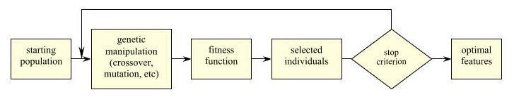
Feature selection using genetic algorithms. From [29].

3.3 State-of-the-art Classifiers

3.3.1 Neural Networks

Neural networks model a feed-forward system in which all layers except for the input layer serve as an activator that takes the outputs from the previous layer, combines them linearly, and emits its activation via a nonlinear mapping (sigmoid) function [33]. The training of a neural network is the same as fitting optimal parameters for a cost function which measures the correspondence between the actual and desired network outputs. We can define a cost function such as the classification error rate and train a neural network using various algorithms such as gradient descent back-propagation, conjugate gradient, and Newton's method [30]. Different training algorithms generate different locally optimal solutions. There have been many techniques invented to alleviate overtraining of a neural network such as momentum and learning rate [33].

3.3.2 Support Vector Machines (SVM)

Similar to neural networks, support vector machines are a set of classifiers that employ linear classifiers as building blocks. Instead of organizing linear classifiers in a network hierarchy, SVMs generalize linear classifiers using kernel functions and the maximum-margin criterion [37]. The light-weight linear classifier is often a good choice in a simple problem setting, while the linear decision boundary hypothesis is challenged in more complex problems. In addition, choosing from a group of equally good linear classifiers is sometimes error-prone. As described in KPCA, a nonlinear kernel function can be employed to transform the original feature space to a very high, sometimes unbounded, dimensional space. SVMs train linear classifiers in this very high dimensional space in that the nonlinear decision boundary can be regarded as linear after the kernel mapping. To address the difficulty of making a decision among equally behaved linear classifiers, SVMs choose the maximum-margin hyperplane as the decision boundary, which in theory minimizes the structural risk of a classifier, the upper bound on the expected test error [38]. High dimensional space is not a problem for representing the decision boundary in that only those training data points lying on the maximum-margin hyperplane, which are called support vectors, are needed.

SVMs were originally characterized for two-class problems. There have been a few methods to expand them for K-class problems [38-40]. The max-win method employs a one-vs-others strategy, in which K binary SVMs are trained to separate each class from all other classes. Given a test data point, the class with the highest output score is selected as the prediction. The pair-wise method employs a one-vs-one strategy, in which K(K-1)/2 binary SVMs are created for all possible class pairs. Each classifier gives a vote to one class given a test data point and the class with the most votes is selected as the output. Alternatively, the K(K-1)/2 binary SVMs can be put in a rooted binary DAG (Directed Acyclic Graph), where a data point is classified as not-i at each node when i is the loser class. The only class left when a leaf node is reached will be selected as the prediction. Multiclass SVMs can employ different kernel functions to differentiate protein location patterns nonlinearly.

3.3.3 AdaBoost

The training of a classifier may result in a decision boundary that performs well for a majority cluster of training data points but poorly for others. AdaBoost addresses this problem by focusing classifier training on hard examples in an iterative scheme [41]. A base classifier generator keeps generating simple classifier such as a decision tree or a one-hidden-layer neural networks. At each iteration, a simple classifier is trained with a different distribution of the entire training data with more weight associated with those points incorrectly classified from the previous iteration. By balancing the performance between correctly and incorrectly classified data, we obtain a series of classifiers, each of which remedies some errors from its predecessor while possibly introducing some new errors. The final classifier is generated by linearly combining all trained simple classifiers inversely weighted by their error rates. AdaBoost was originally characterized for two-class problems and a few expansion methods have been proposed to apply it to K-class problems [42, 43].

3.3.4 Bagging

Instead of weighting the entire training data iteratively, the Bagging approach samples the training data randomly using bootstrap replacement [44]. Each random sample contains on average 63.2% of the entire training data. A pre-selected classifier is trained repeatedly using different samples and the final classifier is an unweighted average of all trained classifiers. The motivation for bagging is the observation that many classifiers, such as neural networks and decision trees, are significantly affected by slightly skewed training data. Bagging stabilizes the selected classifier by smoothing out all possible variances and makes the expected prediction robust.

3.3.5 Mixtures-of-Experts

Similar to AdaBoost's idea of focusing a classifier on hard training examples, Mixtures-of-Experts goes one step further by training individual classifiers, also called local experts, at different data partitions and combining the results from multiple classifiers in a trainable way [45, 46]. In Mixtures-of-Experts, a gating network is employed to assign local experts to different data partitions and the local experts, which can be various classifiers, take the input data and make predictions. The gating network then combines the outputs from the local experts to form the final prediction. Both the gating network and local experts are trainable. Increasing the number of local experts in Mixtures-of-Experts will increase the complexity of the classifier in modeling the entire training data.

3.3.6 Majority-voting Classifier Ensemble

There are a large number of classifiers available in the machine learning community, each of which has its own theoretical justification. More often than not, the best performing classifier on one data set will not be the best on another data set. Given limited training data, all classifiers also suffer from overfitting. One way to alleviate the above problems is to form a classifier ensemble in which different classifiers can combine their strengths and overcome their weaknesses, assuming the error sources of their prediction are not fully correlated [44]. The most straightforward way of fusing classifiers is the simple majority-voting model. Compared to other trainable voting models, it is the fastest and performs equally well as other trainable methods [47].

In summary, the classification methods vary in the complexity of the decision boundaries they can generate, the amount of training data needed, and their sensitivity to uninformative features. Differences in their performance can therefore be expected.

3.4 Automated Interpretation of Fluorescence Microscope Images

3.4.1 Image Datasets

The goal of designing good image features and classifiers is to achieve accurate and fast automated interpretation of images. The goodness of the image features, various feature reduction methods, and classifiers must be evaluated using diverse image datasets. We therefore created several image sets in our lab and also obtained images from our colleagues. These sets contain both 2D and 3D fluorescence microscope images taken from different cell types as well as different microscopy methods. Table 3 summarizes the four image sets we used for the learning tasks described in this review.

Table 3.

Image sets used to develop and test methods for subcellular pattern analysis (Data from [50]).

Image set	Microscopy method	Objective	Pixel size in original field (microns)	No. of colors per image	No. of classes
2D CHO	Wide-field with deconvolution	100X	0.23	1	5
2D Hela	Wide-field with deconvolution	100X	0.23	2	10
3D Hela	Confocal scanning	100X	0.049	3	11
3D 3T3	Spinning disk confocal	60X	0.11	1	46

The 2D CHO dataset was collected for five location patterns in Chinese hamster ovary cells [23]. The proteins were NOP4 in the nucleus, Giantin in the Golgi complex, tubulin in the cytoskeleton, and LAMP2 in lysosomes, each of which was labeled by a specific antibody. Nuclear DNA was also labeled in parallel to each protein. The four protein classes as well as the DNA class contain different numbers of images ranging from 33 to 97. An approximate correction for out of focus fluorescence was made by nearest neighbor deconvolution using images taken 0.23 microns above and below the chosen plane of focus [48]. Since most images were taken from a field with only one cell, manual cropping was done on these images to remove any partial cells on the image boundary. The resulting images were then background subtracted using the most common nonzero pixel intensity and thresholded at a value three times higher than the background intensity. The DNA channel in this image set was not used for calculating features but for forming a fifth location class. Figure 2 shows typical images from different cells from each class of the 2D CHO dataset after preprocessing.

Figure 2.

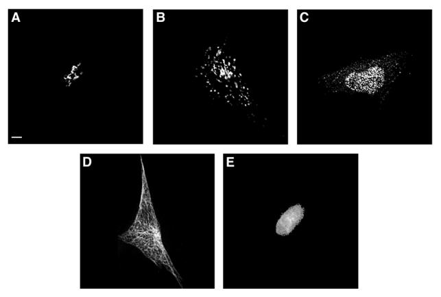
Typical images from the 5-class 2D CHO cell image collection after preprocessing. Five major subcellular location patterns are: giantin(A), LAMP2(B), NOP4(C), tubulin(D), and DNA(E). From [23].

The other collection of 2D images we have used is the 2D HeLa dataset [19]. It contains ten location patterns from nine sets of images taken from the human HeLa cell line by using the same wide-field, deconvolution approach used for the CHO set. More antibodies are available for the well-studied HeLa cell line and better 2D images can be obtained from the larger, flatter HeLa cells. This image set covers all major subcellular structures using antibodies against giantin and gpp130 in the Golgi apparatus, actin and tubulin from the cytoskeleton, a protein from the endoplasmic reticulum membrane, LAMP2 in lysosomes, transferrin receptor in endosomes, nucleolin in the nucleus, and a protein from mitochondria outer membrane [19]. The goal of including two similar proteins, Giantin and Gpp130, in this set was to test the ability of our system to distinguish similar location patterns. A secondary DNA channel was used both as an additional class and for feature calculation. Between 78 and 98 images were obtained for each class. Following the same cropping and background subtraction steps, each image was further filtered using an automatically selected threshold [49] calculated from the image. Figure 3 shows typical images from each class of the 2D HeLa dataset after preprocessing.

Figure 3.

Typical images from the 10-class 2D HeLa cell image collection after preprocessing. Each image is displayed with two false colors: red (DNA) and green (target protein).

2D images represent a single slice from the subcellular distribution of a protein, which may ignore differences in location pattern at other positions in a cell. For unpolarized cells, 2D images are usually sufficient to capture the subcellular distribution of a protein because of the flatness of the cells. For polarized cells, however, 3D images are preferred in order to describe what may be different location patterns of a protein at the “top” (apical) and “bottom” (basolateral) domains of a cell. Even for unpolarized cells, additional information may be present in a complete 3D image. We therefore collected a 3D HeLa image set using probes for the same nine proteins used the 2D HeLa set [20]. A three-laser confocal scanning microscope was used. Two parallel channels, to detect total DNA and total protein, were added for each protein resulting in a total of eleven classes, each of which had from 50 to 58 images. Each 3D image contained a stack of 14 to 24 2D slices and the resolution of each voxel was 0.049 × 0.049 × 0.2 microns (this represents oversampling relative to the Nyquist requirement by about a factor of two in each direction). The total protein channel was not only used as an additional class representing a predominantly “cytoplasmic” location pattern, it was also used for automated cell segmentation by a seeded watershed algorithm using filtering of the DNA channel to create “seeds” for each nucleus [20] (the cells on each slide are reasonably welll-separated from each other, and this seeding method was therefore observed to perform very well). Finally, background subtraction and automated thresholding were conducted on the segmented images. Figure 4 shows typical images from each class of the 3D HeLa dataset after preprocessing.

Figure 4.

Typical images from the 11-class 3D HeLa cell image collection after preprocessing. Each 3D image is displayed with three false colors: red (DNA), blue (total protein), and green (target protein). The target proteins used are the same as those of Figure 2. Two projections on the X-Y and X-Z planes are shown together.

The last image set used in our analysis was collected as part of a project to demonstrate the feasibility and utility of using CD-Tagging [13] to tag large numbers of proteins in a cultured cell line. A set of mouse NIH 3T3 cell clones expressing different GFP-tagged proteins was generated using a retroviral vector, and the identity of the tagged gene found by RT-PCR and BLAST search [16]. A number of 3D images of live cells from each clone were collected using a spinning-disk laser scanning microscope [5]. The 3D 3T3 dataset we used contained images for 46 clones, with 16 to 33 images for each clone (the size of each voxel was 0.11 × 0.11 × 0.5 microns). Each image was further processed by manual cropping to isolate single cells, background subtraction, and automatic thresholding. Figure 5 shows typical images from some of the classes in the 3D 3T3 dataset after preprocessing.

Figure 5.

Selected images from the 3D 3T3 cell image collection after preprocessing. Each image represents a major cluster from the Subcellular Location Tree created by cluster analysis [5]. Projections on the X-Y and X-Z planes are shown together.

3.4.2 Supervised Classification of Fluorescence Microscope Images

3.4.2.1 Classifying 2D Images

The first task in building our automated image interpretation system was to classify 2D fluorescence microscope images. The initial classifier we used was a neural network with one hidden layer and twenty hidden nodes. We evaluated this classifier using various feature sets and image sets. Table 4 shows the performance of this classifier for various feature sets on both 2D CHO and 2D HeLa datasets. The training of the neural network classifier was conducted on a training dataset and the training was stopped when the error of the classifier on a separate stop set no longer decreased. We evaluated the performance of the classifier using 8-fold cross validation¹ on the 2D CHO set using both the Zernike and Haralick feature sets [22, 23]. The performance using these two feature sets was similar and was much higher than a random classifier (which would have been expected to give 20% average performance on this 5-class dataset). The same classifier was then evaluated using 10-fold cross validation on the 2D HeLa set using various 2D feature sets [18, 19]. The morphological and DNA features in SLF2 gave an average accuracy of 76% on the ten location patterns. By adding both Zernike and Haralick features to SLF2 to create feature set SLF4, a 5% improvement in this performance was achieved (to 81%). Removing the six DNA features to create set SLF3 resulted in a 2% decrease, suggesting that having information on the location of the nucleus provides only a modest increase in overall ability to classify the major organelle patterns (although performance for specific classes improves more than this, data not shown).

Table 4.

Progression in classification accuracy for 2D subcellular patterns as a result of improving feature sets and optimizing classifiers.

Image dataset	Feature Set	Requires DNA image?	Number of features	Classifier	Average classifier accuracy (%)
					On test set	On training set
2D CHO	Zernike moment	no	49	NN	87	94
2D CHO	Haralick texture	no	13	NN	88	89
2D HeLa	SLF2	yes	22	NN	76	89
2D HeLa	SLF4	yes	84	NN	81	95
2D HeLa	SLF5 (SDA from SLF4)	yes	37	NN	83	95
2D HeLa	SLF3	no	78	NN	79	94
2D HeLa	SLF7	no	84	NN	74	N/A
2D HeLa	SLF8 (SDA from SLF7)	no	32	NN	86	N/A
2D HeLa	SLF13 (SDA from SLF7+DNA)	yes	31	NN	88	N/A
2D HeLa	SLF8	no	32	MV	89	N/A
2D HeLa	SLF13	yes	31	MV	91	N/A
2D HeLa	SLF15	no	44	MV	92	N/A
2D HeLa	SLF16	yes	47	MV	92	N/A

NN: one-hidden-layer neural network with 20 hidden nodes. MV: Majority voting classifier. N/A, not available.

Adding the six new features defined in SLF7 (SLF7.79-7.84), we observed a 5% decrease in accuracy compared to SLF3 alone [18]. Since all of the information present in SLF3 should be present in SLF7, the results suggested that the larger number of features interfered with the ability of the classifier to learn appropriate decision boundaries (since it required it to learn more network weights). This can be overcome by eliminating uninformative or redundant features using any of a variety of feature reduction methods. Our preliminary results for feature selection using stepwise discriminant analysis (SDA) showed anywhere from 2% improvement (SLF5 vs. SLF4) to 12% improvement (SLF8 vs. SLF7). Comparing the performances of SLF13 (which includes DNA features) and SLF8 (which does not) confirms the prior conclusion that including the DNA features provides an improvement of approximately 2%.

Since feature selection improved classification accuracy in the previous experiments, we conducted a comparison of eight different feature reduction methods (described in section 3.2) on the feature set SLF7 using the 2D HeLa image set [29]. To facilitate feature subset evaluation, a faster classifier, a multi-class support vector machine with a Gaussian kernel was used to evaluate each of the resulting feature subsets using 10-fold cross validation [29]. Table 5 shows the results of the eight feature reduction methods. Firstly, about 11% accuracy improvement was achieved by simply changing the neural network classifier to the support vector machine classifier using the same feature set SLF7. Although the four feature selection methods performed better than the four feature recombination methods in general, only the genetic algorithm and SDA gave statistically better results over SLF7 alone. Considering the minimum number of features required to achieve 80% overall accuracy, the best performance achieved after feature reduction, and the running time, SDA was the best among the eight methods. In subsequent work, we therefore used SDA as our feature selection method. SDA returns a set of features that are considered to discriminate between the classes at some specified confidence level, ranked in decreasing order of the F statistic. To determine how many of these to use for a specific classification task, we routinely train classifiers with sets of features where the ith set consists of the first i features returned by SDA and then choose the set giving the best performance.

Table 5.

Feature reduction results of eight feature reduction methods on a multi-class support vector machine with Gaussian kernel and 10-fold cross validation using the 2D HeLa image set. Feature reduction started from the feature set SLF7 which contains 84 features. (Data from [29])

Feature Selection Method	Minimum Number of Features for Over 80% Accuracy	Highest Accuracy (%)	Number of features required for highest accuracy
None	Not applicable	85.2	84
PCA	17	83.4	41
NLPCA	None found	75.3	64
KPCA	17	86.0	117
ICA	22	82.9	41
Information Gain	11	86.6	72
SDA	8	87.4	39
FDR	18	86.2	26
Genetic Algorithm	Not available	87.5	43

To further improve the classification accuracy on the 2D Hela image set, we evaluated eight different classifiers as described in section 3.3 using the feature subsets SLF13 and SLF8 (which were the best feature subsets with and without DNA features respectively). All parameters were considered changeable in these eight classifiers and the optimal ones were selected by 10-fold cross validation (Huang and Murphy, submitted). Since each classifier has its own constraints and suffers from overfitting given limited data, instead of choosing the optimal single classifier for each feature subset, we constructed an optimal majority-voting classifier ensemble by considering all possible combinations of the eight evaluated classifiers. The average performance of this majority-voting classifier was 3% higher than the neural network classifier for both SLF8 and SLF13 (Table 4).

The features used to obtain the results described so far are of a variety of types that were chosen to capture different aspects of the protein patterns. To determine whether the performance could be improved further, we explored adding a large set of new features that might duplicate those already used and employing SDA to find the best discriminative features. We therefore added 60 Gabor texture features and 30 Daubechies 4 wavelet features as described in section 3.1.1.3 to feature set SLF7 (Huang and Murphy, submitted). SDA was performed on the combined set with and without DNA features and the ranked features were evaluated incrementally by using the optimal majority-voting classifiers for SLF13 and SLF8 respectively. This resulted in two new feature sets, SLF16 which contains the best 47 features selected from the entire feature set including DNA features, and SLF15 which contains the best 44 features selected from the entire feature set excluding DNA features. The same strategy of constructing the optimal majority-voting classifier was conducted on these two new feature subsets. As seen in Table 4, the result was a small improvement in classification accuracy (to 92%) and the same accuracy was obtained with and without the DNA features (indicating that some of the new features captured approximately the same information).

The results in Table 4 summarize extensive work to optimize classification of protein patterns in 2D images, but the overall accuracy does not fully capture the ability of the systems to distinguish similar patterns. This can be displayed using a confusion matrix, which shows the percentages of images known to be in one class that are assigned by the system to each of the classes (since all of the images were acquired from coverslips for which the antibody used was known, the “ground truth” is known). Table 6 shows such a matrix for best system we have developed to date, the optimal majority-voting classifier using SLF16. Superimposed on that matrix are results for human classification of the same images [18]. These results were obtained after computer-supervised training and testing. The subject was a biologist who was well aware of cellular structure and organelle shape but without prior experience in analyzing fluorescence microscope images. The training program displayed a series of randomly chosen images from each class and informed the subject of its class. During the testing phase, the human subject was asked to classify randomly chosen unseen images from each class and the responses were recorded. The training and testing were repeated until the performance of the human subject stopped improving. The final average performance across the ten location patterns was 83%, much lower than the performance of the automated system. Except for small improvements on a couple of classes such as mitochondria and endosome, the human classifier performed worse than the automated system, especially for the two closely related classes Giantin and Gpp130. The experiment indicates that a human classifier is unable to differentiate between these two “visually indistinguishable” patterns while our methods were able to provide over 80% differentiation.

Table 6.

Classification results for the optimal majority-voting classifier on the 2D HeLa image set using feature set SLF16 compared to those for a human classifier on the same dataset. The values in each cell represent the percentage of images in the class shown on that row that are placed by the classifier in the class shown for that column (the values in parentheses are for human classification if different). The overall accuracy is 92% (vs. 83% for human classification). (Data from (Huang and Murphy, submitted) and [18].)

True Class	Output of the Classifier
	DNA	ER	Gia	Gpp	Lam	Mit	Nuc	Act	TfR	Tub
DNA	99 (100)	1   (0)	0	0	0	0	0	0	0	0
ER	0	97 (90)	0	0	0   (3)	2   (6)	0	0	0	1   (0)
Gia	0	0	91 (56)	7  (36)	0   (3)	0   (3)	0	0	2	0
Gpp	0	0	14 (53)	82 (43)	0	0	2   (0)	0	1   (3)	0
Lam	0	0	1   (6)	0	88 (73)	1   (0)	0	0	10 (20)	0
Mit	0	3	0	0	0	92 (96)	0	0	3   (0)	3   (0)
Nuc	0	0	0	0	0	0	99 (100)	0	1   (0)	0
Act	0	0	0	0	0	0	0	100 (100)	0	0
TfR	0	1  (13)	0	0	12  (3)	2	0	1   (0)	81 (83)	2  (0)
Tub	1   (0)	2   (3)	0	0	0	1   (0)	0	0   (3)	1   (0)	95 (93)

3.4.2.2 Classifying 3D Images

Given the encouraging results for classifying 2D fluorescence microscope images, we extended the evaluation to 3D fluorescence microscope images. The 3D HeLa dataset we used contains 11 subcellular location patterns, the ten patterns in the 2D HeLa dataset plus a total protein (or “cytoplasmic”) pattern. For this dataset we first evaluated the neural network classifier with one hidden layer and twenty hidden nodes using a new SLF9 feature set modeled on the morphological features of SLF2 [20]. As shown in Table 7, the average accuracy over 11 classes was 91% after 50 cross validation trials, which was close to the best 2D result. SLF9 contains morphological features derived from both the protein image and a parallel DNA images. To determine the value of the DNA features, the 14 features that require a parallel DNA image were removed from SLF9 and the remaining 14 features were defined as SLF14 (Huang and Murphy, submitted). The same neural network was trained using SLF14 on the 3D HeLa image set and the average accuracy achieved was 84%, 7% lower than for SLF9. The greater benefit from DNA features for 3D images than for 2D images could be due to at least two reasons. The first is that at least some of the non-morphological features in the larger 2D feature sets capture information that duplicates information available by reference to a DNA image, and since only morphological features were used for the 3D analysis that information was not available without the DNA features. The second is that the DNA reference provides more information in 3D space than in a 2D plane.

Table 7.

Progression in performance for 3D subcellular patterns as a result of improving feature sets and optimizing classifiers.

Image dataset	Feature Set	Requires DNA image?	Number of features	Classifier	Average classifier accuracy (%) on test set
3D HeLa	SLF9	yes	28	NN	91
	SLF14	no	14	NN	84
	SLF10 (SDA from SLF9)	yes	9	NN	94
	SLF14	no	14	MV	90
	SLF10	yes	9	MV	96

NN: one-hidden-layer neural network with 20 hidden nodes. MV: Majority voting classifier. N/A, not available.

As before, we applied stepwise discriminant analysis on SLF9 and selected the best 9 features to form the subset SLF10, for which 94% overall accuracy was achieved by employing the neural network classifier on the same image set [20]. To further improve the classification accuracy, we employed the same strategy used for 2D images by creating optimal majority-voting classifiers for both SLF10 and SLF14 (Huang and Murphy, submitted). About 6% and 2% performance improvements over the previously configured neural network classifier were observed for SLF14 and SLF10 respectively. The confusion matrix of the optimal majority-voting classifier for SLF10 on the 3D HeLa image set is shown in Table 8. Compared to the confusion matrix in Table 6, the recognition rates of most location patterns were significantly improved. The two closely related patterns, Giantin and Gpp130, now could be distinguished over 96% of the time, 14% higher than the best 2D results. It suggests that 3D fluorescence microscope images do capture more information about protein subcellular distribution than 2D images, even for unpolarized cells.

Table 8.

Confusion matrix for the optimal majority-voting classifier on the 3D HeLa image set using feature set SLF10. The overall accuracy is 96%. (Data from (Huang and Murphy, submitted))

	Cyt	DNA	ER	Gia	Gpp	Lam	Mit	Nuc	Act	TfR	Tub
Cyt	100	0	0	0	0	0	0	0	0	0	0
DNA	0	98	0	0	0	0	0	2	0	0	0
ER	0	0	97	0	0	0	0	0	2	0	2
Gia	0	0	0	98	0	2	0	0	0	0	0
Gpp	0	0	0	4	96	0	0	0	0	0	0
Lam	0	0	0	2	2	96	0	0	0	0	0
Mit	0	0	0	3	0	0	95	0	2	0	0
Nuc	0	0	0	0	0	0	0	100	0	0	0
Act	0	0	2	0	0	0	1	0	95	2	0
TfR	0	0	0	0	0	6	4	0	2	85	4
Tub	0	0	4	0	0	0	0	0	0	2	94

3.4.2.3 Implications and Cost-Performance Analysis

As discussed above, the three properties of a desirable automated image interpretation system are objectivity, accuracy, and speed. The first two properties have been demonstrated extensively above and we now turn to the computational time required for classifying images using our system. The time spent on each analysis task can be divided into three parts: image preprocessing, feature calculation, and final analysis. The preprocessing steps for both 2D and 3D images include segmentation, background subtraction, and thresholding. To calculate the cost of each feature set, we consider both the setup cost (a group of related features may share a common setup cost) and the incremental cost for each feature. Table 9 shows the times for typical classification tasks using various feature sets (Huang and Murphy, submitted). Preprocessing of 2D images needs fewer resources than the actual feature calculation. In contrast, the preprocessing step occupies the largest portion of the feature costs for 3D images. The cost of training and testing a classifier largely depends on the implementation of the specific classifier. We therefore used a support vector machine with Gaussian kernel function as an example classifier for each feature set, which performed reasonably well and was ranked as one of the top classifiers for each feature set (Huang and Murphy, 2003). Comparing all three cost components, feature calculation dominants the classification task of 2D images and image preprocessing dominates that of 3D images. Figure 6 displays the best performance of each feature set as a function of its computational cost. Using the feature set SLF13, we can expect to process about 8,000 (6 images per minute over 24 hours) 2D fluorescence microscope images per day with approximately 92% average accuracy over ten major subcellular location patterns. Of course, the calculation of many of the features we have used can potentially be speeded up dramatically by generating optimized, compiled code rather than using Matlab scripts.

Table 9.

Execution times for classifying 2D and 3D fluorescence microscope images. The number inside parentheses indicates the number of features in each feature set. Classification times shown are for training/testing of an SVM classifier. All times are for a 1.7 GHz CPU running Matlab 6.5. (Data from (Huang and Murphy, submitted))

Operation			CPU time per image (s)
Image preprocessing		2D preprocessing	0.6
		3D preprocessing	27.9
Feature calculation	2D DNA	SLF13 (31)	10.2
		SLF16 (47)	65.7
	2D	SLF8 (32)	12.6
		SLF15 (44)	67.7
	3D DNA	SLF10 (9)	4.1
	3D	SLF14 (14)	3.6
Classification	2D DNA	SLF13	1.4×10−2/5.9×10−2
		SLF16	2.1×10−2/1.1×10−1
	2D	SLF8	1.5×10−1/2.0×10−1
		SLF15	1.2×10−1/3.6×10−1
	3D DNA	SLF10	4.3×10−2/3.8×10−2
	3D	SLF14	8.5×10−2/4.8×10−2

Figure 6.

Best performance of six feature sets vs. their time costs on the 2D and 3D HeLa image collections. SLF8 (filled square), SLF10 (open diamond), SLF13 (filled diamond), SLF14 (open square), SLF15 (filled triangle), SLF16 (filled circle).

The approaches described here can be used as a roadmap for building automated systems to recognize essentially any combination of subcellular patterns in any cell type. We have described over 170 2D features and 42 3D features that can be used in combination with various feature selection and classification strategies.

3.4.2.4 Classifying Sets of Images

Cell biologists rarely draw conclusions about protein subcellular location by inspecting an image of only a single cell. Instead, a conclusion is usually drawn by examining multiple cells from one or more slides. We can improve the overall classification accuracy of automated systems in a similar manner by classifying sets of images drawn from the same class using plurality voting [19]. Theoretically, we should observe a much higher recognition rate given a classifier performing reasonably well on individual images. Two factors influence the accuracy of this approach: the number of images in each set and the number of features used for classification. Increasing the set size should enhance the accuracy such that a smaller set of features would be good enough for essentially perfect classification. On the other hand, given a larger set of good features, a smaller set size would be sufficient for accurate recognition. We have evaluated this tradeoff for the 2D and 3D HeLa datasets (Figure 7 and 8). For each feature set, random sets of a given size were drawn from the test image set for a given classifier (all images in the set were drawn from the same class) and each image was classified using the optimal majority-voting classifier for that feature set. The class receiving the most votes was assigned to that random set. This process was repeated for 1000 trials for each class.

Figure 7.

Average performance of six feature sets in image sets classification with different set sizes. SLF8 (filled square), SLF10 (open diamond), SLF13 (filled diamond), SLF14 (open square), SLF15 (filled triangle), SLF16 (filled circle).

Figure 8.

Average performance of six feature sets using different numbers of features in classifying 10-image sets. SLF8 (filled square), SLF10 (open diamond), SLF13 (filled diamond), SLF14 (open square), SLF15 (filled triangle), SLF16 (filled circle).

The results showed that the smallest image set size for an overall 99% accuracy was 7 2D images for SLF13 and 5 3D images for SLF10, respectively (Figure 7). The fewest features to achieve an average 99% accuracy given a 10-image set were the first 9 features from SLF16 on 2D images and the first 6 features from SLF10 on 3D images, respectively (Figure 8). The higher recognition rate for SLF10 on 3D HeLa images accounts for both the smaller set size and the smaller number of features required for essentially perfect classification. This approach of using an imperfect single cell classifier to achieve nearly perfect accuracy on small sets of images is anticipated to be especially useful for classifying patterns in single wells via high-throughput microscopy.

3.4.3 Unsupervised Clustering of Fluorescence Microscope Images

We have reviewed above work on supervised learning of subcellular location patterns in a number of image sets taken from different types of cells and microscopy methods. The results demonstrate not only the feasibility of training such systems for new patterns and cell types, but also demonstrate that the numerical features used are sufficient to capture the essential characteristics of protein patterns without being overly sensitive to cell size, shape and orientation. The value of these features for learning known patterns suggest that they can also be valuable for analyzing patterns for proteins whose location is unknown (or not completely known). In this section, we describe results for such unsupervised clustering of fluorescence microscope images according to their location similarity. By definition, no ground truth is available for evaluating results from unsupervised clustering, and the goodness of clustering results can only be evaluated empirically.

One of the most popular clustering algorithms is hierarchical clustering, which organizes the clusters in a tree structure. Hierarchical clustering is often conducted agglomeratively by starting with all instances as separate clusters and merging the closest two clusters at each iteration until only one cluster is left. The distance between each cluster pair can be calculated using different measures, such as the Euclidean distance and the Mahalanobis distance (which normalizes for variation within each feature and correlation between features). An average-link agglomerative hierarchical clustering algorithm was first applied for SLF8 on the 10-class 2D HeLa image set [50]. Each class was represented by the mean feature vector calculated from all images in that class. Mahalanobis distances were computed between two classes using their feature covariance matrix. The resulting tree (Subcellular Location Tree) is shown in Figure 9. This tree first groups giantin and gpp130, and then the endosome and lysosome patterns, the two most difficult pattern pairs to distinguish in supervised learning.

Figure 9.

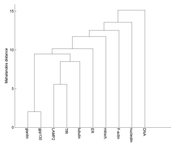
A Subcellular Location Tree (SLT) created for the 10-class 2D HeLa cell collection. From [50].

Just as protein family trees have been created that group all proteins by their sequence characteristics [51], we can also create a Subcellular Location Tree (SLT) that groups all proteins expressed in a certain cell type by their subcellular location. The data required to create comprehensive SLTs can be obtained from projects such as the CD-tagging project started a few years ago [13, 16], the goal of which was to tag all possible genes in mouse 3T3 cells and collect fluorescence microscope images of the tagged proteins. Preliminary results on clustering 3D images of the first 46 proteins to be tagged have been described [5]. The approach used is parallel to that for classification: feature selection and then selection of a clustering method.

To select the optimal features for clustering, SDA was conducted starting from feature set SLF11 (which contains 42 3D image features). For this purpose, each clone was considered to be a separate class even though some clones might show the same location pattern. The rationale was that any feature that could distinguish any two clones would be ranked highly by SDA. To decide how many of the features returned by SDA to use, a neural network classifier with one hidden layer and twenty hidden nodes was used to measure overall classification accuracy for increasing numbers of the selected features (Figure 10). The first 10 to 14 best features selected by SDA give an overall accuracy close to 70% on the 46 proteins (since some of the clones may have the same pattern, we do not expect to achieve the same high accuracy that we obtained above when the classes were known to be distinct). We therefore applied the agglomerative hierarchical clustering algorithm on the 3D 3T3 image set using the first 10 features selected from SLF11. The features were normalized to have zero mean and unit variance (z-scores) and Euclidean distances between each clone were computed from their mean feature vectors. The resulting SLT is shown in Figure 11. Evaluation of trees such as this can be difficult since if the exact location of each protein was known clustering would not be necessary. However, we can examine images from various branches from the tree to determine whether the results are at least consistent with visual interpretation. For example, two clusters of nuclear proteins can be seen in the tree: Hmga1-1, Hmga1-2, Unknown-9, Ewsh, Hmgn2-1 in one, and Unknown-11, SimilarToSiahbp1, Unknown-7 in another. By inspecting two example images selected from these two clusters as shown in Figure 12, it is obvious that the former cluster represents proteins uniquely localized in the nucleus and the latter cluster represents proteins localized in both the nucleus and the cytoplasm near the nucleus. This type of empirical comparison can heighten confidence that the tree represents an objective grouping of the location patterns.

Figure 10.

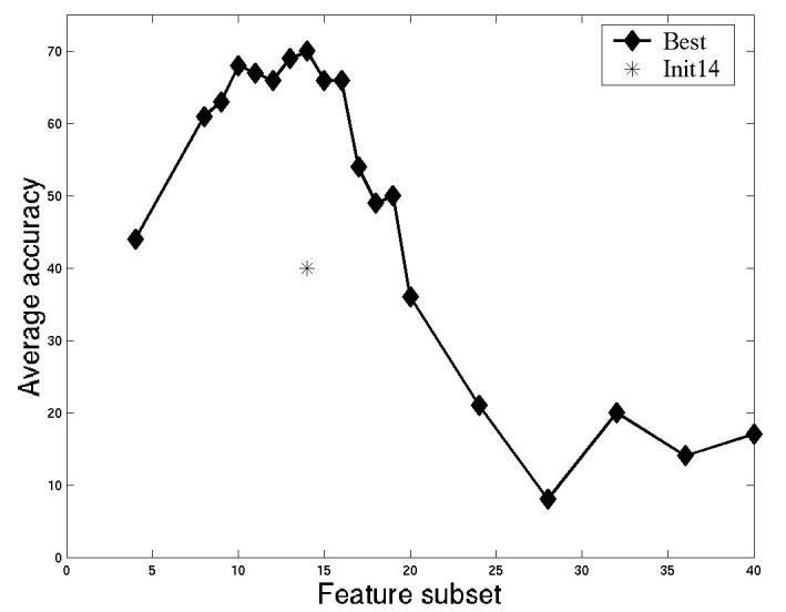
Selecting the best feature subset from SLF11 to classify the 46-class 3D 3T3 cell image collection. The average performance of a neural network classifier with one hidden layer and twenty hidden nodes after 20 cross validation trials is shown for sets comprising increasing numbers of features from SDA. From [5].

Figure 11.

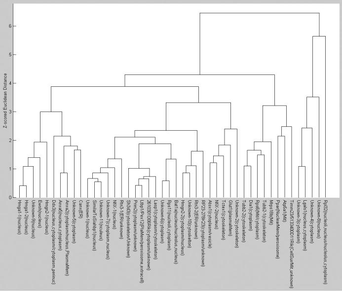
A Subcellular Location Tree created by using the best 10 features selected from SLF11 by SDA for the 46 proteins from the 3T3 image collection. From [5].

Figure 12.

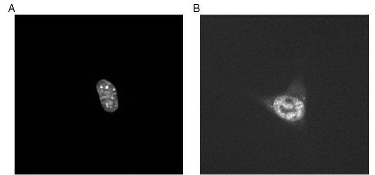
Two example images selected from the two nuclear clusters shown in Figure 11. (A) Hmga1-1; (B) Unknown-11. From [5].

3.4.4 Other Important Applications

The automated system described so far provides a validated converter that transforms the information on a protein subcellular distribution in a digital image into a set of numbers (features) that are informative enough to replace the image itself. Many off-the-shelf statistical analysis tools can be directly applied to this numerical image representation and help us to draw statistically sound conclusions for protein patterns.

3.4.4.1 Typical Image Selection

An example is to obtain the most typical image from a set of fluorescence microscope images. Typical image selection is often encountered in a situation when a very small number of images have to be selected from a large image collection. Traditionally, visual inspection is used, which is both subjective and unrepeatable given different inspectors. We have described methods that provide an objective and biologically meaningful way of ranking images by their typicality from a collection [52].

The images in a collection can be represented as a group of multidimensional data points in the feature space. The centroid of this group can be calculated by taking the mean feature vector of all data points. Distances, such as Euclidean and Mahalanobis distances, can be computed between each data point and the centroid. All images in the collection can be ranked by their distances to the centroid in the feature space and the most typical image would be the one on the top of the list [52]. To obtain the most reliable centroid, we found that outlier rejection was very helpful and provided better results than other methods. Various experiments on finding most typical images from contaminated image sets have been conducted and the results showed that the Mahalanobis distance function was better than the Euclidean distance function. Figure 13 shows results from one of the experiments. The most typical Golgi images are characterized by compact structure while the least typical ones are characterized by dispersed structure. The biological explanation for this observation is that normal Golgi complex goes through fragmentation prior to cell division and therefore a minority of cells show a dispersed pattern. The results illustrate the value of automated typicality analysis.

Figure 13.

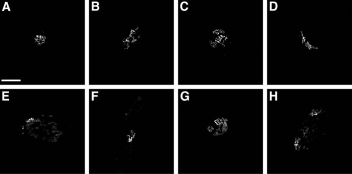
Most and least typical giantin images selected from a contaminated image set. (A-D): giantin images with high typicality; (E-H): giantin images with low typicality. From [52].

3.4.4.2 Image Set Comparison

Each fluorescence microscope image representing a certain subcellular location pattern is determined by two factors: the protein that is labeled and the environment under which the image is taken. One factor can be easily employed to infer changes of the other. For instance, the various protein subcellular location patterns can be compared to each other given a fixed environment for all classes. On the other hand, we can compare the properties of various environments (such as the presence of drugs) given a fixed protein as the reference. In both scenarios, two sets of images taken from different conditions have to be compared. We have described an objective method to compare two image sets objectively [53], which can be used in many practical applications such as drug screening and target verification.

Given our informative features, the task of comparing two image sets can be transformed to a statistical analysis that compares two feature matrices computed from the two sets. The Hotelling T²-test [54], which is the multivariate version of the t-test, can be used to compare two feature matrices. As an illustration of the approach, we performed all pairwise comparisons of the 10-class 2D HeLa set using feature set SLF6 [53]. Each comparison yielded an F value which could be compared to a critical F value for a given significance level. All pairwise F values were larger than the critical F value for 95% confidence and therefore all class pairs were considered statistically different (which is consistent with the observation that classifiers can be trained to distinguish all of them). The two pairs that gave the smallest F values were giantin with gpp130, and LAMP2 (lysosomes) with transferrin receptor (endosomes), which are again consistent with the classification and clustering results described above. To prove that the statistical test was not overly sensitive, we conducted two experiments. The first experiment was designed to compare equal-sized sets randomly drawn from the same class 1000 times. Approximately 5% of the total trials were considered to be statistically different, which is what is expected for a 95% confidence level. The second experiment was designed to compare two sets of giantin images by using different labeling approaches, a rabbit antiserum and a mouse monoclonal antibody. The resulting F value was 1.04, less than the critical F value 2.22 for 95% confidence. These two experiments confirmed that our methods were able to correctly identify two sets from the same pattern, but able to distinguish sets drawn from patterns known to be different.

As a further step, we can perform univariate t-tests to inspect the contribution of each feature to the discrimination of two image sets. Table 10 shows the features found by univariate t-tests to be most different between the giantin and gpp130 image sets. The distinction between these two sets could be largely attributable to the morphological features that describe the overall cell shape and object properties. Our objective image sets comparison method can be applied in drug screening where the candidate drug would be the one that could cause the most significant location change of a target protein. On the other hand, the optimal target could be selected as the one that displays the largest location change given a known drug.

Table 10.

Most discriminative features from SLF6 ranked by their univariate t-test results for the giantin and gpp130 image sets. (Data from [53])

Feature	Confidence level at which feature differs
Eccentricity of the ellipse equivalent to the protein image convex hull	99.99999
Convex hull roundness	99.9999
Measure edge direction homogeneity 1	99.9873
Average object size	99.9873
Average object distance to the center of fluorescence	99.9873
Ratio of largest to smallest object to image center of fluorescence distance	99.9873

4. Summary

In this review, we described an image understanding system that featured image processing, classification, clustering, and statistical analysis of fluorescence microscope images. This system is an example of applying advanced computer vision and pattern recognition techniques to digital images generated from quantitative microscopy. An objective, accurate, and high-throughput system is necessary for reliable and robust image interpretation in biomedical optics applications. Our methods, along with high-throughput imaging hardware, can be used to determine the subcellular location of every protein expressed in a certain cell type, which results in a complete location tree necessary for functional proteomics. The work described here only scratches the surface of what is possible for automated microscopy.