Spin glasses and fragile glasses: Statics, dynamics, and complexity

Abstract

In this paper I will briefly review some theoretical results that have been obtained in recent years for spin glasses and fragile glasses. I will concentrate my attention on the predictions coming from the so called broken replica symmetry approach and on their experimental verifications. I will also mention the relevance or these results for other fields, and in general for complex systems.

Spin glasses have been intensively studied in the last 30 years. They are very interesting for many reasons:

• Spin glasses are the simplest example of glassy systems. There is a highly nontrivial mean field approximation that can be used to derive some of the main properties of glassy systems, e.g., history-dependent response (1–3); this property, in the context of mean field approximation, is related to the existence of many equilibrium states. (Much ink has been used to discuss the precise mathematical meaning of this last sentence; for a careful discussion see refs. 4 and 5.)

• The study of spin glasses opens an important window for studying off-equilibrium behavior. Aging (6) and the related violations of the equilibrium fluctuation dissipation relations emerge in a natural way and they can be studied in a simple setting (7–10). Many of the ideas developed in this context can be used in other physical fields such as fragile glasses, colloids, granular materials and combinatorial optimization problems (and also for other complex systems).

• The theoretical concepts and the tools developed in the study of spin glasses are based on two logically equivalent, but very different methods: the algebraic broken replica symmetry method and the probabilistic cavity approach. They have a wide domain of applications. Some of the properties that appear in the mean field approximation, such as ultrametricity, are unexpected and counterintuitive.

• Spin glasses also provide a testing ground for a more mathematically inclined probabilistic approach: the rigorous proof of the correctness of the solution of the mean field model came out after 20 years of efforts where new ideas [e.g., stochastic stability (11–13)], and new variational principles (14, 15) were at the basis of a recent rigorous proof (16).

In this paper I will present a short review of some of the results that have been obtained by using this approach.

General Results

The simplest spin glass Hamiltonian is of the form:

where the Js are quenched (i.e., time independent) random variables located on the links connecting two points of the lattice and the σs are Ising variables (i.e., ±1). The total number of points is denoted with N and it goes to infinity in the thermodynamic limit.

We can consider four models of increasing complexity:

• The Sherrington–Kirkpatrick (SK) model (17): All Js are random and different from zero, with a Gaussian or a bimodal distribution with variance N^−1/2. The coordination number is N − 1 and it goes to infinity with N. In this case a simple mean field theory is valid in the infinite N limit (2, 3).

• The Bethe lattice model (18–20): The spins live on a random lattice and only Nz/2 Js are different from zero: they have variance z^−1/2. The average coordination number is finite (i.e., z). In this case a modified mean field theory is valid.

• The large-range Edwards–Anderson (EA) model (21): The spins belong to a finite-dimensional lattice of dimension D. Only nearest spins at a distance less than R interact and the variance of the Js is proportional to 1/R^D/2. If R is large, the corrections to mean field theory are small for thermodynamic quantities, although they may change the large-distance behavior of the correlations functions and the nature of the phase transition.

• The EA model (22): The spins belong to a finite-dimensional lattice of dimensions D: Only nearest-neighbor interactions are different from zero and their variance is D^−1/2. In this case finite corrections to mean field theory are present that are certainly very large in one or two dimensions.

As far as the free energy is concerned, one can prove the following rigorous results:

The SK model is thus a good starting point for studying also the finite-dimensional case with short-range interaction, which is the most realistic and difficult case. This starting point becomes worse and worse when the dimension decreases, e.g., it is not any more useful in the limiting case where D = 1.

Equilibrium Properties

Let us describe some of the equilibrium properties that can be computed in the mean field approximation.

At low temperature at equilibrium a large, but finite, spin glass system remains for an exponentially large time in a small region of phase space, but it may jump occasionally in a relatively short time to another region of phase space (it is like the theory of punctuated equilibria: long periods of stasis, punctuated by fast changes).

In each region α of phase space, i.e., an equilibrium state or quasi-equilibrium state, we can define a local magnetization:

When the mean field theory is valid, this magnetization satisfies the mean field equations that, neglecting the Bethe-TAP reaction-cavity term (23), can be written (in the SK limit) as

The Js are random variables. It is nontrivial to compute how many solutions this equation has and what are the properties of the solutions. The number of solutions (24) is exponential large and the precise computation of its value is a complex task (refs. 25–33; for a review, see ref. 34). The αth solution is present in the dynamics at equilibrium for a time proportional to

where f_α is the total free energy that can be computed from the magnetizations by using an explicit formula.

In general one finds that

where Σ is a nontrivial function called the complexity (35). Near the ground state the previous formula simplifies to

where f₀ = NF₀, Σ(f₀) = 0, and dΣ(x)/dx|_x=f0 ≡ y < β.

Although the number of states exponentially increases with the free energy, this increase is slower than exp(βf), and statistical sums are dominated by the lowest free energy states: a small number of states carries most of the statistical weight.

The states are macroscopically different: it is convenient to define the macroscopic distance d and the overlap q:

The states are equivalent (2): intensive observables (that depend only on a single state) have the same value in all the states, e.g., the self-overlap does not depend on the state:

Obviously, distance and overlap are related; d(α, γ)² = 2q_EA − 2q(α, γ). For historical reasons this picture is called replica symmetry breaking.

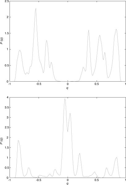
It is convenient to introduce for a given system the function P_J(q), i.e., the probability distribution of the overlap among two equilibrium configurations; see Fig. 1. Using the metaphor of having many equilibrium states, we can also write for large systems

Fig. 1.

The function P_J(q) for two samples (i.e., two choices of J) for D = 3, L = 16 (16³ spins) from ref. 36.

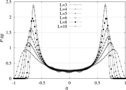
We define P(q) ≡ P_J(q), where the average is done over the different choices of the couplings J; see Fig. 2. This average is needed because the theory predicts (and numerical simulations also in three dimensions do confirm) that the function P_J(q) changes dramatically from system to system.

Fig. 2.

The function P(q) = P_J(q) after average over many samples (L = 3, …, 10) from ref. 37.

In the mean field approximation the function P(q) (and its fluctuations from system to system) can be computed analytically together with the free energy: at zero magnetic field P(q) has two delta functions at ±q_EA, with a flat part in between.

Very interesting phenomena happen when we add a very small magnetic field. The order of the states in free energy is scrambled: their free energies differ by a factor O(1) and the perturbation is of order N. Different results are obtained if we use different experimental protocols:

• If we add the field at low temperature, the system remains in the same state for a very large time, only asymptotically it jumps to one of the lower equilibrium states of the new Hamiltonian.

• If we cool the system from high temperature in a field, we likely go directly to one of the good lowest free energy states.

Correspondingly there are two susceptibilities that can be measured also experimentally:

• The so-called linear response susceptibility χ_LR, i.e., the response within a state, that is observable when we change the magnetic field at fixed temperature and we do not wait too much. This susceptibility is related to the fluctuations of the magnetization inside a given state.

• The true equilibrium susceptibility, χ_eq, which is related to the fluctuation of the magnetization when we consider also the contributions that arise from the fact that the total magnetization is slightly different (of a quantity proportional to $\sqrt{N}$) in different states. This susceptibility is very near to χ_FC, the field cooled susceptibility, where one cools the system in presence of a field.

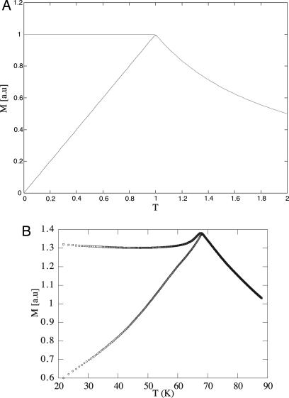
The difference of the two susceptibilities is the hallmark of replica symmetry breaking. In Fig. 3 we have both the analytic results for the SK model (2) and the experimental data on metallic spin glasses (38). The similarities among the two panels are striking.

Fig. 3.

The two susceptibilities (χ_eq ≥ χ_LR). (A) The analytic results in the mean field approximation (2). (B) The experimental results for a metallic spin glass (38).

Which are the differences of this phenomenon with a well known effect; i.e., hysteresis?

• Hysteresis is due to defects that are localized in space and produce a finite barrier in free energy. The mean life of the metastable states is finite and it is roughly exp(βΔF), where ΔF is a number of order 1 in natural units.

• In the mean field theory of spin glasses the system must cross barriers that correspond to rearrangements of arbitrary large regions of the system. The largest value of the barriers diverge in the thermodynamic limit.

• In hysteresis, if we wait enough time the two susceptibilities coincide, while they remain always different in this new framework if the applied magnetic field is small enough (nonlinear susceptibilities are divergent).

We shall see in the next section the difference between hysteresis and the new picture (replica symmetry breaking) becoming clearer as we consider fluctuation dissipation relations during aging.

Slightly Off-Equilibrium Behavior

Standard thermodynamics is very useful to understand the dynamics at equilibrium, but serious complications are present when the systems are not at equilibrium. However, some detailed results can be obtained if the system is slightly off-equilibrium. A neat theory may be formulated in the case where the time scale related to nonequilibrium phenomena is much longer than the microscopic time scales (e.g., seconds versus picoseconds). The simplest way to put a system out of equilibrium is to perturb it by changing the external parameters (temperature, magnetic field) and producing a transient behavior. In the case of a fluid we could also add a constant stirring force and produce a stationary off-equilibrium system.

The most studied case is aging. The system is cooled from a high temperature to a low temperature at time 0. In many systems the response at a time scale that is of the order of the age of the system is notably different from the equilibrium one.

When we cool the system below the critical temperature, the system has the tendency to order itself, i.e., to go to one equilibrium state. However, this process must happen locally (there is no direct long-range exchange of information), and the degrees of freedom must arrange themselves in some configurations that locally minimize the free energy. In this process we have the formation of domains where the free energy is well minimized, separated by walls with high free energy. Therefore at finite time we have the formation of a mosaic state (39–42), characterized by a dynamical length ξ(t). The function ξ(t) is an increasing function of time that eventually goes to infinity.

Whereas in the case of spinoidal decomposition there are only two equilibrium states, and the mosaic has only two colors, in the case in which there are many locally different equilibrium states, as there should be in spin glasses, each cell of the mosaic is likely to belong to a different ground state and the picture is much more complex.

In the case of the spinoidal decomposition the function ξ(t) increases relatively fast (e.g., as t^1/3). In spin glasses, the increase of the function ξ(t) is rather slow and there are indications that also in the most favorable experimental situations ξ(t) arrives to 100 (in microscopic units): the domains are rather small from the macroscopic point of view, but microscopically they may contain a large number of magnetic atoms (e.g., 10⁶). The precise form of the increase of the function ξ(t) is not very important (some authors have suggested t^α, with α of the order 0.13 in the experimentally accessible region (43, 44). An important point is that the excess of energy is proportional to a high negative power of ξ(t) [e.g., as ξ(t)⁻⁴], so that during aging energy relaxation is very small, consistent with the fact that it has never been observed experimentally, being seen only in simulations.

In this situation the system moves microscopically much more than at equilibrium, because when ξ increases different domains are rearranged and this produces an excess of thermal fluctuations. In the same way the systems may choose among different possibilities when the domains change and this may lead to an additional response to external perturbations that may influence these choices. During aging the relations between fluctuation and response are modified. The fluctuation dissipation theorem, which is at the basis of the thermodynamics and is a consequence of the so-called zeroth law of the thermodynamics, is no longer valid: a new definition of temperature is needed.

Let us show how these ideas are implemented for the aging of spin glasses. Our aim is to define a correlation function and a response function in a consistent way such that the new off-equilibrium fluctuation dissipation relations can be found.

The correlation function of total magnetization is defined as

In spin glasses at zero external magnetic field it is possible to prove that the off-diagonal terms average to zero and the only surviving term is

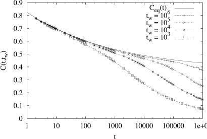
i.e., the overlap q(t_w, t_w + t) between a configuration at time t_w and one at time t_w + t (for an example taken from simulations see Fig. 4).

Fig. 4.

The correlation function for spin glasses as a function of time t at different t_w [from simulations (45)].

The relaxation function S(t, t_w) is given by

where δm is the variation of the magnetization when we add a magnetic field δh starting from time t_w.

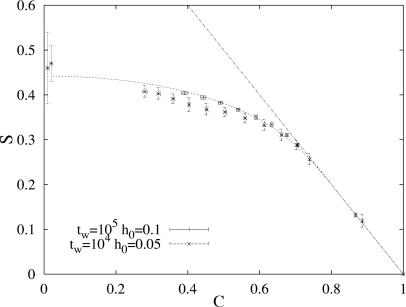
The dependence on t and t_w of the previously defined functions is rather complex and cannot be computed from general principles. It is convenient to examine directly the relation between S and C, by eliminating the time. At this end we plot parametrically S(t, t_w) versus C(t, t_w) ≡ q(t, t_w) at fixed t_w, as shown in Fig. 5.

Fig. 5.

Relaxation function versus correlation in the EA model in D = 3, T = 0.7 ≃ (¾)T_c and theoretical prediction (Ising case) (ref. 45).

The theory predicts that such a plot goes to a finite limit when t_w → ∞ and we can extract from it information on the phase structure of equilibrium configurations. Using general arguments (7, 9, 10), one finds that when t_w → ∞,

The behavior of the system at equilibrium and the modification of the fluctuation dissipation theorem off-equilibrium are strongly related. The deep reasons that are at the origin of this unexpected behavior have been discussed at length in the literature. Essentially they are based on two physical steps:

• Stochastic stability implies that the free energy distribution of the metastable states can be reconstructed from the knowledge of P(q) (10).

• The energy distribution of the metastable states is characterized by one (or more) effective temperatures (47, 48). During equilibration the extra noise comes from the jumping from one to another equilibrium state, and this explains why the value of the effective temperature enters in the off-equilibrium fluctuation dissipation relations.

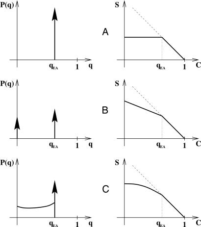
In Fig. 6 we compare the static (Left) and the dynamic (Right) behavior. On the Left we display the function P(q), and on the right, relaxation versus correlation during aging. In all the right panels the time decrease from right to left (at short times the correlation is higher). At short times, i.e., at equilibrium, the function is a straight line (with slope −1), according to the fluctuation dissipation theorem. The interesting part is the one at left, where at large times, in the aging regime, the curve deviates from the previous straight line. The value of the relaxation at the point where the equilibrium regime ends is the linear response susceptibility χ_LR, whereas the value of the relaxation on the left-most point is the equilibrium susceptibility χ_eq. We have essentially three different situations summarized in Fig. 6:

• A: Old-fashioned hysteresis. During aging there is an excess of noise with respect to equilibrium, as an effect of the microscopic movements, but these movements do not affect the response function. The presence of noise without a corresponding response is typical of a system at infinite temperature. Indeed, the effective temperature βX(C) is infinite in the aging region.

• B: A new and nontrivial phenomenon, that should be present in structural fragile glasses and in some kinds of spin glasses. The system has two temperatures, and both are finite (47–50). Often the higher temperature is near to the critical temperature.

• C: A more complex phenomenon that is present in the mean field theory of some spin glasses (e.g., in the original SK model). It corresponds to the presence of a continuous range of temperatures in the aging region.

Fig. 6.

Three different forms (A, B, and C) of the function P(q) (Left) and the related function S(q) (Right). Delta functions are represented as a vertical arrow (taken from ref. 46).

The presence of anomalies in the off-equilibrium regime in the plot of the response versus correlations (i.e., cases B and C) marks in a clear way the difference from the old picture (hysteresis). The experimental fact that in real spin glasses χ_LR ≠ χ_eq excludes case A.

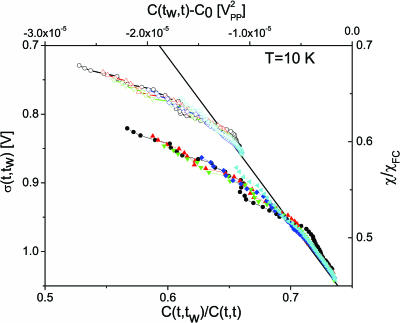
In the case of Ising spin glasses with two body interaction in the mean field approximation we stay in case C. What happens in three dimensions is not clear. Numerical simulations (5, 36, 37, 45) on Ising model indicates that we stay in case C, whereas the experiments (51) (shown in Fig. 7) show a clear effect of deviations from case A that may indicate more case B. From the theoretical viewpoint there are no firm commitments: although in infinite dimensions with a two-spin interaction we are in case C, the corrections due to the interaction among the fluctuations could bring the system in three dimensions in case B.

Fig. 7.

Experimental raw results (filled symbols) and ageing part (open symbols) deduced from the scaling analysis. The different curves span the waiting times studied: t_w = 100 s, t_w = 200 s, t_w = 500 s, t_w = 1000 s, t_w = 2000 s (from ref. 51).

This difference between the simulations and the experiment may have two different origins:

• The experiment and the numerical simulations do correspond to two different regimes: the time scales are quite different. Moreover, if experimentally we cool a high-temperature system, thermalized domains grow with time and the maximum experimental reachable side is about 100. In simulations a compact system can be thermalized up to size 20.

• The numerical simulations are mostly done on Ising systems, whereas the experiments have been mostly done on more Heisenberg systems with anisotropy and a long-range tail of interactions (other systems are more complex); there are indications from other properties that the two systems behave in a different manner.

More extended numerical simulations and experimental results on other systems are needed to decide which picture is correct. One should also consider the possibility that the correlation length in the equilibrium limit remains fine, but very large (e.g., 1,000 lattice units). In such a case one should see the effects of broken replica symmetries for times of human scale and only for astronomical times should the anomaly disappear. The possibility of this phenomenon is difficult to dismiss, but it would not jeopardize the interpretation of the experimental data using spontaneously broken replica theory.

Structural fragile glasses will be discussed later. Here we notice that numerical simulations and strong theoretical arguments point to the fact that they should belong to case B. Unfortunately, although deviations from the equilibrium fluctuation dissipation relations have been observed in structural glasses, the situation is not so clear as for spin glasses.

Other impressive phenomena that happen mainly in spin glass are memory and rejuvenation (52). Unfortunately I cannot discuss them for lack of space.

Structural Fragile Glasses

Some of the physical ideas that have been developed for spin glasses have also been developed independently by people working in the study of structural glasses. However, in the fields of structural glasses there were no soluble models that displayed interesting behavior, so most of the analytic tools and of the corresponding physical insight were first developed for spin glasses.

The two fields remained quite separate from one another also because there was a widespread belief that the presence of quenched disorder (absent in structural glasses) was a crucial ingredient of the theory developed for spin glasses. Only in the middle of the 1990s did it become clear that this was a misconception (53, 54) and it was realized that the spin glass theory may be applied also to systems where nonintrinsic disorder is present (e.g., hard spheres).

This became manifest after the discovery of models where there is a transition from a high-temperature liquid phase to a low-temperature glassy phase (some of these models at low temperature have two phases, a disorder phase and an ordered, crystal phase). Spin glass theory was able to predict the correct behavior both at high and at low temperature.

The simplest model is the so-called sin model (53), which differs form the SK in the choice of the coupling by having

The crystal state apparently exists only for some values of N: e.g., for N prime of the form 4k + 1, where the ground state is given by σ_i ≡_{mod N i^2k}. It is an interesting and unsolved mathematical problem (55) to find all the values of N where crystal states exist; however, this is not relevant for the behavior of the system in the glassy phase, where the system is cooled fast enough to avoid crystallization.

This discovery led to a better understanding of the replica method that was applied also to study the properties of fragile glasses. By using this method it was possible to solve a large number of models where some of the ideas and tools (e.g., configurational entropy, entropy crisis, mode coupling equations) can be treated in an explicit and unified way (56). The method also allows analytic computations of properties of glasses at low temperature for hard and soft spheres, where the whole low-temperature phase diagram can be obtained by using simple integral equations such as generalized hypernetted chain (HNC) equations (57–61).

One finds, in agreement with experiments, that there is a dynamical phase transition (more precisely a crossover point) below which the relaxation becomes very slow (on a microscopic scale) and it is dominated by tunnel events: this is the so-called mode-coupling transition (56, 62). The physical interpretation of this transition is rather simple: above the phase transition the system is near a saddle point of the Hamiltonian, whereas below it the system is near a local minimum of the Hamiltonian (63–67). This picture is very interesting, also because it gives a clear explanation of the origin and of the properties of the celebrated boson peak (68). There is also a true phase transition where the relaxation time becomes infinitely large [it diverges as exp(A/(T − T_K)^α)] where the specific heat is discontinuous.

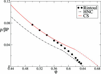
Just as an example we show in Fig. 8 the result of recent analytic computation of the inverse of the pressure for a (noncrystallizing) liquid of hard spheres, where one finds a maximal amorphous packing of φ ≈ 0.64 (if we use a better approximation we find a similar value, i.e., φ ≈ 0.68).

Fig. 8.

Inverse of the reduced pressure of the hard sphere liquid as a function of packing fraction φ (69). The filled circles are from the simulation of Rintoul and Torquato (70). The dot–dashed line is obtained by using the HNC equation of state, and the orange line is obtained by using the Carnahan–Sterling equation of state (70).

Other Applications

There are many problems for which these ideas have been used. In the past there has been a great interest in applying them to problems with a biological flavor, like the computation of the optimal performance of associative memories based on neural networks (see, for example, ref. 71). In addition, learning abilities of simpler objects such as the perceptrons can be computed.

In recent years these ideas have been widely used in the field of combinatorial optimization problems and constraint satisfaction. The first example of optimization problems that has been studied with these techniques is the random assignment problem. We have N cities and N wells; the distance among the cities and the wells is an N × N matrix whose entries are random numbers with a flat distribution in the interval [0–1]. We want to assign each city to each well in such way to minimize the total distance. In these case one can show that the average length of the optimal assignment is given by (72, 73)

The correctness of the leading term has been proved by mathematicians in a remarkable paper (74). The leading term does not depend on the instance, while the subleading term depends on the instances and the value quoted is the average of the different instances, and a rigorous proof of its correctness is missing.

More recently, random satisfaction models were intensively studied, also because the techniques developed in refs. (75 and 76) for studying spin glasses on Bethe lattices allowed us to tackle these models. The simplest example of a nontrivial random satisfaction model is coloring of a graph. We consider the ensemble of all the graphs with N nodes and M edges. We would like to find out (with probability 1) when N goes to infinity, keeping fixed the ratio M/N ≡ α, if a generic graph of this ensemble can be colored with q colors with the constraint that nodes that are connected by an edge have a different color.

For each given value of q there is a critical value of α, i.e., α_c(q) such that for α < α_c(q) the graph can be colored with q colors, whereas for α > α_c(q) the graph cannot be colored. From the physical point of view this model is an antiferromagnetic Potts model with q states (the energy has a positive nonzero contribution if two spins connected by an edge are in same state) and we are asking if the ground state energy density is zero or nonzero. The computation (although a rigorous proof is lacking) of α_c(q) has been obtained in recent times (77): for example, one finds α_c(3) = 4.69 and α_c(4) = 8.90.

The techniques used were introduced to study spin glasses on the Bethe lattice and have been applied to the study of the transition from satisfiability to unsatisfiability in the case of K-satisfiability (from the physical point of view an Ising spin system with a peculiar K-body quenched interaction). In the case of the celebrated 3-Sat problem (78) it was found that α_c = 4.267. Similar ideas have been applied to error correcting codes starting from the seminal work of Sourlas (79).

Complex Systems: A Surprise

Spin glasses have many interesting properties (at least in the mean field approximation) that were completely unexpected.

We have already remarked that a given finite but very large system has many equilibrium states; a schematic description of these states is the set of all the values of the weights ws and of the overlaps qs. Let us denote it by 𝒟_J = {w_α, q_α,γ}. In usual systems the set is nontrivial only at a first-order phase transition point and we have to tune K parameters to have the coexistence of K + 1 states (Gibbs rule). In spin glasses there is a large number of equilibrium states in variance with the Gibbs rule: spin glasses can be thought to stay always at a critical point and they can be considered as an equilibrium version of self-organized criticality (78).

Moreover, the number of equilibrium states is diverging when the volume goes to infinity: of course most of the states carry a very small weight (i.e., they are high free energy states). In the infinite volume limit the number of states that carry a weight higher than ε diverges as

where y is a number that depends on the parameter of the system.

In some sense the system is unstable. If we change a large but finite number of the coupling Js, the free energies of the states change by an amount that is much bigger than the distance among levels and the states that have higher weight are different: ground state becomes metastable states (the same phenomenon is present if we change global parameters of the systems such as the magnetic field (78). The function P_J(q) also becomes quite different after a perturbation. The schematic description of the states system 𝒟_J, which we have previously introduced, has a chaotic dependence on the parameters of the systems and for all practical purposes is incomputable (for a large system). For given N, if we average over the J, we have a probability distribution of the descriptors 𝒫(𝒟). The function P(q) [i.e., the average over an ensemble of systems of the various P_J(q) functions] can be reconstructed from the knowledge of the functional 𝒫(𝒟) (I use the word functional because 𝒟 belongs to an infinite-dimensional space). Although the structure of the lowest free energy states depend on the system, this dependence becomes weaker when we consider higher free energy states.

This instability is balanced by the property of stochastic stability that asserts that the distribution 𝒫(𝒟) is stable with respect to perturbations (11–13). This property has far-reaching consequences (it is far from being trivial, because the individual weights ws change of a large amount under a perturbation). For example, stochastic stability implies that it is possible, by analyzing the properties of a single large system, to reconstruct the properties of the whole 𝒫(𝒟) averaged over the ensemble of systems to which the individual system naturally belong (49, 50): in a similar way the fluctuation dissipation relations tell us that we can reconstruct the P(q) function from the analysis of the response and the correlations during aging.

The last surprise was ultrametricity. If we use the distance defined in Eq. 9 the following inequality holds (2):

Under the previous conditions, P(q) = Σ_α,γ w_αwγδ(q_α,γ−q) determines analytically the full 𝒫(𝒟) (ref. 80).

The inequality 18 implies that the most relevant states form an ultrametric tree, i.e. they can be put on a tree in such a way that the states are on the branches of the tree and the distance among the states is the maximum level one has to cross for going from one state to another. In other words the states of a system can be classified in a taxonomic way. The most studied possibilities are the following:

• All different states are at given distance d from one another and the taxonomy is rather trivial (one-step replica symmetry breaking: case B).

• The states have a continuous distribution and branching points exist at any level (continuous replica symmetry breaking: case C). A suggestive drawing of how the tree may look, if we draw only the finite number of branches that have weight larger than ε, is shown in Fig. 9. A careful analysis of the properties of the tree can be found in refs. 81 and 82.

Fig. 9.

An example of a taxonomic tree of states in the case of a hierarchical breaking of the replica symmetry.

Other distributions are possible, but they are less common or at least less studied.

It is remarkable that, if ultrametricity and stochastic stability are true, the function P(q) completely determines the functional 𝒫(𝒟). Moreover, in the SK model, the functional 𝒫(𝒟) determines the value of the equilibrium free energy: one can define a free energy functional ℱ[𝒫] such that

In the case of an ultrametric and stochastic stable 𝒫(𝒟), using an auxiliary differential equation, we can write an explicit expression for a free energy functional ℱ[𝒫], and in this way it is possible to find the value of the free energy with accurate precision. It has been mathematically proved that the ultrametric functional 𝒫(𝒟) gives the correct maximum (16). We miss only the information about the unicity (or not) of the maximum.

Summarizing, the system may stay in an infinite number of different equilibrium states, and an appropriate perturbation forces the system to switch from one state to another one. The precise form of the lower-lying states has a chaotic dependence on the space of parameters and it is practically incomputable for large systems (these states physically are never reached because the time would be too long). The different equilibrium states have a hierarchical structure that leads to a taxonomic classification of the states.

All these feature are typical of what is called a complex system (83, 84): the existence of many states, the practical impossibility of finding the most stable state among all the metastable states and the hierarchical structure of states are features that spin glasses share with many other natural complex system, so that spin glasses are the prototype of complex systems. Many ideas that have been developed in this context by physicists have a much wider range of applications to natural complex systems that are present in other sciences. The study of complex systems is now a fascinating growing discipline.

Conclusions

From the retrospective point of view, the amount of new ideas that have been necessary to understand in depth the basic properties of spin glasses and other glassy systems seems extraordinary. A strong effort should be made to have better quantitative predictions and a more precise comparison between theory and experiments. There are open problems where I would like to see a progress:

• A systematic and careful experimental study of the fluctuation–dissipation relations is needed to extend our knowledge on this very interesting and fundamental phenomenon.

• It would be important to obtain more precise understanding of the glass transition in structural fragile glass; in particular, it would be very useful to get quantitative predictions on the behavior of the dynamics in the region where it is dominated by escapes from barriers.

• New results should be obtained of the form of time behavior in nonequilibrium state, where only partial results are known.

• To arrive at a precise assessment of the behavior of three-dimensional spin glasses it would be very important to develop further the renormalization group approach and/or other theoretical or experimental techniques.

• It also may be worthwhile to study again some of the problems on automatic machine learning, as the comparison among different architecture (85), that were started 20 years ago, but never arrived at a clear analytic conclusion.

• Last, but not least, I would like to see a clear discussion of the relevance of the approach to the behavior of glasses in the low temperature phase region, where quantum phenomena dominate the scene.

It is also possible that the most exciting result will come from an area I am not able to indicate. I am very curious to see the future of the field.

Abbreviations

EA

Edwards–Anderson

SK

Sherrington–Kirkpatrick.

References

- 1.Anderson P. W. In: Ill-Condensed Matter. Balian R., Maynard R., Toulouse G., editors. North-Holland, Berlin: 1983. pp. 159–259. [Google Scholar]
- 2.Mézard M., Parisi G., Virasoro M. A. Spin Glass Theory and Beyond. Singapore: World Scientific; 1987. [Google Scholar]
- 3.Parisi G. Field Theory, Disorder and Simulations. Singapore: World Scientific; 1992. [Google Scholar]
- 4.Newman C. M., Stein D. L. J. Stat. Phys. 1996;82:1113–1132. [Google Scholar]
- 5.Marinari E., Parisi G., Ricci-Tersenghi F., Ruiz-Lorenzo J., Zuliani F. J. Stat. Phys. 2000;98:973–1074. [Google Scholar]
- 6.Bouchaud J.-P. J. Phys. France. 1992;2:1705–1713. [Google Scholar]
- 7.Cugliandolo L. F., Kurchan J. Phys. Rev. Lett. 1993;71:173–176. doi: 10.1103/PhysRevLett.71.173. [DOI] [PubMed] [Google Scholar]
- 8.Cugliandolo L. F., Kurchan J. J. Phys. A Math. 1994;27:5749–5771. [Google Scholar]
- 9.Franz S., Mézard M. Europhys. Lett. 1994;26:209–214. [Google Scholar]
- 10.Franz S., Mézard M., Parisi G., Peliti L. J. Stat. Phys. 1999;97:459–473. [Google Scholar]
- 11.Guerra F. Int. J. Phys. B. 1997;10:1675–1675. [Google Scholar]
- 12.Aizenman M., Contucci P. J. Stat. Phys. 1998;92:765–783. [Google Scholar]
- 13.Parisi G. 1998 cond-mat/980108. [Google Scholar]
- 14.Guerra F. Comm. Math. Phys. 2002;233:1–12. [Google Scholar]
- 15.Aizenman M., Sims R., Starr S. L. Phys. Rev. B. 2003;68:214403. [Google Scholar]
- 16.Talagrand M. Ann. Math. 2006;163:221–263. [Google Scholar]
- 17.Sherrington D., Kirkpatrick S. Phys. Rev. Lett. 1975;35:1792–1796. [Google Scholar]
- 18.Viana L., Bray A. J. J. Phys. C. 1985;18:3037–3051. [Google Scholar]
- 19.Mézard M., Parisi G. Eur. Phys. J. B. 2001;20:217–233. [Google Scholar]
- 20.Mézard M., Parisi G. J. Stat. Phys. 2003;111:1–23. [Google Scholar]
- 21.Franz S., Leone M. J. Stat. Phys. 2003;111:535–564. [Google Scholar]
- 22.Edwards S., Anderson P. J. J. Phys. F. 1975;5:965–979. [Google Scholar]
- 23.Thouless D. J., Anderson P. A., Palmer R. G. Phil. Mag. 1977;35:593–607. [Google Scholar]
- 24.Bray A. J., Moore M. A. J. Phys. A. 1980;13:L469–L476. [Google Scholar]
- 25.Cavagna A., Giardina I., Parisi G., Mézard M. J. Phys. A. 2003;36:1175–1197. [Google Scholar]
- 26.Aspelmeier T., Bray A. J., Moore M. A. Phys. Rev. Lett. 2004;92:087203. doi: 10.1103/PhysRevLett.92.087203. [DOI] [PubMed] [Google Scholar]
- 27.Crisanti A., Leuzzi L., Parisi G., Rizzo T. Phys. Rev. B. 2003;68:174401. doi: 10.1103/PhysRevLett.92.127203. [DOI] [PubMed] [Google Scholar]
- 28.Cavagna A., Giardina I., Parisi G. J. Phys. A. 1997;30:7021–7038. [Google Scholar]
- 29.Cavagna A., Giardina I., Parisi G. Phys. Rev. Lett. 2004;92:120603. doi: 10.1103/PhysRevLett.92.120603. [DOI] [PubMed] [Google Scholar]
- 30.Cavagna A., Giardina I., Parisi G. Phys. Rev. B. 2005;71:024422. [Google Scholar]
- 31.Annibale A., Cavagna A., Giardina I., Parisi G. Phys. Rev. E. 2003;68:061103. doi: 10.1103/PhysRevE.68.061103. [DOI] [PubMed] [Google Scholar]
- 32.Crisanti A., Rizzo T. Phys. Rev. E. 2002;65:046137. doi: 10.1103/PhysRevE.65.046137. [DOI] [PubMed] [Google Scholar]
- 33.Rizzo T. J. Phys. A. 2005;38:3287–3297. [Google Scholar]
- 34.Parisi G. Proceedings of the Les Houches Summer School 2005; Amsterdam: Elsevier; 2006. in press. [Google Scholar]
- 35.Monasson R. Phys. Rev. Lett. 1995;75:2847–2850. doi: 10.1103/PhysRevLett.75.2847. [DOI] [PubMed] [Google Scholar]
- 36.Marinari E., Parisi G., Ruiz-Lorenzo J. J. In: Spin Glasses and Random Fields. Young P., editor. Singapore: World Scientific; 1998. pp. 58–98. [Google Scholar]
- 37.Marinari E., Zuliani F. J. Phys. A. 1999;32:7447–7461. [Google Scholar]
- 38.Djurberg C., Jonason K., Nordblad P. Eur. Phys. J. B. 1998;10:15. [Google Scholar]
- 39.Kirkpatrick T. R., Wolynes P. G. Phys. Rev. B. 1987;36:8552–8564. doi: 10.1103/physrevb.36.8552. [DOI] [PubMed] [Google Scholar]
- 40.Kirkpatrick T. R., Thirumalai D. Transp. Theor. Stat. Phys. 1995;24:927. [Google Scholar]
- 41.Franz S., Parisi G. J. Phys. C. 2000;12:6335–6349. [Google Scholar]
- 42.Bouchaud J.-P., Biroli G. Phys. Rev. B. 2005;72:064204. [Google Scholar]
- 43.Marinari E., Parisi G., Ruiz-Lorenzo J., Ritort F. Phys. Rev. Lett. 1996;76:843–846. doi: 10.1103/PhysRevLett.76.843. [DOI] [PubMed] [Google Scholar]
- 44.Joh Y. G., Orbach R., Wood G. G., Hammann J., Vincent E. Phys. Rev. Lett. 1999;82:438–441. [Google Scholar]
- 45.Marinari E., Parisi G., Ricci-Tersenghi F., Ruiz-Lorenzo J. J. J. Phys. A. 1998;31:2611–2620. [Google Scholar]
- 46.Parisi G., Ricci-Tersenghi F., Ruiz-Lorenzo J. J. Eur. Phys. J. B. 1999;11:317–325. [Google Scholar]
- 47.Cugliandolo L., Kurchan J., Peliti L. Phys. Rev. E. 1997;55:3898–3814. [Google Scholar]
- 48.Franz S., Virasoro M. A. J. Phys. A. 2000;33:891–905. [Google Scholar]
- 49.Parisi G. J. Phys. A. 2003;36:10773–10789. [Google Scholar]
- 50.Parisi G. Europhys. Lett. 2004;65:103–109. [Google Scholar]
- 51.Herisson D., Ocio M. Phys. Rev. Lett. 2002;88:257202. doi: 10.1103/PhysRevLett.88.257202. [DOI] [PubMed] [Google Scholar]
- 52.Jonason K., Vincent E., Hammann J., Bouchaud J. P., Nordblad P. Phys. Rev. Lett. 1998;81:3243–3246. [Google Scholar]
- 53.Marinari E., Parisi G., Ritort F. J. Phys. A. 1994;27:7647. [Google Scholar]
- 54.Bouchaud J.-P., Mézard M. J. Physique. 1994;4:1109–1120. [Google Scholar]
- 55.Degli Esposti M., Giardinà C., Graffi S., Isola S. J. Stat. Phys. 2001;102:1285–1313. [Google Scholar]
- 56.Bouchaud J.-P., Cugliandolo L., Kurchan J., Mézard M. Physica A. 1996;226:243–276. [Google Scholar]
- 57.Mézard M., Parisi G. J. Phys. A. 1996;29:651–672. [Google Scholar]
- 58.Mézard M., Parisi G. Phys. Rev. Lett. 1999;82:747–750. [Google Scholar]
- 59.Coluzzi B., Mézard M., Parisi G., Verrocchio P. J. Chem. Phys. 1999;111:1076–1093. [Google Scholar]
- 60.Coluzzi B., Parisi G., Verrocchio P. J. Chem. Phys. 2000;112:2933–2949. doi: 10.1103/PhysRevLett.84.306. [DOI] [PubMed] [Google Scholar]
- 61.Coluzzi B., Parisi G., Verrocchio P. Phys. Rev. Lett. 2000;84:306–309. doi: 10.1103/PhysRevLett.84.306. [DOI] [PubMed] [Google Scholar]
- 62.Götze W., Sjogren L. J. Phys. C. 1992;21:3407–3421. [Google Scholar]
- 63.Cavagna A. Europhys. Lett. 2001;53:490–496. [Google Scholar]
- 64.Angelani L., Di Leonardo R., Ruocco G., Scala A., Sciortino F. . Phys. Rev. Lett. 2000;85:5356–5339. doi: 10.1103/PhysRevLett.85.5356. [DOI] [PubMed] [Google Scholar]
- 65.Broderix K., Bhattacharya K. K., Cavagna A., Zippelius A., Giardina I. Phys. Rev. Lett. 2000;85:5360–5363. doi: 10.1103/PhysRevLett.85.5360. [DOI] [PubMed] [Google Scholar]
- 66.Grigera T. S., Cavagna A., Giardina I., Parisi G. Phys. Rev. Lett. 2002;88:055502. doi: 10.1103/PhysRevLett.88.055502. [DOI] [PubMed] [Google Scholar]
- 67.Cavagna A., Giardina I., Parisi G. Phys. Rev. Lett. 1999;83:108–111. [Google Scholar]
- 68.Grigera T. S., Martín-Mayor V., Parisi G., Verrocchio P. Phys. Rev. Lett. 2001;87:085502. doi: 10.1103/PhysRevLett.87.085502. [DOI] [PubMed] [Google Scholar]
- 69.Parisi G., Zamponi F. J. Chem. Phys. 2005;123:144501. doi: 10.1063/1.2041507. [DOI] [PubMed] [Google Scholar]
- 70.Rintoul M., Torquato S. Phys. Rev. Lett. 1996;77:41984201. doi: 10.1103/PhysRevLett.77.4198. [DOI] [PubMed] [Google Scholar]
- 71.Amit D. J. Modeling Brain Functions. Cambridge, U.K.: Cambridge Univ. Press; 1989. [Google Scholar]
- 72.Mézard M., Parisi G. Eur. Phys. Lett. 1986;2:913–919. [Google Scholar]
- 73.Parisi G., Ratiéville M. Eur. Phys. J. B. 2002;29:457–468. [Google Scholar]
- 74.Aldous D. Random Struct. Alg. 2001;18:381–418. [Google Scholar]
- 75.Mézard M., Parisi G. Eur. Phys. J. B. 2001;20:217–239. [Google Scholar]
- 76.Mézard M., Parisi G. J. Stat. Phys. 2003;111:1–23. [Google Scholar]
- 77.Mulet R., Pagnani A., Weigt M., Zecchina R. Phys. Rev. Lett. 2002;89:268701. doi: 10.1103/PhysRevLett.89.268701. [DOI] [PubMed] [Google Scholar]
- 78.Mézard M., Parisi G., Zecchina R. Science. 2002;297:812–816. doi: 10.1126/science.1073287. [DOI] [PubMed] [Google Scholar]
- 79.Sourlas N. Nature. 1989;339:693–696. [Google Scholar]
- 80.Iniguez D., Parisi G., Ruiz-Lorenzo J. J. J. Phys. A. 1996;29:4337–4353. [Google Scholar]
- 81.Ruelle D. Commun. Math. Phys. 1988;48:351–366. [Google Scholar]
- 82.Parisi G. J. Stat. Phys. 1993;72:857–872. [Google Scholar]
- 83.Parisi G. Physica Scripta. 1987;35:123–125. [Google Scholar]
- 84.Parisi G. In: Perspectives on Biological Complexity. Solbrig O. T., Nicolis G., editors. Paris: Int. Union Biol. Sci.; 1994. pp. 87–121. [Google Scholar]
- 85.Parisi G., Slanina F. Europhys. Lett. 1992;17:497–504. [Google Scholar]