Autoshaped Head Poking in the Mouse: A Quantitative Analysis of the Learning Curve

Abstract

In autoshaping experiments, we quantified the acquisition of anticipatory head poking in individual mice, using an algorithm that finds changes in the slope of a cumulative record. In most mice, upward changes in the amount of anticipatory poking per trial were abrupt, and tended to occur at session boundaries, suggesting that the session is as significant a unit of experience as the trial. There were large individual differences in the latency to the onset of vigorous responding. “Asymptotic” performance was unstable; large, bidirectional, and relatively enduring changes were common. Given the characteristics of the individual learning curves, it is unlikely that physiologically meaningful estimates of rate of learning can be extracted from group-average learning curves.

Behavioral neuroscientists use conditioning paradigms to evaluate the effects of brain manipulations on learning and memory. In these paradigms, the progress of learning is indicated by an increase in the rate or magnitude of the conditioned response as a function of the number of trials. Underlying this approach is the assumption that, on each trial, there is an increment in the underlying associations, whose strengths determine the observed vigor of responding.

The most common models of the underlying process of association formation (e.g., Mackintosh, 1975; Pearce & Hall, 1980; Rescorla & Wagner, 1972) assume that the process obeys first-order kinetics, in which case associative strength is an inverse exponential function of the number of trials. That is, an equation of the form 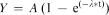is assumed to describe the process, where A and λ are the parameters of asymptote and rate, respectively.

The assumption that learning involves a gradual strengthening of underlying connections, which is reflected in the gradually increasing strength of behavior, accounts, at least approximately, for the commonly observed form of the group-average learning curve, which is a plot of the strength or rate of conditioned responses as a function of experimental trials, averaged across blocks of trials within subjects and subsequently across subjects (see, for example, Rescorla, 2002). The congruence between group-average data and the commonly accepted theoretical conceptions about what is occurring in the brains of individual subjects has led neurobiologically oriented researchers to use group-average curves to compare rates of learning between groups of subjects given different treatments, such as brain lesions (Kim & Fanselow, 1992; Morris, Garrud, Rawlins, & O'Keefe, 1982), administration of pharmacological substances (Morris, Anderson, Lynch, & Baudry, 1986), and more recently gene targeting (Sakimura et al., 1995; Shibuki et al., 1996; Silva, Paylor, Wehner, & Tonegawa, 1992; Tsien, Huerta, & Tonegawa, 1996) or transgenics (Bach, Hawkins, Osman, Kandel, & Mayford, 1995; Kishimoto et al., 2002; Lu et al., 1997; Tang et al., 1999). From these comparisons, conclusions are drawn about the effects of the neurobiological manipulations on the rate of learning.

However, it has often been pointed out that the group-average learning curve may not describe what is seen in individual subjects (Brown & Heathcote, 2003; Estes, 1956; Krechevsky, 1932; Lashley, 1942; Mazur & Hastie, 1978; Restle, 1965). If the change in the strength of each individual subject's behavior is step-like, but the steps occur after different amounts of experience and have different heights, averaging across them yields a gradually asymptoting function, the parameters of which do not estimate the values of the parameters of any function appropriate to an individual subject.

Despite the frequently expressed reservations about the validity of group-average learning curves, there has not been until recently (Gallistel, Fairhurst, & Balsam, 2004) a systematic effort to determine the course of the behavioral change in the individual subject. This is particularly important in the case of the mouse because it is so often the species used in contemporary between-group comparisons of learning rates. The object of the experiment reported here is to characterize the learning curve in individual mice in an appetitive-learning paradigm: autoshaped head poking (hopper conditioning) in the mouse.

In pilot work, we observed that the biggest changes in the level of conditioned responding often occurred between the end of one session and the start of the next. In other words, the session appeared to be an important unit of experience. It is well established that spacing trials increases rate of learning (that is, it reduces trials to acquisition)—for a review, see Barela (1999). Thus, we decided to manipulate session spacing to see whether this, too, leads to faster acquisition.

In all our experiments, we allowed the mice to self-initiate trials. We did this because we were interested in the timing of the first response (first poke latency). Our procedure fixed the mouse's position at the start of each trial, and it ensured that no poke was in progress when a trial began. Our procedure, then, is a simple chain, with an instrumental initial link (poking into the trial-initiating hopper) followed by a link that might be regarded as Pavlovian in that the food reward was delivered whether the subject poked into the illuminated feeding hopper or not. We focus most of our attention on the emergence of the anticipatory poking into the illuminated hopper where the food was delivered.

Method

Subjects

The subjects were twenty female C57BL/6 mice (Harlan, Indianapolis, IN), aged about 12 weeks and weighing between 20 and 22 g when the experiment started. All subjects were individually housed in plastic tubs, and maintained on a 12∶12 hr photoperiod, with lights on at 21∶00 hr. With the exception of one of the groups, which received two 12-hr-apart experimental sessions per day, behavioral testing occurred during the dark phase of the photoperiod. Starting on the day before the first experimental session, access to food was restricted. The amount of food obtained during every experimental session was supplemented at the end of the session so that body weights recorded right before the next session were maintained at approximately 90% of the free-feeding weight. Water was available ad lib in both the home cage and the experimental chambers.

Apparatus

Experimental sessions took place in modular operant chambers (Med Associates, Georgia, VT, Model #ENV307AW, 21.6 cm L × 17.8 cm W × 12.7 cm H) located in individual ventilated, sound-attenuating boxes. Each chamber was equipped with three pellet dispensers, each connected to one of three feeding stations (designated H1, H2, and H3 from left to right) along one wall of the chamber. However, throughout the experiment, only the middle feeder (H2) delivered pellets. A fourth station (H4) identical to the feeding stations, but not connected to a pellet dispenser, was located on the opposite wall. The stations were cubic hoppers, 24 mm on a side, equipped with an infrared (IR) beam that detected nose pokes, and with a light that illuminated the interior of the hopper. The chambers also were equipped with a tone generator (80dB, 2900 Hz) and a white noise generator (80dB, flat 10-25,000 Hz). At the end of the feeding latency (10 s) a 20-mg pellet (Research Diets, #PJA1 00020) was delivered in H2. The experiment was controlled by computer software (Med-PC ®, Med Associates) that also logged and time-stamped the events—the onsets and offsets of interruptions of the IR beams in the stations, the onsets and offsets of tones, noises, and station illuminations, and the delivery of food pellets. Event times were recorded with a resolution of 20 ms.

Procedure

Before the start of each experimental session, the mice's body weights were recorded. During the experiment, the opportunity to initiate a trial was signaled by the illumination of station H4 and the onset of white noise. These stimuli remained present until the mouse poked its nose into station H4. When the poke was detected (i.e., the IR beam was broken), the illumination in the H4 station and the white noise terminated, the H2 station became illuminated, and the feeding clock started. After 10 s, a pellet was delivered in the H2 feeding station. Pellet delivery was also signaled by a 60-ms tone. If the mouse had its nose in the station when the pellet dropped, the light would turn off immediately and the trial would end. Otherwise, the first poke into the H2 station after the pellet delivery terminated the illumination of the feeder and the trial.

Following each trial, there was an intertrial interval (ITI), which consisted of a fixed 2.5 s and an additional variable time drawn from an exponential distribution with a 30-s mean. At the end of these two intervals, the H4 station was again illuminated and the white noise turned back on, enabling the mouse to initiate the next trial. The time it took the mouse to start the trial once these initiating signals were given added a third part to the effective ITI, that is, the interval from the offset of feeding hopper illumination to the next onset.

As part of our design we divided the subjects into four groups of five mice each. The first group received two sessions per day (2/d), the second group one session per day (1/d), the third group one session every other day (1/2d), and finally the last group received a session every four days (1/4d). All groups received 15 experimental sessions of 1.5 hr duration each. The fixed session duration in combination with the trial-initiating feature of the procedure resulted in a varied number of trials per session (ranging from 13 to 111) across mice as well as across sessions for each mouse. The latency from the trial start (IR beam interruption in the H4 station) to the pellet delivery in the H2 feeding station was 10 s for all groups.

Results

Visualizing Acquisition

From time-stamped head-ins and -outs on the H2 feeding hopper we extracted the duration of all pokes (head entries) that occurred during the 10-s interval between trial initiation and food delivery, and the following ITI. To visualize acquisition, we plotted all the pokes from single mice on raster plots. An example is given for a mouse from the 1/2d group (Figure 1). The thin horizontal lines on the raster plot represent single pokes; their length shows the duration of the poke. The vertical line indicates delivery of food 10 s after the start of each trial. Successively higher lines show successively later trials. In this figure we have stacked six sessions vertically (Sessions 1–5 and Session 11).

Fig 1. Raster plot of pokes during six sessions from a single mouse.

The thin horizontal lines represent single pokes and their length shows their duration. The heavy vertical line at 10 s indicates delivery of food.

It is apparent in the raster plot that poking during the ITI in the absence of the signal (light) (that is, poking in the area to the right of 10 s), persisted throughout training. To quantify conditioned behavior we sought a dependent variable that identifies responding to the signal, while also taking into account baseline (ITI) responding. The rationale for doing so was that poking in the feeding hole during the signal could result from the overall tendency of the mouse to poke in the feeder, regardless of whether the cue (light) was there or not, implying that the conditioned response was to the hopper location rather than to the stimulus signaling the imminent delivery of food at that location. To distinguish between these two possibilities—that is, conditioning to the light (cued conditioning) as opposed to conditioning to the feeder (background context conditioning)—we used as our quantitative index of conditioned responding the ratio of the difference in occupancy (head-in time in feeder) proportions between a trial and the subsequent ITI to the sum of these proportions [(%Trial occupancy - %ITI occupancy)/(%Trial occupancy + %ITI occupancy)]. In the calculation of the relative ITI occupancy, we excluded the duration of the first poke since in almost all cases it was the poke for the retrieval of the pellet. We call this index the “selectivity score”. It is basically a linear transformation of the more widely known elevation ratio [rate during signal/(rate during signal + rate during ITI)]. It takes values on a scale from -1 (poking only during the ITI) to 1 (responding only during the signal), with 0 being the point of indifference, when there was either no, or proportionally equal amounts of, poking during both the signal and the ITI.

It should be noted that the selectivity score fails to distinguish between different response profiles in which there is a common proportion between the two compared quantities (i.e., % trial occupancy vs. % ITI occupancy). In other words, the selectivity score of a mouse that shows 50% poking during the signal and 10% poking in the absence of it will be the same as the selectivity score of a mouse that shows 10% trial poking and 2% ITI poking. The selectivity score, then, might occasionally mask the nature of the raw data it was derived from. To show that there was no such compromise, we have plotted in the left panel of Figure 2 the cumulative records of trial and ITI poking proportions as a function of trials/ITIs for six mice. We included mouse M339 shown in the raster plot in Figure 1. These six plots are contrasted with the cumulative records of selectivity scores for the same mice in the right panel of the figure.

Fig 2. Cumulative records of trial (solid line) and ITI (dashed line) poking proportions (left panel) and their corresponding selectivity scores (right panel) for six mice.

The vertical lines within the plots indicate session boundaries. Note the different scales for each mouse.

Notice in the graph (right panel) the initially negative slope of the cumulative records of selectivity scores. (These records can take negative values, because the selectivity score can be negative.) We have commonly observed this pattern of responding in this procedure, namely that early in training, poking in the feeding hopper (H2) during the ITI is proportionally greater than poking in the same hopper during the trial (i.e., in the presence of the signal). In the left panel, this early effect is reflected in the initially steeper slope of the dashed line (ITI poking) than that of the solid line (trial poking).

Figure 2 also provides us with some intuition about the mastery of the instrumental part of the procedure, that is, the trial-initiation opportunity. The vertical lines in the plots indicate session boundaries. Early in training, with the exception of mouse M301's, sessions consisted of fewer trials. In other words, it took the mice a few sessions to learn how to turn on the signal and thus initiate the feeding trial.

Identifying Changes in the Rate of Responding

Both the raster plots (Figure 1) and the cumulative records (Figure 2) suggested that transitions in the amount of conditioned behavior were not gradual. The slope of the cumulative records of selectivity scores, instead of showing a smooth increase, tended to change abruptly and often remained constant for large periods of time after such changes. That is, performance was usually steady for some time and suddenly changed to a markedly different level, where it remained for a long period before its next change, if there was any. One of Skinner's insights was that the slope of a cumulative record indicates the momentary rate, because the slope is the increase in the behavioral measure per unit time—or per trial, if measurements are made on a trial-by-trial basis (Skinner, 1976). The beauty of the cumulative record is that it does not smooth the data, as averaging always does. If we average across time or trials to estimate local rates, we will make changes in the rate look smooth whether they are or not. Slope changes, on the other hand, can be smooth or abrupt, depending on whether the behavioral measure changes smoothly or abruptly.

To find where changes in responding occurred, we used an algorithm recently developed by Gallistel, Mark, King, and Latham (2001) that specifies changes in the slope of the cumulative record. When there is no change in behavior, the cumulative record approximates a straight line. Therefore, when there is no change, the slope of a straight line drawn from the origin up to any point gives all the systematic information in that segment of the record. Statistically nonsignificant deviations from that straight line reflect noise (random trial-to-trial variability). If, in contrast, there has been an enduring change in the slope somewhere within the segment covered by the straight line, the point where this change occurred will necessarily be close to the point of the maximal deviation of the actual record from that straight line (see Figure 3). The algorithm steps through the cumulative record point by point and draws, in effect, a straight line from the origin up to that point. It then finds the point lying maximally distant from that straight line. Thus, it associates with each point in the cumulative record the (necessarily earlier) point of maximal deviation. We call these earlier points “putative change points”. The algorithm uses the Kolmogorov-Smirnov (K-S) statistic to compare the distribution of poking durations up to a putative change point with the distribution following it. The K-S test returns a p-value, which is then transformed into a logit (log of the odds: log[(1-p)/p]). For example, with a p-value of .001, the odds ((1-p)/p) against the null hypothesis that there has been no change in the slope/performance are 1000∶1, while the logit (aka the log of the odds) is 3. The algorithm computes the logit for successive points in the record, and when the logit exceeds a user-specified criterion, the algorithm identifies the associated putative change point (the earlier point of maximum deviation) as a valid change point. In other words, the logits associated with successive points in the cumulative record are a measure of the strength of the evidence that there has been a change in the slope at some prior point, namely, the associated putative change point. When a change point that meets the criterion has been identified, the algorithm begins anew, but now it ignores the data up to and including the just-identified change point and steps through the data vector after the change point.

Fig 3. An illustrative cumulative record of 27 trials (taken with permission from Gallistel, Fairhurst, & Balsam, 2004).

No pecking occurred up to Trial 20. The change-point detection algorithm was applied iteratively to each successive point in the cumulative record, drawing in effect a straight line (not shown in the picture) from the point of origin up to that point. When it reached Trial 27, it drew the straight line indicated in the graph by the slanted dashed line. The point where the cumulative record deviates maximally from this straight line is between Trial 19 and 20. This point is identified as a putative change point. It divides the record into two portions: the cumulative pecks of the trials up to and including Trial 19, and the cumulative pecks of Trials 20 to 27. The distribution of pecks per trials for the trials before and after the putative change point are compared, using an appropriate statistical test. If they differ significantly, the putative change point is accepted as valid. Then the algorithm begins over again, taking Trial 19 as the origin (zero point of the cumulative record) and the pecks on Trial 20 as the first datum (first measurement in the postchange cumulative record).

The algorithm's sensitivity to changes in the slopes is determined by the user-specified decision criterion; the lower the criterion, the higher the sensitivity. On the one hand, using a low criterion (high sensitivity) can be problematic, as the algorithm will detect changes when in fact there have been none. That is, the algorithm will be fitting the noise. On the other hand, using a high criterion (low sensitivity) runs the danger of ignoring small but true changes in behavior, therefore describing learning as a step-like process when in fact it is not. Therefore, it is important to compare change-point analyses using both liberal and conservative criteria, looking to see whether there are any systematic changes in behavior captured by a liberal criterion that are missed when a conservative criterion is used.

A plot of the slopes of the segments of the cumulative record between successive change points shows the variation in the strength of conditioned behavior throughout training (that is, in more objective terms, variation in the frequency of poking during the signal relative to the frequency of poking during the ITI). In essence, such a graph is a plot of the average selectivity score across blocks of trials. The difference is that instead of using an arbitrary, fixed number of trials per block, the size of successive blocks and the location of the boundaries between them are determined by the data. The blocks appear in the slope plot as steps; performance during each step is stable and statistically different from performance during the previous or following step.

The top panels of Figure 4 show the cumulative record of the trial-by-trial selectivity scores for M339, with change points indicated by small superposed circles. On the left, we used a liberal criterion (logit = 2, that is, p  =  .01) to find change points, whereas on the right, we used a conservative citerion (logit = 6, that is, p  =  .000001). The bottom panels of Figure 4 plot the slopes between these change points. With a sensitive criterion there are many short-duration changes. Whether these are real or just noise is, in the final analysis, a matter of judgment and one's theories about the underlying generative process.

Fig 4. Upper panels: Cumulative records of the selectivity scores for the same mouse (M339) shown in Figure 1, with the change points indicated by the superposed circles.

Lower panels: Step plots of the slopes of the cumulative records between successive change points. On the left, a liberal criterion was used in the finding of change points (logit  =  2); on the right, a conservative criterion (logit  =  6) was used.

Quantifying Acquisition

In quantifying acquisition based on this approach, we defined three measures of learning. First, onset latency is the number of trials up to and including the first upward change point that led to a significantly positive slope. This is the number of trials it took a mouse to exhibit significantly more responding during the stimulus than during the ITI. Second, the estimate of the asymptote for each mouse is the mean selectivity score per trial–ITI pair from the second half of the experiment (i.e., the last half of the total number of trials for each mouse). Third, the dynamic interval is the range of trials between the onset latency and the change point after which the slope is greater than or equal to 80% of the asymptotic slope. This is a measure of the abruptness of the transition from unconditioned responding to asymptotic conditioned responding.

Partitioning Acquisition into Stages

The above measures divide acquisition into two stages. In the first, conditioned behavior does not exceed baseline performance. The duration of this stage is the onset latency. The end of the onset latency signifies the start of the second stage of conditioning, the dynamic interval, during which cued conditioned responding becomes more vigorous. It lasts until behavior reaches 80% or more of asymptotic performance.

The duration of the second phase (the dynamic interval) is a measure of the abruptness in the progress of learning. To examine behavior during this phase at a closer and more detailed level, we looked at the selectivity score slope plots of all mice and categorized them according to the number of steps they exhibited within the dynamic interval. In the example of M339, when a conservative criterion was used, there were no intermediate steps between the onset latency and the asymptotic level (Figure 4, bottom right graph); that is, the dynamic interval was 0 (maximally abrupt acquisition). We performed this analysis for all mice with both of the change-point detection criteria and plotted the results in the two bar graphs in Figure 5. The bars represent the number of mice that exhibited a particular acquisition profile. The pattern of the latter is shown below the bars as line plots. As can be seen, when a very conservative criterion of 6 was used, 13 of the 20 mice (first bar) showed single stage acquisition (0 dynamic interval); that is, the amount of poking, when it first exceeded baseline level, was at or more than 80% of asymptotic level. Five mice (second bar) exhibited an acquisition profile composed of one intermediate step between baseline activity and asymptotic performance. The average duration of this step was 206.6 trials. Only 2 mice (Bars 3 & 4) took a longer approach to asymptote, with two, not always unidirectional, intermediate steps. As can be seen in the lower bar graph of the same figure, similar results were obtained when a very sensitive criterion of 2 was used. In this analysis, 6 mice required more than one step during the dynamic interval to reach 80% or more of their asymptotic level of responding.

Fig 5. Acquisition profile histograms.

The bar graphs show the number of mice that exhibited the particular type of acquisition profile that is displayed below each bar.

Although a large proportion of subjects exhibited abrupt step transitions from undifferentiated conditioning to 80% or more of asymptotic performance, the dynamic intervals were long for the minority of subjects that did not show this pattern. Perhaps there could be a gradual strengthening in performance, which the change-point algorithm missed, during long steps within the dynamic interval. To test this possibility, we calculated the correlation between trial position within the step and the selectivity score per trial for every step. If there was a tendency for a gradual increase in the amount of trial poking within a step, then the selectivity score would tend to be higher in later trials in that step, giving a positive correlation between the selectivity score and trial number across the step. Our analyses showed that there was no such correlation during steps. When the very conservative criterion of 6 was used, there was a significantly positive correlation in only two of nine overall steps. The majority of the correlations were nonsignificant at α  =  .05. The results obtained with the sensitive criterion of 2 were even more conclusive: there were no positive correlations for any of the 20 steps overall.

Applying the Algorithm to Group-Average Data

So far, we have shown that a large number of mice (11 or 13, depending on the criterion sensitivity) achieved 80% or more of their asymptotic performance as soon as their cued responding exceeded the background level. Moreover, for those mice that exhibited lengthy dynamic intervals, there was no systematic strengthening of conditioned responding during such transition intervals. We reached these conclusions in analyses with both very liberal and very conservative sensitivity criteria. However, one may wonder at this point whether the apparent abruptness of acquisition is an artifact of the algorithm which, in effect, assumes that behavioral change is step-like. Could this mask the true nature of the behavior changes?

To check that the algorithm could reasonably represent a gradually increasing dataset, we employed it on the cumulative record of the sample averaged data. We averaged the selectivity scores across all 20 mice and cumulated them. Because not all mice had the same number of trials, we only included in this analysis the first 464 trials, which was the total number of trials generated by the mouse with the least number of trials.

As suggested by published group-learning curves, there was a prolonged acceleration in the level of performance in our group-average data. The averaging process smoothed out abrupt transitions in the individual records. Therefore, if the algorithm could reasonably represent the group-average data, the resulting slope plot should take the form of small upward incremental steps towards asymptotic performance. Figure 6 shows the two slope plots, each one generated by analyses using the two different criteria. The character of the group-average data was faithfully rendered, whichever criterion was used. The importance of this analysis is that the representation of the group-average data, while faithful to those data, does not represent the individual acquisition curves that went into the group average.

Fig 6. Slope plots generated by the algorithm when applied to the cumulative record of selectivity scores averaged across all mice.

Only the first 464 trials for each subject were included in the averaging process.

Change Points Tend to Occur at Session Boundaries

Preliminary work suggested that changes in the strength of conditioned behavior tended to occur at or close to session boundaries. To check this possibility, we divided sessions into 10 parts and plotted all the change points from all mice against the part of the session in which the change points occurred. As can be seen in the upper panel of Figure 7, there is a clear tendency for change points to be found at session boundaries. This was particularly true for the change-point analysis with the more conservative criterion of 6, according to which 33 out of 79 change points occurred either at the beginning or the end of sessions. The concentration around the session boundary is unlikely to have happened by chance (p < .001, binomial test). It is important to note here that bins at opposite ends of the abscissas in Figure 7 are in fact adjacent (the end of one session and the beginning of the next). As in the estimate of any statistic, there is uncertainty surrounding the true locus of the change points found by our algorithm. Thus, change points located by the algorithm in the last 10^th of the preceding session may in fact be at the change between sessions. Indeed, more than half of the upward change points in the bin for the final 10^th of a session were found by the algorithm to be located at the very last trial (10 out of 16 change points with the Criterion 6 analysis; 40 out of 70 change points with the Criterion 2 analysis). In other words, they were at the boundary between that session and the next. Locations not far from the session boundary, that is, locations falling within the last 10^th or first 10^th may reasonably be supposed to belong also at the session boundary.

Fig 7. Histograms of the distribution of selectivity-score change points within a session for the mice of all groups (change points from all sessions have been pooled in the histograms).

The upper panel shows all change points. The middle and lower panels show upward and downward change points respectively. The left panels show Criterion-2 analyses, and the right panels show Criterion-6 analyses.

Session-boundary clustering was true only for upward change points (Figure 7, middle panel). Downward change points were either spread throughout sessions (Figure 7, bottom right panel, when a conservative criterion of 6 was used) or weakly clustered in the middle part of a session (Figure 7, bottom left panel, analysis with the sensitive criterion of 2).

Bi-Directional Changes in Postacquisition Performance

An advantage of the change-point algorithm is that it captures statistically significant changes in performance regardless of their direction. Although acquisition has been assumed to take the form of a gradual increase towards asymptote, our data indicate that large and enduring decreases in post-acquisition performance are common. Even when a very conservative decision criterion of 6 was used, which corresponds to odds of 1,000,000∶1 against the hypothesis of no change (p << .001), 12 out of 20 subjects showed at least one decrease in performance after the onset latency.

Figure 8 shows the slope plots for six mice selected for illustrative purposes. Performance varied greatly from one mouse to another and there seemed to be nothing systematic about the instability of the performance after the dynamic interval. However, it is clear that in most cases ups and downs were large. Moreover, performance after hundreds of trials postacquisition very frequently dropped to a level that was only a small fraction of the level of performance after the initial appearance of conditioned behavior. To test whether food deprivation accounted for these performance decreases, we calculated for each mouse (with the exception of one outlier) correlations between body weight before each session and performance during that session. We excluded the sessions before the start of the dynamic interval to avoid the effect of task unfamiliarity on anticipatory poking. Body weight was weakly negatively correlated with the average amount of anticipatory poking (mean r  =  −.26; correlation was significantly lower than 0, t(18)  =  −3.07, p  =  .003). Thus, it did have an effect but only a weak one that accounted for less than 7% of the total variance. The same variable did not correlate with the number of trials generated during that session (r  =  −.09 not significantly different from 0, t(18)  =  −1.06, p  =  .15). Additionally, although we did not ovariectomize the mice, we observed no periodicity in the pattern of these performance drops that would point to the mice's estrous cycle as the main reason for their appearance.

Fig 8. Selectivity score slope plots from selected mice, generated by the algorithm with Criterion 6.

Notice the instability in postacquisition performance.

Given that ascending and descending steps were common in postacquisition conditioned behavior, one must be cautious when trying to interpret the occasional sequence of ascending steps as indicative of a smooth increase. Given that postacquisition performance bounces up and down unsystematically, sometimes the first bounce will be a high one and the second a low one, but sometimes the first will be a low one and the second a high one. The latter case will look like stepwise acquisition. This may account for some or all of the few stepwise acquisition profiles.

Session-Spacing Effects

The session-spacing manipulation positively affected the number of trials completed by the mice. As can be seen in Figure 9 (upper panel), there was a significant difference across groups in the number of trials per session (F(3,16)  =  42.19, p < .001), with the 1/4d group generating the most trials, followed by the 1/2d and lastly the 1/d and 2/d groups. The same manipulation also was found to affect the selectivity score at asymptote (F(3,16)  =  3.53, p  =  .04). Post hoc comparisons showed that the 1/4d group reached a higher asymptote than the 1/d group (Figure 9, bottom panel).

Fig 9. Upper graph: mean number of trials per session for each group (1/4d > 1/2d > 1/d & 2/d, p < .001).

Bottom graph: mean selectivity score during asymptote for each group (1/4d > 1/d, p  =  .04). The error bars represent standard error of the means. Significant differences are denoted with an asterisk.

In spite of its effect on number of trials per session, spacing the sessions had no statistically significant effects on the number of sessions to the onset of responding, nor on the number of sessions to asymptotic responding. The upper graph in Figure 10 shows a scatter plot of the sessions to the onset of suprabaseline conditioned responding and the lower graph shows the sessions to asymptote. (The two graphs contain identical data points for the 13 mice that exhibited no dynamic interval, with the onset latency coinciding with the trial that led to asymptotic performance.) Both by analogy to the effect of trial spacing, and because mice in widely spaced sessions initiated more trials in each session, one might have expected that greater spacing of the sessions would lead to acquisition in fewer sessions.

Fig 10. Sessions to onset of above-baseline conditioned responding (upper graph) and to the trial that led to asymptotic performance (lower graph) for each group.

Correlations between Estimates of Performance

We calculated correlations between all three measures of performance. The correlation between onset latency and dynamic interval was r  =  −.41, p  =  .07. The correlation between onset latency and asymptote was negative, r  =  −.56, p  =  .01. Finally, the correlation between the dynamic interval and the asymptote was not significant (r  =  .24, p  =  .30). Therefore, there were weak tendencies for a late onset to predict a sharper rise but to a lower asymptote.

Latency to Initiate a Trial

The instrumental feature of our paradigm allowed the mice to initiate their trials. The latency to do so usually was reduced following the first couple of sessions and remained steady thereafter (see Figure 11, upper panel, for an example). Some mice, however, tended to show a constant decrease in the time to initiate a trial throughout the experiment (Figure 11, lower panel).

Fig 11. Slope plots of the cumulative logs of trial-initiation latencies for two mice, as reported by the algorithm with Criterion 6.

The arithmetic means of the log trial-start latencies of each segment of the cumulative records (that is, the slopes of these plots) have been converted into seconds and plotted on the y-axis as geometric means of the raw trial-start latencies.

Discussion

Using an autoshaped head-poking paradigm, we quantitatively characterized the course of acquisition in the individual mouse. Our results show that the conditioned response to the hopper light usually appeared abruptly. The smooth and prolonged approach to asymptote in the group-average curve did not reflect the individual curves. It is possible that aspects of our procedure may have favored abrupt acquisition, but in considering whether this may be so, it is important to bear in mind that the abruptness is in no way unique either to this experimental paradigm or to mice. Skinner (1938) was probably the first to report abrupt acquisition in the rat (see p. 69 for four cumulative records showing that the first reinforced response led to maximal rate of lever pressing in a free operant appetitive task). Gallistel et al., (2004) analyzed individual subject data from pigeons, rats, mice, and rabbits in paradigms ranging from the water maze and the plus maze to the conditioned eye blink. In all these paradigms the majority of the subjects showed abrupt acquisition. Church (1958), in the inaugural volume of JEAB, gave a cumulative record showing abrupt acquisition of correct choice in a T maze in a single rat subject. Before discussing the theoretical and practical implications of this abruptness, we discuss one methodological issue.

Analyses of the pattern, and therefore abruptness, of acquisition, are affected by the definition of “asymptote”. In our analysis, the duration of the second stage of learning, the dynamic interval, depends on the value of the asymptote. A low asymptote increases the chances of finding steps of 80% or greater of the asymptotic performance earlier in the experiment, thereby reducing the length of the dynamic interval. Choosing a definition of asymptote is not simple. We intentionally avoided considering the highest level of conditioned responding achieved as the asymptotic performance because for half of our subjects the "asymptote" did not remain steady. Instead, we followed Gallistel et al.'s (2004) definition of asymptote as the mean level of performance during the second half of the experiment. Given the great instability in postacquisition performance, with frequent large performance decreases of various durations, this liberal definition inherently biases the algorithm towards finding shorter dynamic intervals and therefore abrupt acquisition. More important, it becomes theoretically problematic for subjects that begin their dynamic interval in the second half of the experiment, as was the case for 3 of our mice, because the estimate of their asymptote included trials in which the poking rate did not differ from baseline. To ensure that our definition of asymptote did not compromise the acquisition profile analyses, we repeated the analyses using the mean level of performance during the second half of the trials after the onset latency as the asymptote. By doing so, we ensured that the estimate of asymptote only included trials well after the onset of suprabaseline conditioned behavior. The lengths of the dynamic intervals were the same with both asymptote definitions, with the exception of 1 subject that previously had been characterized to exhibit single-stage acquisition and no dynamic interval—with the new analysis it had a dynamic interval of two steps.

Turning now to theory, our results cannot be taken to show that acquisition is all or nothing; only that it is so abrupt that the form and parameters of any underlying growth function (for example, the growth of associative strength) cannot be estimated from the behavioral data. Whatever underlying changes mediate the appearance of conditioned behavior during the transition from the onset latency (when conditioned behavior is first observable) to the asymptotic phase (when it has attained its maximum strength), they occur so rapidly that noise in behavior obscures the progress of the change. It is entirely possible that there is a gradual underlying growth function, but, if so, then a strongly nonlinear performance function maps it to observable behavior. In this performance function, the threshold that the underlying variable must reach in order to produce observable behavior lies close to the level at which its behavioral effect saturates. These two values, the threshold and the saturation point, form the limits of the window through which we can observe changes in the underlying variable by observing the resulting behavioral changes. When this window is too narrow, the performance function entirely hides the underlying growth function; not enough of it shows through in the behavioral data for one to be able to estimate either its form or any of its parameters.

An illustration of how the underlying growth function and the performance function interact is shown in Figure 12. On the right (Underlying Function) are two models of the function relating the number of trials (abscissa) to (for example) associative strength (ordinate). On the left (Performance Function) are two instances of a performance function, relating the behavioral measure (ordinate) to the underlying associative strength (abscissa). (Because the abscissa of the Performance Function is the ordinate of the Underlying Function, the plot on the left is rotated 90° counter clockwise from the conventional plotting orientation, making its ordinate horizontal and pointed to the left.) The step-like form of the performance function creates a narrow window (dashed lines on right) between the threshold for observable behavior and the saturation point (or ceiling), which is the point at which the behavioral measure reaches its upper limit. If one is willing to assume that one's experimental manipulations do not affect the level of the narrow performance window, then changes in the onset latency (number of trials to the abrupt appearance of conditioned behavior, depicted in the figure as L_1,1, etc.) indicate changes in the underlying rate of growth. However, as shown in Figure 12, changes in the latency may equally reflect changes in the location of the performance window (P₁ → P₂ in Figure 12).

Fig 12. Similar behavioral effects of changing growth function and performance function.

On the right (Underlying Function) are two models (M1 & M2) of associative strength growth as a function of trials. The plot on the left (Performance Function, rotated 90° counter clockwise, because its abscissa is the ordinate of the Underlying Function plot) shows two instances (P1 & P2) of behavioral response growth as a function of associative strength. The dashed lines show the limits of a performance window, formed by a threshold for observable behavior and a ceiling at which behavior saturates. The latency measures along the trial axis on the right (L_1,1, etc) are the number of trials to the abrupt appearance of conditioned behavior for different combinations of model and performance functions.

The important practical point is that under no empirically defensible assumption can the average value of a meaningful learning-rate parameter be estimated from the group-average curve. Given the step-like learning curves seen in most individual subjects, the group curve must be regarded as an averaging artifact. Neither its form nor (a fortiori) its parameters (location and asymptote) are indicative of what happens in the brains of individual subjects. If an estimate of average learning rate is desired, the most defensible estimate is obtained by estimating the onset latency in each subject and averaging these estimates. It is in any case essential to use an estimating method that unconfounds onset latency, dynamic interval, and asymptote, because these measures are weakly or negatively correlated in the learning curves for individual subjects (and confounded in the group-average curve).

There is a question whether the number of trials is the appropriate unit in which to measure onset latency. It is almost always confounded with other experiential variables— as the number of trials increases, so, too, does the duration of the subject's exposure to the conditioning environment, the number of sessions, and the evidence for the temporal stability (stationarity) of the predictive relation between the signal and the reinforcement. In associative models of the learning process, the trial is the theoretically relevant unit of experience because the strengthening or weakening of associative connections occurs trial by trial. Despite the advent of theories in which the number of trials beyond the first is irrelevant to the course of acquisition (Gallistel & Gibbon, 2000), there has been little effort to verify empirically the assumption that learning is furthered by increasing the number of trials. Until this has been established empirically, the assumption that the trial is the relevant experiential variable against which to plot the behavioral measure, should be treated with some caution.

In our experiment, the session appeared to be an important unit of experience, a point that has been made by others (Kehoe & Macrae, 1994; Papini & Dudley, 1993; Shen, 1972). The majority of the change points in the cumulative records appeared at session boundaries indicating that subjects' performance usually changed in a significant way when a new session started. This clustering of change points at session boundaries becomes more significant when the trial-initiation feature of our paradigm is taken into account. Given that the number of trials per session varied across subjects, it seems that the number of trials within a session cannot account for the impact of that session on memory. If this is true, then sessions with very few trials should have the same effect on acquisition as sessions with many more trials.

From the perspective of a framework that emphasizes the search for signals with the largest amount of information about the environment (Gallistel, 2003), the tendency for performance changes to occur at session boundaries indicates the significant informational content of a session. Inside an experimental chamber the important information for a food-deprived mouse is that the light predicts the availability of food 10 s later in the illuminated hole. This information is reconfirmed on every trial. When a new session starts, the mouse is placed again in the same chamber. The first trial of the new session conveys information not conveyed by the later trials in a previous session, namely that the signal-reward relation that obtained previously still obtains. In other words, this state of the world (the signal-reward contingency) is stable over a period as long as the interval between sessions (typically, one day).

The importance of session as a unit of experience is evident in the phenomenon of spontaneous recovery from extinction (reviewed by Rescorla, 2004). It is often observed that responding during the first test trial of the second extinction session is fully recovered, but it declines rapidly subsequently. This is what would be predicted if sessions were perceived as units of experience, in which the first trial(s) determines whether signal–reinforcer contingency that was previously stable but has recently failed can or cannot be expected in the current session. When the first trial of the second extinction session ends without delivery of the reinforcement, this confirms that the recently observed failure of this contingency continues. Responding decreases abruptly because no reinforcement is anticipated for the remainder of the session.

Given the importance of the session as a unit of experience and the well-established effect of the ITI (trial spacing), we expected increased session spacing to promote faster acquisition, but this proved not to be the case. There may be such an effect, but it is not a strong one.

In summary, learning curves in individual mice, at least in this procedure, are step-like. They have this in common with all other learning curves that have been analyzed in individual subjects, regardless of paradigm or species, so abruptness is at this stage, from an empirical standpoint, the default assumption. The abruptness of acquisition in the individual learning curves means that the form and parameters of group-average learning curves are averaging artifacts. Averaging is justified only when it increases the signal-to-noise ratio without changing the apparent form or parameters of the signal. Averaging step-like learning curves creates a form different from that seen in any of the individual subjects, so the parameters of this form cannot be taken to reflect anything in the brains of the individual subjects. If between-group comparisons are to be made based on the course of acquisition, then they must be made on the basis of averages of parameter estimates for each individual subject, for example, mean latency to onset. It cannot be taken for granted that the trial (signal-reinforcer pairing) is the unit in which this latency should be measured; the duration of exposure to the conditioning context and the session are arguably more important units of experience.

References

- Bach M.E, Hawkins R.D, Osman M, Kandel E.R, Mayford M. Impairment of spatial but not contextual memory in CaMKII mutant mice with a selective loss of hippocampal LTP in the range of the theta frequency. Cell. 1995;81:905–915. doi: 10.1016/0092-8674(95)90010-1. [DOI] [PubMed] [Google Scholar]
- Barela P.B. Theoretical mechanisms underlying the trial-spacing effect in Pavlovian fear conditioning. Journal of Experimental Psychology: Animal Behavior Processes. 1999;25:177–193. doi: 10.1037//0097-7403.25.2.177. [DOI] [PubMed] [Google Scholar]
- Brown S, Heathcote A. Averaging learning curves across and within participants. Behavior Research Methods, Instruments, & Computers. 2003;35:11–21. doi: 10.3758/bf03195493. [DOI] [PubMed] [Google Scholar]
- Church R.M. Individual learning curves. Journal of the Experimental Analysis of Behavior. 1958;1:380. [Google Scholar]
- Estes W. The problem of inference from curves based on group data. Psychological Bulletin. 1956;53:134–140. doi: 10.1037/h0045156. [DOI] [PubMed] [Google Scholar]
- Gallistel C.R. Conditioning from an information processing perspective. Behavioural Processes. 2003;62:89–101. doi: 10.1016/s0376-6357(03)00019-6. [DOI] [PubMed] [Google Scholar]
- Gallistel C.R, Fairhurst S, Balsam P. The learning curve: Implications of a quantitative analysis. Proceedings of the National Academy of Sciences of the United States of America. 2004;101:13124–13131. doi: 10.1073/pnas.0404965101. [DOI] [PMC free article] [PubMed] [Google Scholar]
- Gallistel C.R, Gibbon J. Time, rate, and conditioning. Psychological Review. 2000;107:289–344. doi: 10.1037/0033-295x.107.2.289. [DOI] [PubMed] [Google Scholar]
- Gallistel C.R, Mark T.A, King A.P, Latham P.E. The rat approximates an ideal detector of changes in rates of reward: Implications for the Law of Effect. Journal of Experimental Psychology: Animal Behavior Processes. 2001;27:354–372. doi: 10.1037//0097-7403.27.4.354. [DOI] [PubMed] [Google Scholar]
- Kehoe E, Macrae M. Classical conditioning of the rabbit nictitating membrane response can be fast or slow: Implications for Lennartz and Weinberger's (1992) two-factor theory. Psychobiology. 1994;22:1–4. [Google Scholar]
- Kim J, Fanselow M. Modality-specific retrograde amnesia of fear. Science. 1992 May 1;256:675–677. doi: 10.1126/science.1585183. [DOI] [PubMed] [Google Scholar]
- Kishimoto Y, Fujimichi R, Araishi K, Kawahara S, Kano M, Aiba A, Kirino Y. mGluR1 in cerebellar Purkinje cells is required for normal association of temporally contiguous stimuli in classical conditioning. European Journal of Neuroscience. 2002;16:2416–2424. doi: 10.1046/j.1460-9568.2002.02407.x. [DOI] [PubMed] [Google Scholar]
- Krechevsky I. Antagonistic visual discrimination habits in the white rat. Journal of Comparative Psychology. 1932;14:263–277. [Google Scholar]
- Lashley K. An examination of the “continuity theory” as applied to discriminative learning. Journal of General Psychology. 1942;26:241–265. [Google Scholar]
- Lu Y.M, Jia Z, Janus C, Henderson J.T, Gerlai R, Wojtowicz J.M, Roder J.C. Mice lacking metabotropic glutamate receptor 5 show impaired learning and reduced CA1 long-term potentiation (LTP) but normal CA3 LTP. Journal of Neuroscience. 1997;17:5196–5205. doi: 10.1523/JNEUROSCI.17-13-05196.1997. [DOI] [PMC free article] [PubMed] [Google Scholar]
- Mackintosh N.J. A theory of attention: Variations in the associability of stimuli with reinforcement. Psychological Review. 1975;82:276–298. [Google Scholar]
- Mazur J.E, Hastie R. Learning as accumulation: A reexamination of the learning curve. Psychological Bulletin. 1978;85:1256–1274. [PubMed] [Google Scholar]
- Morris R, Anderson E, Lynch G, Baudry M. Selective impairment of learning and blockade of long-term potentiation by an N-methyl-D-aspartate receptor antagonist, AP5. Nature. 1986 Feb 27;319:774–776. doi: 10.1038/319774a0. [DOI] [PubMed] [Google Scholar]
- Morris R, Garrud P, Rawlins J, O'Keefe J. Place navigation impaired in rats with hippocampal lesions. Nature. 1982 Jun 24;297:681–683. doi: 10.1038/297681a0. [DOI] [PubMed] [Google Scholar]
- Papini M.R, Dudley R.T. Effects of the number of trials per session on autoshaping in rats. Learning and Motivation. 1993;23:175–193. [Google Scholar]
- Pearce J.M, Hall G. A model for Pavlovian learning: Variation in the effectiveness of conditioned but not of unconditioned stimuli. Psychological Review. 1980;87:532–552. [PubMed] [Google Scholar]
- Rescorla R.A. Comparison of the rates of associative change during acquisition and extinction. Journal of Experimental Psychology: Animal Behavior Processes. 2002;28:406–415. [PubMed] [Google Scholar]
- Rescorla R.A. Spontaneous recovery. Learning & Memory. 2004;11:501–509. doi: 10.1101/lm.77504. [DOI] [PubMed] [Google Scholar]
- Rescorla R.A, Wagner A.R. A theory of Pavlovian conditioning: Variations in the effectiveness of reinforcement and nonreinforcement. In: Black A.H, Prokasy W.F, editors. Classical conditioning II. New York: Appleton-Century-Crofts; 1972. pp. 64–99. In. [Google Scholar]
- Restle F. Significance of all-or-none learning. Psychological Bulletin. 1965;64:313–325. doi: 10.1037/h0022536. [DOI] [PubMed] [Google Scholar]
- Sakimura K, Kutsuwada T, Ito I, Manabe T, Takayama C, Kushiya E, Yagi T, Aizawa S, Inoue Y, Sugiyama H, Mishina M. Reduced hippocampal LTP and spatial learning in mice lacking NMDA receptor epsilon 1 subunit. Nature. 1995 Jan 12;373:151–155. doi: 10.1038/373151a0. [DOI] [PubMed] [Google Scholar]
- Shen H.-.M. The effects of number of trials and intersession interval on classical discrimination conditioning of the heart rate and eyeblink response of the rabbit. Acta Psychologica Taiwanica. 1972:128–136. [Google Scholar]
- Shibuki K, Gomi H, Chen L, Bao S, Kim J.J, Wakatsuki H, Fujisaki T, Fujimoto K, Katoh A, Ikeda T, Chen C, Thompson R.F, Itohara S. Deficient cerebellar long-term depression, impaired eyeblink conditioning, and normal motor coordination in GFAP mutant mice. Neuron. 1996;16:587–599. doi: 10.1016/s0896-6273(00)80078-1. [DOI] [PubMed] [Google Scholar]
- Skinner B.F. The behavior of organisms: An experimental analysis. Oxford, England: Appleton-Century; 1938. [Google Scholar]
- Skinner B.F. Farewell, my lovely! Journal of the Experimental Analysis of Behavior. 1976;25:218. doi: 10.1901/jeab.1976.25-218. [DOI] [PMC free article] [PubMed] [Google Scholar]
- Silva A.J, Paylor R, Wehner J.M, Tonegawa S. Impaired spatial learning in alpha-calcium-calmodulin kinase II mutant mice. Science. 1992 Jul 10;257:206–211. doi: 10.1126/science.1321493. [DOI] [PubMed] [Google Scholar]
- Tang Y.-P, Shimizu E, Dube G.R, Rampon C, Kerchner G.A, Zhuo M, Liu G, Tsien J.Z. Genetic enhancement of learning and memory in mice. Nature. 1999 Sep 2;401:63–69. doi: 10.1038/43432. [DOI] [PubMed] [Google Scholar]
- Tsien J.Z, Huerta P.T, Tonegawa S. The essential role of hippocampal CA1 NMDA receptor-dependent synaptic plasticity in spatial memory. Cell. 1996;87:1327–1338. doi: 10.1016/s0092-8674(00)81827-9. [DOI] [PubMed] [Google Scholar]