Two- and Three-Locus Tests for Linkage Analysis Using Recombinant Inbred Lines

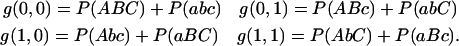
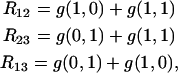
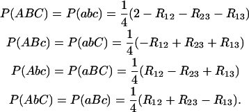
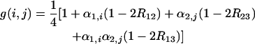
Abstract

We consider fixed recombinant inbred lines (RILs) derived either by selfing or by full-sib mating; when applicable, we also consider intermated recombinant inbreds (IRIs). First, we show that the usual estimate of recombination fraction based on RIL data is biased, and we provide an estimate where the major part of that bias is removed. Second, we derive simple formulas to compute the frequencies of genotypes at three loci in RILs. We describe the nonindependence of multiple recombinations arising in RIL recombination data even though there may be no interference in each meiosis. Finally, we give formulas for interference tests, gene mapping, or QTL detection in RIL populations.

RECOMBINANT inbred lines (RILs) can be derived either by repeated selfing or by repeated brother–sister mating of the progeny of an initial F₁ cross between two inbred lines. Such populations constitute a material of choice for geneticists and breeders. First of all, the genetic material is fixed if the number of selfing or brother–sister mating generations is large enough; indeed, the chance that any given locus is heterozygous decreases very fast with the number of generations of inbreeding, and in practice 7–10 generations are sufficient. With such fixed genotypes (ignoring mutations), a line can be multiplied while staying identical, allowing measurements in different conditions virtually an infinite number of times. Second, because of the accumulation of crossovers appearing at each meiosis with every generation, the proportion of recombinant zygotes in RILs (i.e., the probability that two linked loci have different parental alleles) is higher than what it would be in the F₂. The main disadvantage of RILs is that they require long and sometimes costly procedures to develop. However, this has been tackled recently by large community efforts, for example, in mouse (Threadgill et al. 2002; Complex Trait Consortium 2004) and in maize (Maize Mapping Project, http://www.maizemap.org/). Concomitantly, the analysis of RIL data has also experienced a renewal of interest from the theoretical standpoint (e.g., Broman 2005; Teuscher et al. 2005). This article wishes to improve the statistical description of such data.

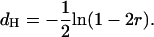
Hereafter and classically, the recombination rate per meiosis is denoted r, while the proportion of recombinant zygotes in RILs is denoted R. The relationship between r and R for two loci in fixed RIL populations derived either by self-fertilization or by full-sib matings is well known since the often-cited work of Haldane and Waddington (1931):

(1a)

or

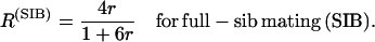(1b)

Recently, these formulas have been generalized to cope with more complex inbreeding designs (Winkler et al. 2003; Zou et al. 2005); for example, Winkler et al. (2003) extended these formulas to intermated recombinant inbred (IRI) lines having t generations of random mating prior to selfing. In a large (infinite) population, they showed, for instance, that SSD leads to

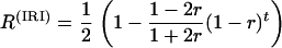(2)

and an analogous equation in the case of sib mating. Some of the work presented here applies to those cases too.

The formulas of Haldane and Waddington (Equations 1) have been the basis for linkage analysis in RILs (for genetic mapping and QTL detection). In particular, to our knowledge, they are the only core formulas used by genetic mapping and QTL detection software to accommodate data from recombinant inbred lines; this is the case not only for the oldest and still most used software, Mapmaker (Lander and Green 1987; Lander et al. 1987), but also for more recent programs (e.g., Chabrier et al. 2000; Manly et al. 2001; Wang et al. 2003). In those data analysis programs, RIL data are handled as if they were backcross data, i.e., produced by a single meiosis, except that r is replaced by R to partly account for multiple-generation effects in RILs.

Our starting point is the fact that the two-locus Equations 1 are insufficient to fully describe recombinations in RIL data; this fact has sometimes gone unnoticed or has been simply neglected because it complicates the data analysis. Indeed, through the accumulation of meioses in RIL, with either selfing or full-sib mating, the recombinations in two marker pairs are no longer independent events, even if there is no interference in recombinations during each meiosis. As a consequence, the computation of genotype frequencies at three or more loci (multipoint analysis), which enters into genetic mapping (e.g., for gene ordering) and into QTL detection (e.g., interval mapping), is more complicated with RIL data (i.e., as a function of the R's) than it is in F₂ or backcross populations (as a function of the r's). Another problem arises from the nonlinearity of Equations 1: because of that, their direct use does not provide an unbiased estimate of r.

Here, we provide new formulas that describe the statistics of RIL data. The presentation is organized as follows. First we treat the bias in the estimate of r in terms of the observed value of R. Second, we derive the formulas giving the three-locus genotype frequencies in terms of the R's. Finally, we show how these frequencies can be used in statistical inference, namely for gene mapping, to test for interference or for QTL detection by interval mapping in RILs.

GENERAL FRAMEWORK

Here, we adhere to clear and consistent definitions of recombination rate and map distance, as was the case in the original literature on linkage (e.g., Haldane 1919; Haldane and Waddington 1931), and avoid the confusion in terminology that has arisen in more recent literature. In particular, we ban the terms apparent recombination rate, apparent interference, map expansion, and equivalent distance. The recombination fraction r is defined as the expected proportion of recombinant gametes following exactly one generation of meiosis. Map distance is defined as the mean number of crossings over per meiosis in the interval of interest. There is only one map, and the size of the genetic map does not depend on the mating system or number of generations of recombination (if the map was dependent on mating system then we would need different maps for different systems). From an estimation standpoint, we estimate map distance from an estimated recombination fraction. Interference is used to describe the fact that there is a biological limitation on crossing over during one meiosis, such that crossovers are not independent. As we show, there is no pseudocrossing over occurring in a single generation that results in anything equivalent to multiple generations of recombinations. Even if there is no interference during meiosis, the fractions of recombinant zygotes in RILs (which involve multiple generations of meiosis) are not independent from interval to interval. These clarifications were greatly inspired by the comments of one anonymous referee (personal communication).

For completeness, we recall the principle behind RILs. Starting with F₁ individuals obtained from a crossing of two homozygous parents, one generates offspring either by selfing (SSD in plants) or by full-sib mating if selfing is not realizable. These offspring will fix (become homozygous) at all the loci after “enough” generations. One can also consider IRI lines: these differ from RILs in that the F₂ population is first randomly mated for t generations, and only then does one perform the inbreeding; this intermediate phase of panmixia has the effect of reducing the linkage disequilibrium among the loci. Most of this article presents results in the framework of RILs, but the generalizations to IRI lines are conceptually straightforward.

For all our work, we assume that we are dealing with diploid organisms. The probability of recombination between loci 1 and 2 during one meiosis is r₁₂. As is usually assumed, this probability is taken to be independent of the genotype and thus is the same across the different generations of the inbreeding.

Consider now the genotype frequencies in fixed lines derived from (homozygous) parents. Since we are considering only fixed lines, for notational simplicity and without loss of generality, we denote the genotypes using only one allele per locus, that is:

(3)

(4)

For two loci, these genotypes are of the form “recombinant” (Ab or aB) and “nonrecombinant” (AB or ab). As usual, one defines R₁₂ to be the probability of producing a recombinant zygote. R₁₂ is thus also the expected fraction of such lines. The definitions of r₁₂ and R₁₂ are always the same regardless of the mating system or design. However, the dependence of R on r does vary with the mating scheme (see the examples in Equations 1 and 2 above). Hence, whenever possible, we express our results directly in terms of R.

When alleles are fixed (large enough number of generations of inbreeding), the four two-locus genotypic frequencies are determined completely by the (single) recombination fraction R₁₂. We use the notation whereby g(0) is the total frequency of genotypes with no recombination (AB/AB or ab/ab), while g(1) is that of those with recombination (aB/aB or Ab/Ab). In the absence of anomalous segregation, the different genotypes in a given category are equiprobable. Obviously, g(0) + g(1) = 1; since R₁₂ = g(1), all genotype frequencies are given in terms of g(1) = R₁₂ and g(0) = (1 − R₁₂).

TWO-POINT STATISTICS

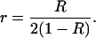
Since this whole section concerns only two loci, we drop for now the subscripts 12 on r and R to lighten the notation. Now in practice only a finite number N of lines are produced, and from these one must get estimators of the previously defined parameters, namely R = R₁₂ and r = r₁₂. The estimator of R is just the fraction of recombinant zygotes observed among the N lines, but for estimating r we have several possibilities.

Bias reduction in the case of RILs by SSD:

First we consider the case of a sample of N fixed recombinant inbred lines derived independently by single-seed descent from the starting F₁. The number of times each genotype arises is stochastic; we are principally interested in the number m of recombinant lines; and m is a random variable, of distribution

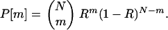(5)

Maximization over R of the likelihood of the given data leads to the obvious estimator :

(6)

As expected, this is the number of recombinant lines divided by the total number of lines.

An estimator of a quantity is unbiased if the expectation of that estimator equals the exact value of the quantity. The starting point of our discussion here is that although is unbiased, this is not the case for the “usual” estimator of r (e.g., in Mapmaker, see Lander and Green 1987; Lander et al. 1987). This usual estimator, obtained by plugging instead of R into the Haldane–Waddington equation (Equations 1) and solving for r, has a bias of order 1/N; the source of this bias is the fact that the relation between r and R is nonlinear. Let us look at this more carefully.

The expectation of can be computed, using the binomial distribution of m; one obtains

(7)

This shows that is an unbiased estimator of R.

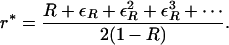
We are interested in estimating r; inverting (1a) gives

(8)

The simplest and often used estimator of r is 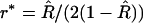; however, this estimator turns out to be biased. An intuitive explanation of the origin of this bias is as follows. Assume that r and R are the true values linked by Equation 1a. Because is unbiased, it can be thought of as the sum of the true value plus a random noise of zero mean: However, because the relation (1a) is not linear, it is easy to see (e.g., graphically) that using (1a) to project the distribution of noisy -values on the r-axis leads to a distribution that is not centered on the true value r. Hence E[r*] ≠ r (indeed E[r*] > r) so r* is a biased estimator of r.

To quantify this mathematically, first rewrite the estimator as

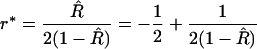(9)

and then perform the Taylor series expansion in :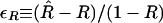

(10)

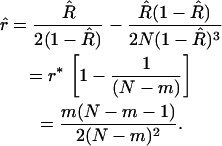
Now we take expected values: using the fact that is unbiased, we have

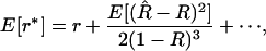(11)

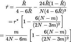
where the higher-order terms are associated with higher-order moments of . Although this formula assumes that one knows R, it is nevertheless useful. First, to this order in the Taylor expansion, we can replace 1/(1 − R) by . Second, although the expectation depends implicitly on R, we can estimate this variance assuming that the value of R = : the result is . This approach then leads us to a modified estimate for r in which most of the bias has been removed:

(12)

Although this new estimator is still biased, the remaining bias is now only of order 1/N². It is possible to obtain higher-order corrections, either by keeping more terms in the Taylor expansion or by appealing to strategies from inverse problem methods (Bako and Daboczi 2002).

Bias reduction in the case of RILs by SIB:

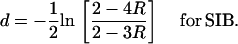
The same kind of analysis can be applied to the case of recombinant inbred lines derived by full-sib matings. This modifies the relation between r and R (cf. Equation 1b); solving Equation 1b for r leads to

(13)

As in the previous discussion, the obvious estimate of R is given by (6) and is unbiased. But, plugging that estimate into the formula for r leads to an estimate 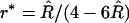with a bias of order 1/N for N lines. To remove the leading bias, one proceeds just as described before; the derivation is straightforward so we simply give the result here:

(14)

General case and application to IRI lines:

So far we have considered recombinant inbred lines only but more general designs such as IRI lines can also be treated. The definitions of and R are the same as before (just use the fraction of recombinant zygotes) and again is unbiased. From these quantities, we want to estimate r. The main difficulty comes from the fact that r is not known analytically as a function of R: one has to resort to a numerical determination of r*. For instance, in IRI lines, (2) cannot be inverted to give a closed-form expression for r = f(R); instead, r will be obtained numerically to arbitrary accuracy. A priori, this difficulty makes computing the bias problematic; nevertheless, it can be done, albeit at the cost of long formulas.

Rather than consider the particular case of (2), let us treat the general case of an arbitrary relation between R and r, represented as r = f(R). The straightforward estimator for r is . Unless f is linear, this naive estimator of r is biased. As in the case treated before, the bias can be computed formally from the Taylor series expansion:

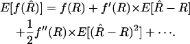(15)

Since is unbiased, the expectation vanishes and the leading bias in the estimator for r comes from the variance of . As discussed in the previous section, although we do not know this variance exactly, its value to leading order in 1/N is . Similarly, we can replace f(R) by to this order, so that our corrected estimator is

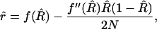(16)

where is the second derivative of f evaluated at the point .

A technical difficulty arises when applying this formula: if f is known only through its inverse f⁻¹ (as is the case with IRI), the computation of the f″ term has to be indirect. Rather than tabulating f (numerically determining it at a series of points) and then taking its second derivative that numerically introduces discretization errors, we observe that f″ can be expressed in terms of the derivatives of f⁻¹. The advantage of such an approach is that one circumvents any root solving problems. The mathematics are relatively simple and start with the relation between the derivatives,

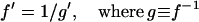(17)

is introduced to lighten the notation. Differentiating once more leads to

(18)

This thus leads to a simple computation of once the term r* has been extracted. The bias of is again of order 1/N².

The case of IRI lines can be treated directly with this approach. First, the naive estimator of r has to be obtained by solving (2) numerically; let r* be the value so that ; this gives the first term on the right-hand side of (16). Second, using (18), one computes f″ via g and its derivatives (which are known explicitly); this gives the second term on the right-hand side of (16). The final result is a modified estimator in which the O(1/N) bias has been removed.

THREE-POINT STATISTICS

Three-locus genotype frequencies:

We consider now fixed RIL or IRI lines with three loci. There are eight genotypes denoted ABC ≡ ABC/ABC, aBc ≡ aBc/aBc, etc., in the obvious fashion. In the absence of anomalous segregation, the eight genotype frequencies depend only on whether there are or are not recombinations in the intervals 1–2 and/or 2–3, so the problem reduces to finding four quantities. Let g(i, j) denote the probability of obtaining genotypes with i (0 or 1) recombinations between loci 1 and 2 and j recombinations between loci 2 and 3. We thus have

(19)

Since

(20)

the knowledge of the three recombination rates R₁₂, R₂₃, and R₁₃,

(21)

suffices to determine all genotype frequencies by solving the system of linear equations formed by (20) and (21). This gives

(22)

These equations can be summarized via the general formula

(23)

with

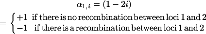(24)

and the same for α_2,j, locus 2, and locus 3, respectively.

An intuitive demonstration of (22) can be obtained using Table 1 and Figure 1 as follows. Because we assume that the three loci 1–2–3 are linked on the genetic map, there is a strict dependency of the recombination events in the interval 1–3 on the recombination events in 1–2 and 2–3. These dependencies are shown in Table 1. Then, in the Venn diagram in Figure 1, the sets and , corresponding to recombination events in 1–2 and 2–3, respectively, are sufficient to divide the space into four mutually exclusive subsets, each corresponding to one frequency g(i, j) (also indicated in the figure). From basic set theory, R₁₂ + R₂₃ − R₁₃ = 2g(1, 1); similarly, g(1, 0) = R₁₂ − g(1, 1), etc., from which one obtains the relations (22). It is nice to note that the coefficients of the R's in (22) are exactly the signs given in Table 1, where (+) corresponds to recombination and (−) to no recombination.

TABLE 1.

Allowed joint recombination events between three loci

Recombination in interval
1–2	2–3	1–3
No (−)	No (−)	No (−)
No (−)	Yes (+)	Yes (+)
Yes (+)	No (−)	Yes (+)
Yes (+)	Yes (+)	No (−)

Figure 1.

Venn diagram showing the different recombination events and the corresponding genotype frequencies.

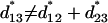
Although genotype frequencies can as well be expressed in terms of the r's, there are three nice features of Equations 22 that come directly from the fact that we express genotype frequencies in terms of the R's, as long as each R is defined as in (6): (i) Equations 22 hold for any mating system (RIL by SSD, RIL by full-sib matings, IRI, …); (ii) Equations 22 make no assumption about interference in each meiosis, and hence they hold whether or not there is interference; in fact, if there is interference, its effects are already incorporated into the R's; and (iii) Equations 22 are compact and general for any values R₁₂ ≠ R₂₃, while the same relations in terms of the r's are more complex so that only the restricted case r₁₂ = r₂₃ has been published in extenso so far (e.g., Broman 2005).

Note that since the three pairwise recombination fractions determine all genotype frequencies, necessarily the probability of double-recombinant zygotes is always given in terms of the probabilities of the single-recombinant zygotes.

Distances and mapping function:

Relation between recombination rates:

Now we can ask what the relation is between R₁₂, R₂₃, and R₁₃. This will indeed depend on possible interference between the recombinations. Assuming here that there is no interference in the crossover events during meiosis, we have

(25)

or

(26)

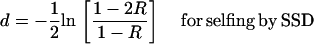
For RIL with SSD, one has R = 2r/(1 + 2r); expressing (26) in terms of the R's then gives the relation

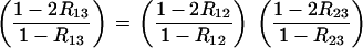(27)

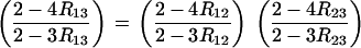
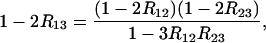
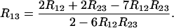
This can be transformed into explicit relations for R₁₃,

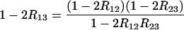(28)

or

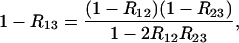(29)

giving

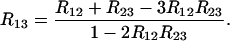(30)

In the case of sib mating, given the relation R = 4r/(1 + 6r), the assumption of noninterference gives

(31)

Solving for R₁₃ leads to

(32)

which generalizes very elegantly the SSD formula; this can also be put into the form

(33)

Unfortunately, within IRI lines, the relation between R and r cannot be solved explicitly for r if t > 3; because of this, we have no simple relations between the R's, be it for SSD or for sib mating.

Additivity of distances:

Both RIL and IRI lines have the effect of increasing the fraction of recombinant zygotes for the simple reason that there are multiple meioses. Many authors have interpreted this as a “map expansion” phenomenon (see Teuscher et al. 2005 for a recent example). However, such a term is misleading: there is a single map, and using the R's instead of the r's does not lead to a new map. The appropriate interpretation is that the N RIL or IRI lines provide higher map resolution than N separate meioses.

It seems useful to clarify once and for all these points. Recall that the distance between two loci is defined (in morgans) to be the mean number of crossings over arising in that interval during a single meiosis (such distances are then necessarily additive). Generally one does not know the number of crossings over but only its parity, an odd (resp. even) number giving (resp. not giving) a recombination between the two loci under consideration. This difficulty then pushes one to infer distances from recombination rates. In the case of no interference in each meiosis, we can make everything explicit. In that case, the distance d_H is given in terms of Haldane's map function:

(34)

Naturally such distances are additive. However, when simply plugging R into (34) one does not get a map function. Namely, the quantity

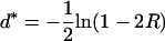(35)

is not additive: for three loci 1–2–3 we have

(36)

as can be checked from (28) or (32).

To compute genetic map distances from the R-values, write (34) in terms of R, which gives

(37a)

or

(37b)

Distances can thus be estimated either at the single-meiosis level (via r) or at the RIL level (via R).

Testing locus order in RIL:

One can use the three-locus frequencies in (22) for ordering three loci in mapping problems. The problem is to find the most likely ordering of the loci given the recombination rates. We focus on RIL and IRI lines, working directly with R-values. Consider that a finite number N of fixed lines are produced; we denote by n_i,j the number of lines with i recombinations in the first interval and j in the second. Given the property of independence of the lines, the joint probability of having generated n_0,0, n_0,1, n_1,0, and n_1,1 such lines is

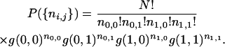(38)

This probability is, via the g's, a function of the R's, but note that a choice has been imposed implicitly for the “middle” locus. There are three possibilities for this middle locus, and for each such choice, one is to find its likelihood.

In what follows we assume that there is no interference. The maximum-likelihood approach is to maximize over all choices of the R's; this provides estimates of the R's and avoids referring to an a priori distribution. Since we assume there is no interference, we can eliminate R₁₃ by reexpressing it in terms of R₁₂ and R₂₃. This step uses explicitly the SSD or sib-mating assumption [cf. relations (30) and (33)]. Performing it is straightforward for RI lines but not for IRI lines; indeed R₁₃ is not known analytically in that case and so one must resort to doing the elimination numerically. For that, one computes r₁₂ and r₂₃, then r₁₃ = r₁₂ + r₂₃ − 2r₁₂r₂₃, and finally R₁₃ via the explicit IRI formula.

Maximizing the likelihood over R₁₂ and R₂₃ requires searching in a two-parameter space with an allowed domain 0 ≤ R ≤ 0.5. This search can be done numerically. Performing this search for the three possible orderings then leads to the order with the largest maximum likelihood.

Note that the parameter settings and that maximize the likelihood in general will be different from the values estimated from two-locus data only as additional information has been included. This is not the case when one single meiosis is involved (e.g., backcross) in which case the two and three-locus estimates of the recombination fractions are the same. This property can be traced back to the fact that the recombinations in each interval are independent in one meiosis. However, this is not the case in RILs and so it is mathematically more justified to infer locus order by simultaneously using all the three-locus data. A more naive method consists of using first the data for each interval separately to extract the R's and then using this in (38) to get a likelihood for each of the orderings. We implemented the algorithms for these two approaches but in practice we found that they lead to essentially identical results.

Interference in RIL:

Nonindependence of recombinations:

Equations 30 and 33 were derived assuming no interference at each meiosis. Nevertheless, it is clear that the relation between the R's is not the same as the one between the r's (see Equation 25), namely

(39)

Hence, recombinations in different intervals are not independent events in RILs, even if there is no interference at each meiosis. We quantify here the amount of nonindependence in RIL data (when there is no interference in each meiosis) by the four ratios:

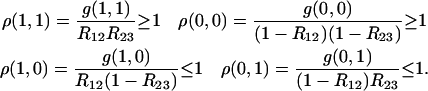(40)

Hence, compared to what would be obtained if genotype frequencies in RILs could be computed as if they were produced by a single pseudomeiosis (where r would be replaced by R), we see that there are more double-recombinant zygotes and nonrecombinant zygotes and fewer single-recombinant zygotes. Furthermore, the relative excess of nonrecombinant zygotes is small, much smaller than the relative excess of double-recombinant zygotes.

To illustrate this point, we show in Figure 2 these ratios when R₁₂ = R₂₃ = R as a function of R. The deviations from independence for double-recombinant zygotes is highest when R is small, and there ρ(1, 1) tends to 1.5 (hence the frequency of double-recombinant zygotes is as much as 50% higher than that given by the product R₁₂ R₂₃ for small R) while at large R the RIL recombinations become independent as expected. In Figure 2, we also show the two other ratios related to nonindependence for nonrecombinant and for single-recombinant zygotes; note that the former departs very little from 1.

Figure 2.

Ratios of true three-locus genotype frequencies to those obtained neglecting recombination correlations, in the case R₁₂ = R₂₃ = R (cf. Equations 40). The largest deviation from 1 is for the double-recombinant zygotes [ρ(1, 1)], and the smallest is for the nonrecombinant zygotes [ρ(0, 0)].

Test of true interference:

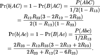
It can be of interest to consider the consequences of true interference at each meiosis so let us see how to test this directly from RIL data using Equations 22, applying standard linkage analysis methods developed for other crosses (Ott 1999, pp. 124–128). Generalizing the test on the basis of the coefficient of coincidence in individual meioses (Muller 1916), we consider the ratio

(41)

where “no interference” is the result when crossing-over events are independent; this corresponds to taking R₁₃ as given in (30) when computing g(1, 1). A simple calculation in SSD then gives

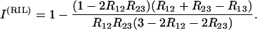(42)

In analogy with Strickberger (1985), interference is quantified here by I^(RIL), so that absence of interference gives I^(RIL) = 0. Note that in general the tests of interference based on such double-recombinant zygote frequencies have a low power (Elandt-Johnson 1971; Ott 1999).

It is also possible to consider validating a particular model of interference. Then one should consider the ratio of actual recombinant zygote frequencies to theoretical ones, using for the “theory” the model's value for R₁₃ in terms of R₁₂ and R₂₃.

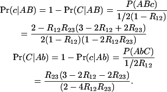
Conditional genotype frequencies:

The last application of Equations 22 that we provide is the computation of the conditional probability of the (unknown) genotype at one of the three loci, given the (known) frequencies of genotypes at the two other loci. This is relevant in particular for the two cases below. Note that we assume no interference here.

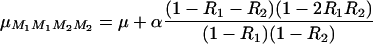
QTL detection:

In QTL detection by interval mapping, one tests for the effect of a putative locus Q/q in the interval between two markers M₁ and M₂. Setting M₁ ≡ A, Q ≡ B, and M₂ ≡ C to keep to our notations, the relevant conditional probabilities to perform QTL detection in RILs are

(43)

Hence, considering that the QTL has an additive effect α, so that QTL genotypic values are μ_QQ = μ + α and μ_qq = μ − α, the mean values for the flanking markers genotypes are

(44)

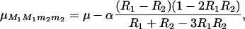(45)

where R₁ is the recombination rate between M₁ and Q, and R₂ is that between Q and M₂ (R₁₂ and R₂₃, respectively, in our notations). The means for the two other marker genotype classes are obtained by symmetry, so finally, the “marker effect” that can be estimated by linear model approaches [] is the second term of (44). Numerical evaluation of this quantity shows that approximating genotype frequencies in RILs “as if” they were produced by a single pseudomeiosis where r would be simply replaced by R leads to an overestimation of QTL effects of ∼2% as soon as M₁ and M₂ are >20 cM apart.

Missing data in genetic mapping:

Our second example is the treatment of missing data in genetic mapping software. When genotyping data are missing for some individuals at some markers, rather than simply dropping the individual/marker, one may replace the missing data by their expected values given the available data at other markers/individuals, using an appropriate algorithm (e.g., Lander and Green 1987). In addition to the above conditional probabilities for the middle locus, the following probabilities for the “external” locus are also relevant:

(46)

CONCLUSIONS

We have reconsidered two- and three-locus statistics in RILs and extensions thereof, assuming all alleles to be fixed. From the two-locus recombination fraction, one can estimate the recombination rate per meiosis; removing most of the bias in this estimate can be done quite cheaply and effectively. Interestingly, the two-locus genotype frequencies completely determine the three-locus ones, independently of the design or interference model. When recombinations at the level of individual meioses are independent, we provided the formulas relating the different recombination fractions. Furthermore, we exhibited the nonindependence of recombinations in such lines. Our three-locus formulas can be used for more reliable data analysis of inbred lines, for instance, for tests such as interference detection or QTL interval mapping. Extensions of such formulas to four loci would be of interest; unfortunately, the two-locus frequencies do not determine these uniquely, because line design and interference must be taken into account.

References

- Bako, T. B., and T. Daboczi, 2002. Unbiased reconstruction of nonlinear distortions. IEEE Instrumentation and Measurement Technology Conference, May 21–23, 2002, Anchorage, AK.
- Broman, K. W., 2005. The genomes of recombinant inbred lines. Genetics 169: 1133–1146. [DOI] [PMC free article] [PubMed] [Google Scholar]
- Chabrier, P., C. Gaspin and T. Schiex, 2000. Carthagene: a maximum likelihood multiple population genetic/radiated hybrid mapping software. Plant & Animal Genome VIII Conference, January 2000, San Diego, p. 19.
- Complex Trait Consortium, 2004. The Collaborative Cross, a community resource for the genetic analysis of complex traits. Nat. Genet. 36: 1133–1137. [DOI] [PubMed] [Google Scholar]
- Elandt-Johnson, R. C., 1971. Probability Models and Statistical Methods in Genetics. Wiley, New York.
- Haldane, J. B. S., 1919. The combination of linkage values and the calculation of distances between the loci of linked factors. J. Genet. 8: 299–309. [Google Scholar]
- Haldane, J. B. S., and C. H. Waddington, 1931. Inbreeding and linkage. Genetics 16: 357–374. [DOI] [PMC free article] [PubMed] [Google Scholar]
- Lander, E., and P. Green, 1987. Construction of multilocus genetic maps in humans. Proc. Natl. Acad. Sci. USA 84: 2363–2367. [DOI] [PMC free article] [PubMed] [Google Scholar]
- Lander, E. S., P. Green, J. Abrahamson, A. Barlow, M. J. Daly et al., 1987. MAPMAKER: an interactive computer package for constructing primary genetic linkage maps of experimental and natural populations. Genomics 1: 174–181. [DOI] [PubMed] [Google Scholar]
- Manly, K. F., R. H. Cudmore, Jr. and J. M. Meer, 2001. Map Manager QTX, cross-platform software for genetic mapping. Mamm. Genome 12: 930–932. [DOI] [PubMed] [Google Scholar]
- Muller, J., 1916. The mechanism of crossing over. Am. Nat. 50: 193–207. [Google Scholar]
- Ott, J., 1999. Analysis of Human Genetic Linkage, Ed. 3. Johns Hopkins University Press, Baltimore.
- Strickberger, M. W., 1985. Genetics, Ed. 3. MacMillan, New York.
- Teuscher, F., V. Guiard, P. E. Rudolph and G. A. Brockmann, 2005. The map expansion obtained with recombinant inbred strains and intermated recombinant inbred populations for finite generation designs. Genetics 170: 875–879. [DOI] [PMC free article] [PubMed] [Google Scholar]
- Threadgill, D. W., K. W. Hunter and R. W. Williams, 2002. Genetic dissection of complex and quantitative traits: from fantasy to reality via a community effort. Mamm. Genome 13: 175–178. [DOI] [PubMed] [Google Scholar]
- Wang, J., R. W. Williams and K. F. Manly, 2003. WebQTL: web-based complex trait analysis. Neuroinformatics 1: 299–308. [DOI] [PubMed] [Google Scholar]
- Winkler, C. R., N. M. Jensen, M. Cooper, D. W. Podlich and O. S. Smith, 2003. On the determination of recombination rates in intermated recombinant inbred populations. Genetics 164: 741–745. [DOI] [PMC free article] [PubMed] [Google Scholar]
- Zou, F., J. A. L. Gelfond, D. C. Airey, L. Lu, K. F. Manly et al., 2005. Quantitative trait locus analysis using recombinant inbred intercrosses (RIX): theoretical and empirical considerations. Genetics 170: 1299–1311. [DOI] [PMC free article] [PubMed] [Google Scholar]