Immediacy Versus Anticipated Delay in the Time-Left Experiment: A Test of the Cognitive Hypothesis

Abstract

In the time-left experiment (J. Gibbon & R. M. Church, 1981), animals are said to compare an expectation of a fixed delay to food, for one choice, with a decreasing delay expectation for the other, mentally representing both upcoming time to food and the difference between current time and upcoming time (the cognitive hypothesis). The results of 2 experiments support a simpler view: that animals choose according to the immediacies of reinforcement for each response at a time signaled by available time markers (the temporal control hypothesis). It is not necessary to assume that animals can either represent or subtract representations of times to food to explain the results of the time-left experiment.

According to the prevailing cognitive theory of interval timing, animals encode temporal events along a linear subjective time scale (Gibbon, 1977, 1991). The time-left experiment (Gibbon & Church, 1981) has played a pivotal role in advancing this view and in extending it to explain choice in animals (e.g., Brannon, Wusthoff, Gallistel, & Gibbon, 2001; Brunner, Gibbon, & Fairhurst, 1994; Dehaene, 2001; Gibbon, Church, Fairhurst, & Kacelnik, 1988; Wearden, 2002). We critically examine two assumptions of the cognitive theory of timing in this article: (a) that animals in the time-left procedure choose between delayed reinforcers by calculating differences between elapsed and expected times and (b) that these calculations are based on a linear subjective time scale. We scrutinize the procedure and these claims in light of cognitive versus operant theory and provide empirical tests.

The procedure Gibbon and Church (1981) used with pigeons is illustrated in Figure 1. After an intertrial interval (ITI; usually fixed at 15 s), a trial starts with two alternative responses becoming available—for example, the illumination of left and right response keys in a pigeon chamber. These alternatives are the time-left key and the standard key. This is the initial link (IL) phase of the trial. After a variable interval (VI), T, the next response to either alternative moves the bird into the second terminal link (TL) phase of the trial that leads to food; the alternative that was not responded to is no longer available. The time-left choice is a tandem schedule (IL and TL stimuli are white keys) in which the time to reinforcement from the start of the trial is always a constant, C, so the time to reinforcement from the beginning of the second link is C − T (the time elapsed during the IL). The standard choice is a chain schedule (IL and TL stimuli are red and green keys, respectively) in which the TL time to reinforcement is a constant value, S, from the start of the second link. Given this arrangement, it is easy to see that during the VI ILs, subjects should respond on the standard choice if the time remaining in the time-left side, C − T, is greater than the standard value, S; but they should respond on the time-left IL once C − T is less than S. Figure 2 shows that this is approximately the pattern seen with rats (Preston, 1994) and pigeons (Gibbon & Church, 1981).

Figure 1.

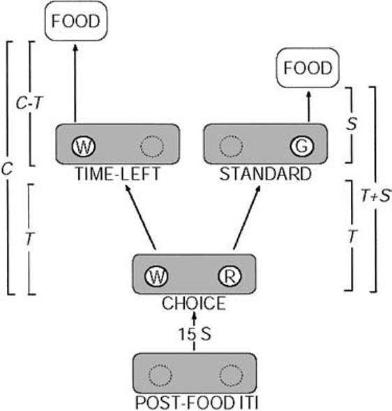
Diagram of the Gibbon and Church (1981) concurrent chain–tandem (C−T) schedule contingencies used in Experiment 1. Cycles began with the presentation of white (W) and red (R) initial-link (IL) disks. The first response to an IL after T s elapses simultaneously produced the corresponding terminal-link (TL) stimulus and removed the alternative IL stimulus. A white IL response produced a white time-left alternative, resulting in reinforcement after C − T s; a red IL response produced a green (G) standard disk, resulting in reinforcement after S s. In Experiment 1, T varied between 5 and 55 s, C = 60 s, and S = 30 s. The colors of IL and TL stimuli were varied between conditions and pigeons, as discussed in the text. T = variable IL interval; S = standard fixed delay to food; C = time to reinforcement for time-left choice; ITI = intertrial interval.

Figure 2.

Time-left preference for the 3 pigeons (P) in Gibbon and Church (1981) and for the 4 rats (R) in Preston (1994). Pigeon data are from conditions with C = 60 s and S = 30 s, as in the present study. Solid lines show predicted indifference points (relative responses equal .5), which are at the point of objective equality (C − T = S), at each value of S. (Data replotted from original figures.) T = variable initial-link interval; S = standard fixed delay to food; C = time to reinforcement for time-left choice. Left panel from “Time Left: Linear Versus Logarithmic Subjective Time,” by J. Gibbon and R. M. Church, 1981, Journal of Experimental Psychology: Animal Behavior Processes, 7, p. 98. Copyright 1981 by the American Psychological Association. Adapted with permission of the author. Right panel from “Choice in the Time-Left Procedure and in Concurrent Chains With a Time-Left Terminal Link,” by R. A. Preston, 1994, Journal of the Experimental Analysis of Behavior, 61, p. 354. Copyright 1994 by the Society for the Experimental Analysis of Behavior. Adapted with permission.

The Cognitive Hypothesis

According to advocates of the cognitive approach to timing, the time-left experiment require[s] subjects to take a difference between a current time and a future time on their subjective time scale first and then compare that difference to a standard interval. It is this preliminary differencing operation that allows different predictions for the [linear vs. logarithmic] time scales. (Gibbon & Church, 1981, p. 88)

In other words, the idea is that animals are always comparing the expected time to food on the time-left key (C − T) with the known fixed time to food on the standard key (S). Performance on the time-left task can then be used to compare the two hypothetical subjective time scales. We term this assumption the cognitive hypothesis.

The cognitive hypothesis assumes some kind of mental representation (i.e., variable) for expected time to food. The variable for expected time on the time-left key can be denoted by f(t_{T − L}), and the variable for the comparison or standard key by f(t_S), where t is real time. The assumption is that f(t_S) = f(S) and f(t_T−L) = f(C) − f(T), where C is the time to reinforcement (TTR) on the time-left side, S is the fixed duration on the standard side, and T is the IL time when the animal enters the TL.

Given this assumption, two things follow: (a) Expected times to reinforcement, f(t_T−L) and f(t_C), will be judged equal when S = C − T (i.e., when the objective times to reinforcement are equal) only if

$$f\left(C\right)-f\left(T\right)=f(C-T)=f\left(S\right),$$ (1)

that is, if the function of differences is equal to the difference of functions, which is true; and (b) only if f is a linear function. If f is logarithmic, however, Equation 1 is false.

This analysis explains why animals initially favor the standard side (C − T > S) but then switch to the time-left side as IL time, T, increases. It does not by itself account for the usual bias in favor of the time-left side seen in Figure 2: The indifference point is often before, rather than at, C − T = S (e.g., Brunner et al., 1994; Gibbon & Church, 1981). A multiplicative bias parameter, b, has to be added to the right-hand side of Equation 1 to account for this (Gibbon & Church, 1981, Equation 1).

Presented in this way, the time-left procedure seems intuitive and straightforward. But the theoretical interpretation has been questioned because it is not clear that the findings require either a differencing operation or a linear subjective time scale (Dehaene, 2001; Staddon & Higa, 1999; Staddon, Higa, & Chelaru, 1999). Dehaene (2001) has shown that behavior in a numerical analog of the time-left procedure (Brannon et al., 2001) can be modeled by a neural network that learns the best alternative as a function of linear or logarithmic time elapsed since the start of a trial with no explicit comparison (but see critique by Gallistel, Brannon, Gibbon, & Wusthoff, 2001). Staddon and Higa (1999) made a similar argument for the original time-left experiment, saying that a decaying memory trace for trial onset can serve a discriminative function for the shorter real-time delay to food as a function of the increasing IL time, T (see also Staddon et al., 1999).

In addition to problems of theoretical interpretation, the procedure also poses problems of experimental analysis. Preston (1994), in a neglected article, has pointed out that the time-left procedure makes it difficult to identify the relevant independent variables. Preference in concurrent schedules is usually thought to be determined in some way by relative reinforcement rates (Mazur, 2001; Williams, 1988). The problem is that in the time-left procedure, these rates are highly dependent on the animal's preference itself: “It is no more possible to identify the programmed relative reinforcement rates in the time-left procedure than it is to report the programmed temporal rate of primary reinforcement in a variable-ratio schedule” (Preston, 1994, p. 352). Preston demonstrated the importance of these dynamic variables with rats, finding that data (Figure 2) were well described by choice models only when they incorporated measures of empirically determined reinforcement probability (as in the generalized matching law; Davison, 1987) plus delay (as in the delay-reduction model; Luco, 1990). The following argument expands on Preston's claim by looking at an alternative account in terms of standard operant choice theory.

An Alternative to the Cognitive Hypothesis: Relative Immediacy

Any comprehensive explanation for behavior on the time-left experiment implies some kind of learning–timing process. First, animals must have some way of estimating current time, T, in each trial. Time estimation has two aspects: selection of a time marker, that is, the event that initiates timing, and some process that measures time from that point. The cognitive hypothesis has little to say about the time marker, but the usual assumption is that it is something to do with the events that signal trial onset. The hypothesis in its original form assumes a linear time-measuring process driven by a pacemaker (Gibbon, 1977, 1991). IL timing is part of all theories of time-left behavior, but not all require a linear time-measurement process.

The second, and more problematic, aspect of the process that underlies time-left behavior is the question of what is learned. The cognitive hypothesis assumes that the animal learns to anticipate the upcoming times on each side: C − T on the time-left side and S on the standard side. Thus, at each time, T, the animal is assumed to derive a variable representing (linearly) the upcoming C − T on the time-left side and the constant upcoming time S on the standard side. Choice judgments are made, according to this view, by comparison of these two variables, as in Equation 1 (above).

The key difference between the cognitive hypothesis and alternatives lies in this second factor: representation of the upcoming time. An alternative possibility is that instead of encoding real time T and remembered time C and subtracting them to get an estimate of upcoming times C − T, the animal encodes the values associated with left and right keys–alternatives at time T. This is certainly the usual way of explaining behavior on conventional concurrent schedules (e.g., Preston, 1994). Relative-response rate in the choice link is then explained in terms of the relative values of each outcome. There is no clear consensus in the operant choice literature on exactly what quantitative law determines value on concurrent chain schedules, but all agree that time to reinforcement—or its reciprocal, reinforcement rate or immediacy—plays an important role (see review in Staddon & Cerutti, 2003). Thus, an alternative to the cognitive hypothesis is the idea that what is encoded, at each value of T, is the immediacy of reinforcement associated with that time.

Expressed in the most general way, the key difference between the cognitive and relative immediacy (RI) views is just this: The cognitive hypothesis assumes that both real time, T, and upcoming (remembered) time, f(S) or f(C − T), are encoded in the same way, that is, according to the same linear scale. But the RI hypothesis permits (but does not require) real (i.e., IL) and upcoming (i.e., TL) time to be encoded differently. Real time may be encoded (as far as these data go) by any monotonic function, including an approximately logarithmic function (e.g., Staddon & Higa, 1999). But upcoming time to reinforcement may be encoded as an immediacy, that is, 1/S or 1/(C − T). Sometimes a constant, K, is added to the denominator, and in this form the RI view is known as hyperbolic temporal discounting, which has become the standard approach to choice between delayed reinforcers (see review in Mazur, 2001). In the present analysis, the function of the constant is simply to put an upper limit on immediacy when T approaches zero; it does not affect the predictions.

One uncertainty in applying the RI view to the time-left experiment is that the signals for component transition on the two sides are different. The standard side is a conventional chain schedule, but the time-left side is a tandem schedule in which the only signal for a transition from IL TL is the disappearance of the other key. What is the effect of these different stimuli? We don't know yet (we examine this question in Experiment 1). But let's begin with the simplest case and treat both choices as tandem schedules, with identical stimuli for ILs and TLs on both sides. What would a RI analysis predict in this case?

The average immediacies are as follows:

$$R_L=\frac{p_L}{D_L},$$ (2a)

and

$$R_R=\frac{(1-p_L)}{D_R},$$ (2b)

where D_L and D_R are the times to food on each side, R_L and R_R are the two immediacies, and p_L and 1 − p_L are the probabilities of responding¹ on the time-left and standard sides, respectively.

In the time-left experiment, D_R (i.e., one alternative) is equal to S and D_L = C − T. Figure 3 (upper left) shows how immediacies change for the two sides as T increases during a trial (K = 5 for all of these curves). The lines cross at 30 s (when C − T = S), but immediacy on the time-left side rises to higher values than on the standard side, simply because response-reinforcer delays approach zero on the time-left side but cannot go below S on the standard side. The inset shows response rate on the two sides as a function of T from Pigeon P3 in the Gibbon and Church (1981, Figure 10) experiment. The theoretical and experimental curves are similar. The main exceptions are the downturn in the empirical standard curve at T = 5 s (arrow) and the flat, rather than declining, theoretical standard curve; we return to these points later.

Figure 3.

Upper left panel: Immediacy as a function of time in trial, T, on the standard and time-left sides in the time-left procedure. Inset: Response rate versus T for Pigeon P3 in Gibbon and Church (1981, Figure 10), Experiment 2. Lower left panel: Relative immediacy as a function of T. Right panel: Matching prediction when time to reinforcement is on the left (D_L > D_R). T = variable initial-link interval; D_L and D_R = times to food on the left and right side, respectively; T-L = time left; qL = relative immediacy of reinforcement on the time-left alternative; pL = proportion of responding on the time-left alternative. Inset from “Time Left: Linear Versus Logarithmic Subjective Time,” by J. Gibbon and R. M. Church, 1981, Journal of Experimental Psychology: Animal Behavior Processes, 7, p. 101. Copyright 1981 by the American Psychological Association. Adapted with permission of the author.

If the two TLs are entered equally often, which will be the case if choice proportion p_L = .5, the way the RIs for the two choices change with T is illustrated for C = 60 and S = 30 by the smoothly rising solid curve in the bottom left panel of Figure 3 (compare Figure 4 in Gibbon et al., 1988). As the upper figure illustrates, the curve passes through equality when the two delays, D_L (C − T) and D_R (S), are equal at 30. But in other respects, the curve shows a bias in favor of the time-left choice: p_L = .89 when T = 60, but p_L = .35, not .11, when T = 0. The reason for the asymmetry is that the minimum TTR on the time-left side is zero, whereas the minimum TTR on the standard side is S. Note that the RI approach makes no assumptions about differencing. All that is assumed is that at any trial time, T, the animal chooses on the basis of the values of two “stored” variables representing (remembered) immediacy of reinforcement on each side.

Figure 4.

Relative time-left (T-L) responses as a function of T s in Experiment 1. Columns show data from each condition (chain–chain on the left, tandem–chain and chain–tandem in the center, and tandem–tandem on the right); rows show data from each pigeon (P). Each plot represents data from the last three sessions of a reversal in a condition; each data point summarizes data from a 5-s bin: time-left responses divided by all responses, in that bin. T = variable initial-link interval.

Dynamics

Equation 2 is the result if choice proportion is fixed at indifference. But suppose that p_L is itself determined by RI, according to the matching relation (Herrnstein, 1961). In the steady state, RI is

$$q_L=\frac{R_L}{R_L+R_R}$$ (3)

at every value of T. If D_L = D_R, then, by Equation 2, q_L and p_L are identically equal. In other words, any value of p_L generates matching, none is preferred, not even p_L = .5. But if D_L ≠ D_R, there are only two stable solutions, p_L = 1 or 0, both trivially consistent with matching. The system has a neutral equilibrium when the two delays are the same, that is, when C − T = S, and two extreme stable equilibria at all other values of T.

The process is illustrated in the right-hand panel of Figure 3 for the case where D_L > D_R, that is, when C − T > S, if time left is on the left key. The feedback function (q_L as a function of p_L, obtained by combining Equations 1 and 2 for a given value of T) is curved below the matching line (the diagonal). No matter what the starting point (A is one starting point), the obtained value of relative reinforcement rate, q_L, yields a relative-response rate, p_L, that in turn yields a still lower q_L and so on in a descending staircase that ends up at p_L = 0. Conversely, if D_L < D_R, the feedback function lies above the matching line so the staircase terminates at p_L = 1. When D_L = D_R, the feedback function lies on the diagonal, a neutral equilibrium—any value of p_L satisfies both functions. T is of course continually resetting to zero and then increasing during each trial. Thus, the system is constantly switching from the situation shown in the bottom left panel of Figure 3, which begins with a moderate preference for the standard, through a brief sojourn at indifference, to a dynamic process driving the system to exclusive choice of the time-left key. In short, the time-left procedure is inherently unstable and biased—on each trial, the process drives preference more strongly to the time-left side at the end of the trial than it does to the standard side at the beginning of the trial.

The RI analysis provides an alternative account for the following paradoxical prediction of the cognitive hypothesis (Gibbon & Church, 1981, pp. 96–97, Equations 4–6). If f in Equation 1 is logarithmic, it follows that Equation 1 can be rewritten

$$\ln \left(C\right)-\ln \left(T\right)=\ln (C∕T)=K\ln \left(S\right),$$ (4)

where K is a lumped parameter. Now suppose that both C and S are increased by the same factor, k. All this means is that a term ln(k) is added to both sides so that Equation 4 is left unchanged. In other words, the point at which the animal is indifferent between the time-left and comparison sides should be unchanged by doubling (say) the value of both S and C. This is a prediction that is both counterintuitive and counter to data. It also leaves the indifference point undefined, because it depends on the initial completely arbitrary choice for the value of S. The RI hypothesis does not make this prediction, however, because it does not assume that the “scales” for real and remembered time are the same.

Gibbon and Church (1981) failed to confirm the invariance predicted by Equation 4 and on this account rejected the hypothesis of logarithmic scaling. But their conclusion is not forced. If animals choose on some other basis than comparisons between current and remembered times—by comparing remembered immediacies, for example—no paradox arises. Thus, the Gibbon–Church data provide only weak support for the cognitive hypothesis or for linear scaling of either real or remembered time.

The RI analysis suggests (a) that under a plausible (and, we suspect, any plausible) temporal discounting analysis, the time-left procedure biases choice in favor of the time-left side and (b) that the procedure is inherently unstable, implying that it may be difficult to obtain reliable nonexclusive choice. One clear prediction of the RI hypothesis is that, given instability and bias, a likely outcome in the time-left procedure is exclusive preference for the time-left side at all values of T. This prediction seems to be contradicted by the classical outcome seen in Figure 2. One possibility is that the RI analysis we have presented is based on a choice between two tandem schedules rather than a choice between a tandem schedule (the time-left side) and a chain schedule (the standard side). Just like the cognitive hypothesis, we did not take explicit account of the signal difference between the tandem (time-left) choice and the chain (standard) (i.e., we have ignored the asymmetrical stimulus conditions associated with the two choices, one stimulus [or one plus the weak, brief stimulus provided by offset of the standard key] for time-left, two for standard). If this objection is correct, then we should expect an effect of changing stimulus configurations. In Experiment 1, we therefore studied the effects of the three other stimulus arrangements in the time-left procedure to see whether behavior under these conditions better fits the cognitive hypothesis or the RI hypothesis. In Experiment 2, we studied a modified time-left procedure designed as a direct and unconfounded test of the cognitive hypothesis of animal timing.

Experiment 1: Stimulus Functions in the Time-Left Procedure

The original time-left procedure has an arbitrary feature that becomes apparent once it is described in more neutral schedule-based language: It is asymmetrical. The time-left choice is a tandem schedule, the standard choice a chain. Yet the same set of response and time contingencies could be associated with both choices being chains, both being tandem schedules, or the time-left side being a chain and the standard side a tandem schedule—a total of four possibilities. Even in the absence of any theoretical reason to do so, it is obviously worth studying these four arrangements, which we did in Experiment 1. If the results of the time-left experiments are due only to a timing process, then the stimulus arrangements should not matter.

Four pigeons were exposed in partially counterbalanced orders to a concurrent chain–tandem schedule (i.e., the Gibbon & Church, 1981, procedure), a concurrent chain–chain schedule, a concurrent tandem–tandem schedule, and a concurrent tandem–chain (i.e., the time-left side was a chain, the standard side a tandem). Response and temporal contingencies were the same in all four conditions (shown in Figure 1), reproducing those used by Gibbon and Church (1981) as closely as possible. The four conditions—chain–chain, tandem–chain, chain–tandem, and tandem–tandem—differed only in the colors of stimuli signaling ILs and TLs, as shown in Table 1.

Table 1.

Summary of Stimulus Conditions in Experiment 1

	Time left		Standard
Condition and pigeon	IL	TL	IL	TL
Chain–chain
25	Yellow	Orange	Blue	Cyan
299	Yellow	Orange	Blue	Cyan
1351	Green	Red	Yellow	Blue
1374	Green	Red	Yellow	Blue
Tandem–chain
25	White	White	Red	Green
299	White	White	Red	Green
1351	White	White	Red	Green
1374	White	White	Red	Green
Chain–tandem
25	Red	Green	White	White
299	Red	Green	White	White
1351	Red	Green	White	White
1374	Red	Green	White	White
Tandem–tandem
25	White	White	White	White
299	White	White	White	White
1351	White	White	White	White
1374	White	White	White	White

Note. IL = initial link; TL = terminal link.

Method

Subjects

Four male White Carneaux pigeons (25, 299, 1351, and 1374) served. All were between 6 and 8 years of age and were maintained at 85% of their free-feeding weights. The birds were housed in individual cages in a room with a 12:12-hr light–dark cycle where they received free access to water. All pigeons had previous experience in studies on choice and timing.

Apparatus

Pigeon chambers were constructed from plastic 24-gallon storage containers, with a plastic grid floor measuring 370 mm (width) × 460 mm (length) and a floor-to-ceiling distance of 310 mm. Pecks were recorded by a touch screen-equipped computer monitor placed in a 270 mm (width) × 200 mm (height) opening in one end of the container, with the bottom edge of the opening at 140 mm from the floor. Reinforcers consisting of mixed grain were delivered through a feeder opening, centrally located below the touch screen opening, flush with the floor. An exhaust fan on the wall opposite the screen circulated air and provided masking noise.

Stimuli were presented on a 13-in. VGA monitor equipped with a Carroll Touch Technology 13-in. infrared touch screen. Stimuli were two 9-mm disks (“keys”), 95 mm apart, and 165 mm above the floor. Pecks toward stimuli were buffered by a 1-mm clear polycarbonate sheet 5 mm from the surface of the monitor. Effective pecks breaking the infrared beams brought the pigeon's corneas 40 ± 2 mm from the monitor. The maximum x–y resolution of the touch screen was 3.15 mm on both axes; responses were sampled 40 times per second. Software recorded a peck to a stimulus when the beak broke the infrared beams and was removed. Only responses to stimuli were recorded; responses to other screen areas were not recorded and had no programmed consequences.

Procedure

The pigeons began procedures without additional training. Sessions in all conditions consisted of 60–80 repeats of the cycle shown in Figure 1. A cycle began with a 15-s ITI, followed immediately by the opportunity to respond to left and right IL stimuli. The first response on either side after T s produced the TL on that side and simultaneously turned off the alternative IL stimulus. The TL ended with the first response after either time C − T (60 s − T; time-left side) or S (30 s; standard side). The value of T was randomly selected without replacement from 1 of 11 possible multiples of 5 between 5 and 55 s, inclusive, in each block of 11 trials. If the time-left alternative was pecked, food became available for the first response after 60 − T + Δ s (where Δ is the time between setup at trial time T and the next IL key peck). If the standard alternative was produced, food was available for the first response after 30 + Δ s. Reinforcers consisted of 2-s presentations of mixed grain, and sessions ended after 80 reinforcers for Pigeon 1374 and after 60 reinforcers for the remaining pigeons.

Each pigeon was exposed to the four versions of the procedure: tandem–chain, chain–chain, chain–tandem, and tandem–tandem in a partially counterbalanced order. The stimuli associated with each link are shown in Table 1. In the tandem schedules, the transition to the TL was not signaled except for the disappearance of the other (unchosen) IL stimulus. In each condition, we reversed the key assignments on three occasions after six or more sessions (i.e., time-left on the left and standard on the right was changed to standard on the left and time-left on the right, or vice versa, in an ABAB fashion) to assess the recoverability of steady-state functional relations. Reversals were arranged after a minimum of six sessions when comparison of the average relative-response curves (as plotted in Figure 4) for the last two three-session blocks indicated that preference over all 11 values of T had stabilized. The stability criterion was subsequently computed on a daily basis until the relative-response curves showed no further change. The order and duration of conditions are presented in Table 2. To make sure that the results of the tandem–chain (Gibbon & Church, 1981) condition, discussed below, were not some kind of carryover effect attributable to using the same stimuli in several conditions, we repeated this condition with a completely new set of stimuli (a brown disk for the time-left schedule and purple and light blue disks for the standard schedule; see Table 2) at the end of the sequence of conditions shown in Table 2 and obtained exactly the same results.

Table 2.

Sequence of Conditions and Sessions Per Within-Condition Reversal of Schedules in Experiment 1

	Sequence of conditions (sessions per reversal)
Pigeon	1	2	3	4	5a
25	CC (11, 8, 6, 9)	TC (12, 16, 12, 7)	TT (15, 11, 10, 8)	CT (10, 13, 6, 6)	TC (16, 12)
299	TC (8, 11, 8, 14)	TT (19, 17, 21, 11)	CC (13, 10, 10, 8)	CT (11, 13, 8, 7)	TC (16, 12)
1351	TC (8, 11, 9, 18)	CC (11, 8, 14, 9)	TT (9, 8, 14, 7)	CT (14, 10, 6, 6)	TC (12, 8)
1374	TT (11, 8, 11, 9)	CC (12, 19, 11, 8)	TC (10, 13, 14, 16)	CT (12, 10, 6, 6)	TC (9, 10)

Note. C = chain; T = tandem.

^aSecond replication of the Gibbon and Church (1981) procedure.

Results

Stable, average, relative-response rates (computed in 5-s bins) on the time-left IL (y-axis) as a function of T (x-axis) are shown in Figure 4. The columns are labeled according to the procedure: chain–chain, tandem–chain (the Gibbon & Church, 1981, procedure), chain–tandem, and tandem–tandem. All pigeons in the tandem–chain condition showed increasing preference for the time-left alternative as T increased, but all also showed some bias in favor of the time-left side: The 50% points were all at T values less than 30 s.

The effects of the different stimulus arrangements were substantial. Only the tandem–chain condition, the original Gibbon and Church (1981) procedure, showed a reliable change in preference as a function of IL time, T, in every pigeon. The other three conditions showed either an effect of T in only 1 or 2 animals (chain–chain; P25 and possibly P299) or essentially no effect of T at all (chain–tandem, tandem–tandem). All pigeons in the chain–tandem and tandem–tandem conditions showed a strong preference for the time-left alternative.

All theoretical accounts for the data from the tandem–chain (Gibbon & Church, 1981) version of the procedure must assume some control of preference by time in trial, T. But this preference could derive from essentially random, but biased, responding on both choice keys or as a difference in time-to-first response (latency or wait time) on each side—or both (Staddon & Cerutti, 2003). If wait time on each choice is determined by TTR, then wait times on the standard side should peak to the left of the distribution on the time-left side because the minimum TTR on the standard side is less than on the time-left side. Figure 5 shows the wait-time distributions, as well as the obtained TTR distributions, for the tandem–chain procedure. The TTR distributions are more or less as expected: a sharp spike at 60 s for the time-left side and a broad distribution from 35–90 s on the standard side. As predicted, the wait-time distributions are different for the standard and time-left sides. The difference is largest for P25, which always showed the steepest change in preference as a function of T. But in all four cases, the wait-time distribution on the standard side peaks earlier than that on the time-left side.

Figure 5.

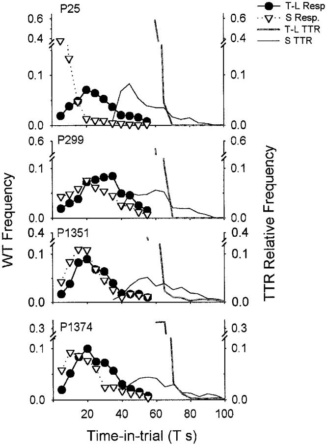
Frequency distributions of waiting and time to reinforcement (TTR) for the tandem–chain condition. Wait times (WT) are the first initial-link responses on each side. Data are averages from the last three sessions in each reversal of a condition, data are in 5-s bins, and WT and TTR data are presented as proportions of total WT and TTR counts, respectively. P = pigeon; T = variable initial-link interval; S = standard fixed delay to food; T-L = time left; Resp. = response.

Discussion

This experiment replicated the main results of the original Gibbon and Church (1981) time-left experiment. In the tandem–chain (Gibbon and Church) condition, preference for the time-left side increased with IL time, T, and there was a bias in favor of the time-left side: The point of indifference in every case was to the left of T = 30 s, the point where TTR on both sides is equal. Moreover, underlying this preference there was a strong effect of T on wait time, which conformed pretty closely to the distribution of TTRs on each side (Figure 5).

The strong correlation between relative-response rate and relative entries into the TL in all four conditions (Figure 4) suggests that local response rate was relatively constant on both sides—a result different from Preston (1994, see p. 354), who used rats rather than pigeons. Hence, changes in relative-response rate may largely reflect changes in wait time (Figure 5). Moreover, the substantial numbers of wait times in excess of 10 s accounts for the initial downturn in response rate to the standard shown in the Gibbon and Church (1981) data referred to earlier (Figure 3 inset; arrow). The reason for the declining, rather than constant, response rate to the constant-immediacy standard has to do with competition: As immediacy for the time-left choice increases, and response rate along with it, obviously less time is available to respond on the sample side.

RI makes a clear prediction of instability and exclusive time-left preference at all values of T for the tandem–tandem procedure, which was confirmed. A similar result was obtained even for two of the three differential-stimulus procedures: chain–tandem and chain–chain. Only the tandem–chain (Gibbon & Church, 1981) procedure failed to show exclusive time-left preference.

The presence or absence of differential stimuli clearly makes a difference to performance on the time-left procedure. Why is the tandem–chain (Gibbon & Church, 1981) procedure the only one to show a reliable effect of IL time, T, on preference? The simplest answer is in terms of the venerable concept of conditioned (secondary) reinforcement. Only in the chain conditions is responding in the IL reinforced by presentation of a different stimulus—a putative conditioned reinforcer—in the TL. And of these three conditions—chain–chain, chain–tandem, and tandem–chain—only the tandem–chain, the Gibbon and Church (1981) condition, is asymmetrical in a way that favors the standard side. In the IL of each chain schedule, animals may adjust their wait times to IL duration, rather than to the sum of IL and TL durations. Because the chain IL is a VI, this implies a short wait time. If the other choice is a tandem, as in the tandem–chain condition, initial responding on the chain side is favored (cf. Figure 5 in this article and Figure 10 in Gibbon & Church, 1981). As time elapses, however, the tandem (time-left) TTR approaches zero, encouraging switching to that side. The result is a change in preference to the time-left side as T increases. In the chain–tandem condition, conversely, this process favors the time-left side. With the time-left side favored both early and late, a strong T-independent time-left preference is to be expected and was found.

Chain–chain, the only condition in which some conditioned-reinforcement effect is possible on both sides, is the only other condition that shows any effect of T on preference. The effect is small and limited to 1 or 2 of the 4 pigeons. The main result in this condition, as in the tandem–tandem and chain–tandem conditions, is a strong time-left preference. But the chain–chain condition does resemble a familiar operant choice procedure: choice between concurrent-chain fixed-interval (FI) and concurrent-chain VI schedules. In the time-left procedure, both IL VIs are the same. The time-left key is the VI TL option, and the standard key the FI. By design, the mean VI interfood interval is equal to the FI value. The standard result, in a comparison between equal (arithmetic mean) FI and VI TLs is, of course, strong preference for the VI (Killeen, 1968), here the time-left key.

Finally, we note another way to look at the immediacy asymmetry illustrated in Figure 3 (left panels): delay of reinforcement. As time T increases, switches to the time-left key may be followed by food after very short delays. Switches to the standard key, however, are never followed immediately by food; the delay there is always at least 30 s. The procedure in effect enforces an asymmetrical changeover delay. This feature operates on all but the tandem–chain and chain–chain versions, where short response → conditioned-reinforcer delays are possible on the standard side.

Thus, the RI hypothesis can account for the exclusive time-left preference seen in all but the tandem–chain (Gibbon & Church, 1981) version of the time-left experiment. With the addition of an assumption about conditioned reinforcement, the RI hypothesis is consistent with data from all four conditions. The cognitive hypothesis can account for T-dependent preference in the tandem–chain condition but not (without an ad hoc added parameter) for the time-left bias. The cognitive hypothesis makes no prediction about the instability of the time-left procedure and cannot account for the exclusive preference in three of the four versions of the procedure. We conclude, with Preston (1994), that “the time-left procedure is poorly designed as a preparation for studying choice and timing” (p. 350). Because the focus of this study is the cognitive hypothesis, rather than the time-left procedure per se, in Experiment 2 we studied a procedure that allows a more direct comparison between the cognitive hypothesis and RI.

Experiment 2. Choice Between Different Times to Reinforcement Signaled by Different Time Markers: A Modified Time-Left Procedure

As we pointed out earlier, two processes are involved in time-left performance: a process that measures real time, T, and a process that encodes something about upcoming reinforcement: what is learned. In Experiment 1, we contrasted two views of what is learned: a linear time difference or immediacy. The timing process was irrelevant. In Experiment 2, we look more closely at the role of the timing process, which has two aspects: the process of timing itself and the time marker that initiates it. A principle that has been standard in operant analyses of temporal schedules for many years is that under most conditions, the pigeon's behavior is determined at any instant by the immediacy of primary reinforcement at that time, where time is measured from the most recent time marker (e.g., Shull, Mellon, & Sharp, 1990; see Staddon, 1972, for an early review). We term these two aspects—timing plus learned immediacy (the RI hypothesis)—taken together the temporal control hypothesis. In this experiment, we contrast predictions of the cognitive hypothesis and the temporal control hypothesis.

In the version of the time-left experiment used in Experiment 1, the time marker is the set of events associated with trial onset. Thus, on the time-left side, TTR signaled by trial onset is just C (60 s in Experiment 1). But on the standard side, TTR is in effect a VI schedule with minimum 35 s and maximum 85 s (S = 30 and T varied between 5 and 55 s in the original study; see Figure 5). Hence, we would expect animals to begin each trial by responding on the standard side (minimum TTR = 35 s vs. 60 s on the other side) and then later to switch to the time-left side.

But a little reflection shows that this analysis is not quite right. The standard side is not really a simple VI schedule, because the interreinforcement interval is determined not by postreinforcer (or posttrial) time, but by postresponse time, that is, it is programmed according to a response-initiated-delay (RID) schedule² (Wynne & Staddon, 1988). (In the usual RID schedule, a single response is required to initiate the delay. On the standard side in the time-left experiment, however, a variable delay, the VI schedule, is imposed before a response is effective.) A well-known property of RID schedules is that waiting time (time to first response) is always longer than on a comparable FI schedule. For example, the linear-waiting approximation (Wynne & Staddon, 1988) is that waiting time, t, on FI x is t = ax, but waiting time on RID x (i.e., a delay of x initiated by a single response) is t = ax/(1 − a), where a is a constant less than one. Thus, linear waiting alone, without taking into consideration the asymmetric immediacies illustrated in Figure 3, predicts that the indifference point in the time-left experiment should favor the time-left side (i.e., be at a T value less than C/2). Nevertheless, overall the cognitive and temporal control views make relatively similar predictions for the Gibbon and Church (1981) procedure in Experiment 1, although the temporal control view implies the observed time-left bias and can explain the tendency to exclusive choice under some stimulus conditions. Because both views make similar predictions and because of the asymmetry of the original time-left design, it is not ideal for deciding between the two views. We therefore devised a new procedure to compare the two hypotheses explicitly.

Cognitive Hypothesis

The cognitive hypothesis states that animals choose left or right depending on some kind of internal representation of upcoming time to reinforcement: “[I]n the time-left task, the subject compares the time left until reward on one side (the so-called comparison or time-left side) against the unvarying expectation on the so-called standard side” (Gallistel, 1999, p. 265). In other words, the subject does have a representation of TTR at each time-in-trial T and does directly compare S with C − T.

Temporal Control Hypothesis

That animals in the time-left experiment are timing from the most recent time marker (usually, but not necessarily, trial onset) and simply choosing at each instant on the basis of the RI of primary reinforcement.

Our modified time-left procedure (Figure 6) involves three response keys. At the beginning of a trial, the animal responds on a single center white key for a variable time T. The first response after T s turns off the center key and turns on two side choice keys. The red side key (time-left) signals a time C − T to food reinforcement; the green side key (standard) signals a time S to food; a peck on either side key turns off the other. Notice that both choice stimuli are paired with food, avoiding the paired- versus unpaired-with-food confound in the original time-left experiment.

Figure 6.

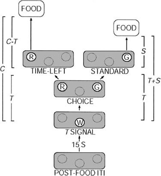
Diagram of the procedure used in Experiments 2 and 3. Cycles began with a 15-s intertrial interval (ITI) followed by a white disk (W) signaling an interval of T s. At the end of the interval, the white disk was replaced with a choice between a red (R) time-left and a green (G) standard alternative. A peck on the time-left alternative produced reinforcement after C − T s; a peck on the standard alternative produced reinforcement after S s. As in Experiment 1, T varied between 5 and 55 s, C = 60 s, and S = 30 s. The colors of initial-link and terminal-link stimuli were varied between conditions and pigeons, as discussed in the text. T = variable initial-link interval; S = standard fixed delay to food; C = time to reinforcement for time-left choice.

In this version of the time-left procedure, the animal is directly confronted by two choices, one signaling time left, C − T, the other the “unvarying expectation” of S s to food. The cognitive hypothesis predicts (a) that preference will vary as a function of the IL time, T, when the choice stimuli appear and (b) that the animals should be indifferent at the objectively equal point, where S = C − T. But the temporal control hypothesis makes three possible predictions, depending on which stimulus or combination of stimuli the animal uses as a time marker.

(a) Temporal Control by Trial Onset

In this case, responding will be governed by the posttrial-time distribution of reinforcers, which corresponds to FI 60 on the time-left side and an arithmetic VI with intervals from 35–85 s (in the all condition; see below) on the standard side. The shorter minimum interval on the standard side should lead to some initial bias to that side, and preference for the time-left side should increase as a function of T.

(b) Temporal Control by Choice-Stimuli Onset

In this case, behavior after the appearance of the two choice stimuli should be determined entirely by the poststimulus distribution of TTRs. This distribution corresponds to an arithmetic VI with intervals ranging from 5–55 s on the time-left key (in the all condition) and to an FI 30 on the standard key. Thus, wait times should be shorter for the time-left key than for the standard key. Because the first response on either key turns off the other key, the shorter time-left wait time implies a strong apparent preference for the time-left key. If temporal control is exerted only by the choice keys, there should be no effect of T on preference.

(c) Mixed Temporal Control

Mixed temporal control is some temporal control by both trial onset and the onset of the choice stimuli, that is, (a) and (b). In this case, there should be a bias in favor of the time-left key, because of control by postchoice-stimulus time; but also an increasing tendency to choose the time-left key as T increases.

These three predictions are logically distinct, but the empirical difference between (a) and (c) is one of degree. Possibility (a) implies relatively strong control of preference by trial time, T; possibility (c) implies relatively weak (but not zero) control of preference by T. None of the temporal control predictions are consistent with indifference at the point of objectively equal delays to food; all predict some time-left bias.

Pigeons tend to use as a time marker the most recent stimulus. For example, if, on a simple FI schedule, a not-too-brief stimulus is added halfway through the interval, most birds will cease responding until the stimulus appears and then show a poststimulus wait time more or less appropriate to the shortened interval. On the other hand, food reinforcement is highly salient and often more effective as a time marker than a comparable neutral stimulus (Staddon & Innis, 1969; review in Staddon, 1983, Chapter 12). Thus, outcomes (b) and (c) are perhaps the most likely, according to the temporal control hypothesis.

Throughout Experiment 2, C = 60 s and S = 30 s; there were three conditions that differed only in the distribution of T values: In the all condition, as just described, T varied in 5-s increments from 5–55 s. The short condition truncated the distribution of T values to 5–30 s. The long condition used only longer T values: 30–55 s. Notice that the short and long ranges overlap at T = 30.

We looked in each case at the steady-state preference for the time-left side as a function of T. If, as the temporal control hypothesis predicts, preference is driven simply by the TTR distribution, then preference at the T = 30 s point should not be equal under these three distributions. Preference for time-left should be in the order long > all > short. The cognitive hypothesis, on the other hand, has no basis for predicting any effect of TL TTR distribution on preference at a given T value. So long as the objective food delay is the same for both choices, as it is at T = 30 s, the region of overlap between the long and short distributions, preference should be the same.

Method

Subjects and Apparatus

Pigeons and apparatus were the same as in Experiment 1.

Procedure

The three-key procedure is similar in concept to the original two-key time-left procedure, and as many details as possible were retained. The three-key procedure is illustrated in Figure 6. Trials began with a 15-s ITI, during which the stimulus display monitor was darkened. At the end of the ITI, a white disk (key) signaling a VI IL, of duration T s, appeared in the lower center portion of the screen (19 mm in diameter and 165 mm from the floor). In each trial, T was selected randomly without replacement in blocks of 11 equally spaced values between 5 and 55 s, inclusive, as in Experiment 1.

The first response on the white key after T s turned it off and the two side keys (also colored disks) appeared as follows: red and green, on left and right, respectively. These two keys were 95 mm apart and 160 mm from the chamber floor. The appearance of these two keys (and the offset of the white key) signaled the choice (terminal) link. The first response to either of the choice keys turned off the other key and began timing the delay to food in effect for that choice. Operation of the feeder lasted 2 s, stimuli disappeared when the feeder was operated, and a new 15-s ITI began timing when the feeder stopped operating. Sessions ended after 60 trials.

Once the time-left key appeared, at time T, food reinforcement was presented for the first peck to it 60 − T s thereafter (VI 60 − T s: time-left TL). Food was presented immediately for a time-left peck if the pigeon had allowed more than 60 s to elapse before responding on the time-left key. On the standard key, food was presented for the first response after 30 s (FI 30 s: standard TL).

In this experiment, we varied the side assignment, time-left on the left, standard on the right, or the reverse, and the distribution of possible T values. Each side reversal constituted a within-animal replication.

Side. All pigeons began with the time-left choice on the left. In this and the remaining procedures, Pigeons 299 and 25 had a red time-left disk and a green standard disk; Pigeons 1351 and 1374 had a green time-left disk and a red standard disk. After 21 sessions of time left on the left, the sides of the choices were swapped for another 18 sessions, at which point the procedure ended. Changes in contingencies were made when visual inspection suggested all of the pigeons' choices were stable.

T distribution. There were three conditions: all, short, and long. The all condition is as just described: 11 T values ranging from 5–55 s. T for Pigeons 299 and 1351 was limited to the range of 5–30 s (short condition). T for Pigeons 25 and 1374 was limited to the range of 30–55 s (long condition). T was now sampled without replacement in randomized blocks of 6 (rather than 11) values. Table 3 shows the order of conditions and number of sessions in each.

Table 3.

Sequence of Conditions and Sessions Per Within-Condition Reversal of Schedules in Experiment 2

	Sequence of conditions (sessions per condition)
Pigeon	1	2	3	4	5	6
25	L: all (16)	R: all (14)	L: long (8)	L: short (12)	R: short (11)	R: long (9)
299	L: all (19)	R: all (16)	L: short (12)	L: long (14)	R: long (9)	R: short (8)
1351	L: all (21)	R: all (17)	R: long (9)	R: short (11)	L: short (10)	L: long (8)
1374	L: all (19)	R: all (15)	R: short (8)	R: long (12)	L: long (9)	L: short (11)

Note. L (time-left alternative on the left) = T − L on left; R (time-left alternative on the right) = T − L on right; all = T values to 5–55 s; short = T values to 5–30 s; long = T values to 30–55 s; T = variable interval.

Results

Figure 7 shows the steady-state proportion of time-left choices as a function of obtained T for the all condition and a replication (side reversal) for all 4 pigeons. Two of the birds (299, 1374) conform to outcome (b) in the introduction: a strong preference for time left and no control by T. The 2 others (25, 1351) conformed to outcome (c): They also show a strong time-left preference, but accompanied by some control by T (i.e., some responding on the standard side at short T values). Pigeon 25 showed some control by T on first exposure to the procedure (closed circles), but this decreased when the sides were reversed (open circles); Pigeon 1351 showed strong control by T on both exposures, corresponding to outcome (a).

Figure 7.

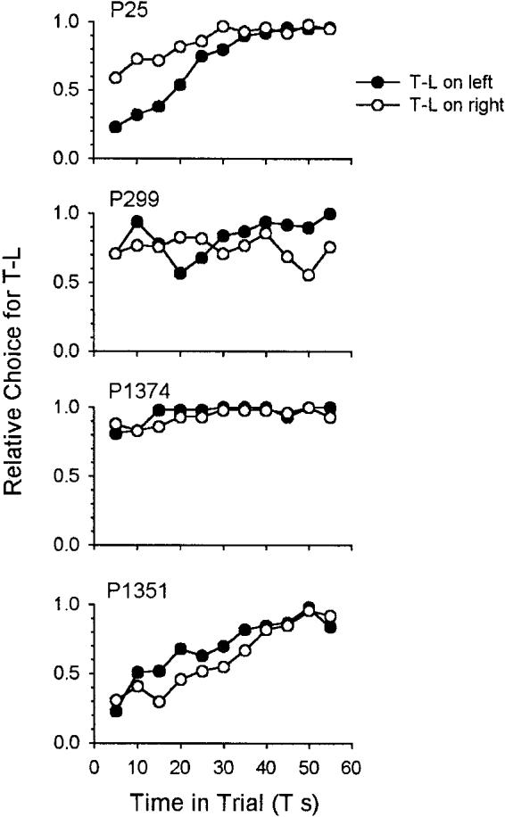
Proportion of choices for the terminal link (TL) alternative as a function of T duration in Experiment 1. Filled points are from the time-left (T-L) left condition, and open points are from the time-left right condition. Plots are data from the last 10 sessions (600 trials) in each condition. Lines are best-fitting linear functions. T = variable initial-link interval; P = pigeon.

Figure 8 shows the results from the short (triangles) and long (circles) conditions. Again, the general result is a bias in favor of time left. Control by T is shown by 1 animal in one condition (P25; short, left: filled triangles). When preference at the point of overlap (T = 30 s) can be compared between the short and long condition, time-left preference is always greater in the long condition. The preference data are a little more variable than in Experiment 1 because we had only 60 choices per session, one per trial, rather than several hundred in Experiment 1, where we could use binned response rate as a preference measure.

Figure 8.

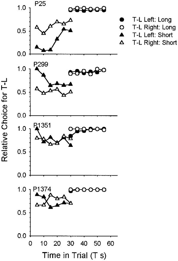
Proportion of choices for the time-left (T-L) alternative as a function of T in Experiment 2. Filled points are from the time-left left condition, and open points are from the time-left right condition; triangles are from the T-short condition and circles are from the T-long condition. Plots are data from the last 10 sessions (600 trials) in each condition. Lines are best-fitting linear functions. T = variable initial-link interval; P = pigeon.

Discussion

All of the subjects in Experiment 2 showed a strong preference for the time-left choice in the all condition. Two animals also showed some dependence of preference on the time in trial, T, at which the choice was made. These results are consistent with outcome (b), temporal control by choice-stimuli onset, the most probable outcome predicted by the temporal control hypothesis. The instances of partial control of preference by T are consistent with outcome (c), mixed temporal control by two time markers: choice-stimuli onset and trial onset.

The results of the all condition point to the distribution of times to reinforcement signaled by each choice stimulus—VI for the time-left choice, FI for the standard—as the major determinant of behavior in this situation (cf. Gibbon et al., 1988, Figure 10, who explicitly varied the distribution of sample durations in the standard time-left situation and found preference reversal: the variable-sample side was preferred over the time-left side). This conclusion gets further support from the results of the short and long conditions. When T was restricted to short values, 30 s or less, the minimum TTR signaled by the appearance of the choice stimuli, on the time-left side, was 30 s, compared with the fixed value of 30 s on the standard side. But when T was restricted to long values, 30–55 s, the minimum time-left TTR is just 5 s. These differences predict a strong time-left preference in the long condition, a weak standard preference in the short condition, and a greater preference for the time-left side at the 30-s point in the long condition. The results for all of the pigeons were consistent with the first and last predictions, but the short condition produced mixed results: some effect of T, on first exposure, combined with a bias in favor of the standard key in P25, but overall indifference on the next exposure. The other pigeons showed either indifference or a bias for the time-left side in the short condition. Neither of the predictions of the cognitive hypothesis—invariable control of preference by T and indifference at the objectively equal TTR point: T = 30 s—is supported by these data.

General Discussion

The cognitive hypothesis implies that animals trained on the time-left procedure of Gibbon and Church (1981) are performing a rather complex set of mental operations:

The subject compares the steadily diminishing time-left until reinforcement on the time-left key to the expected delay of reinforcement on a standard key. It begins a trial by pecking the standard key, because the expected delay there is shorter than the time left. The subject switches to the time-left key, when it judges the time left has become less than the expected delay on the standard key. Thus, the time left when the subject switches gives an estimate of the expected delay on the standard key. (Gallistel & Gibbon, 2002, p. 50)

This account implies that animals represent not just current time and the anticipated time of reinforcement, but can also compute the difference between those times (Equation 1, above).

The alternative is the older idea of temporal control, combined with the idea that animals choose on the basis of the (remembered) immediacy of reinforcement, a version of hyperbolic temporal discounting, which is a well-established principle of free-operant choice. Both processes appear in prototypical form in the FI “scallop.” Pigeons, rats, humans, and many other animals will adjust their response rate, or choice probability, in rough accord with the immediacy of food reinforcement at different times, where the times are measured from an effective time marker such as food delivery or the signaled onset of a trial. When food can occur at more than one posttime-marker time, pigeons will adjust both their induced activity (Staddon & Simmelhag, 1971) and their operant activity (Catania & Reynolds, 1968), accordingly, pecking or making a comparable terminal response, preferentially at times when reinforcement immediacy is high.

The temporal control hypothesis, considered in isolation, implies that because the temporal contingencies are the same, all four conditions in Experiment 1 should have produced the same result. They did not. The probable reason is that the asymmetrical stimulus arrangement in the Gibbon and Church (1981) time-left procedure provides conditioned reinforcement only on the standard side. At least three factors seem to contribute to the almost exclusive time-left preference in the other conditions of Experiment 1: (a) unstable and asymmetrical dynamics: relative immediacy, although equal when C − T = S, nevertheless favors the time-left side overall; (b) delay of reinforcement: the fact that short response-reinforcer delays are possible on the time-left side but never on the standard side; and (c) the fact that the standard side is a response-initiated-delay schedule rather than a simple VI versus the FI on the time-left side. In a comparison between RID 30 and FI 30, wait time on the RID schedule will always be longer. Even if no other factors were operating, therefore, we would expect animals to prefer FI 30 to RID 30 and would expect indifference in the time-left procedure to be closer to time left than to the point at which the arithmetic averages of the standard and time-left schedules are equal.

Time left is evidently a complex procedure not well suited for studying timing and choice. However, we were unable to demonstrate the kind of subtractive process that is claimed to occur in the time-left experiment even in the modified form studied in Experiment 2, which was explicitly designed from the cognitive point of view. Here also, the temporal control hypothesis provided a simpler and more comprehensive account of the data. Preference was determined by the distribution of immediacies signaled by the relevant time marker.

Our general conclusion is that although we cannot yet provide a precise model for what is happening in the standard time-left experiment, neither of our experiments provide any support for the cognitive hypothesis. Hence, experiments that have used this procedure to evaluate either subjective scales for time (Gallistel & Gibbon, 2002) or number (Brannon et al., 2001) cannot be taken at face value. These experiments provide no evidence either that animals use time and number scales in the ways asserted or indeed that they have scales at all.

References

- Brannon EM, Wusthoff CJ, Gallistel CR, Gibbon J. Numerical subtraction in the pigeon: Evidence for a linear subjective number scale. Psychological Science. 2001;12:238–243. doi: 10.1111/1467-9280.00342. [DOI] [PubMed] [Google Scholar]
- Brunner D, Gibbon J, Fairhurst S. Choice between fixed and variable delays with different reward amounts. Journal of Experimental Psychology: Animal Behavior Processes. 1994;20:331–346. [PubMed] [Google Scholar]
- Catania AC, Reynolds GS. A quantitative analysis of the behavior maintained by interval schedules of reinforcement. Journal of the Experimental Analysis of Behavior. 1968;11:327–383. doi: 10.1901/jeab.1968.11-s327. [DOI] [PMC free article] [PubMed] [Google Scholar]
- Davison MD. The analysis of concurrent-chain performance. In: Commons ML, Mazur JE, Nevin JA, Rachlin H, editors. Quantitative analysis of behavior: Vol. 5. The effect of delay and intervening events on reinforcement value. Erlbaum; Hillsdale, NJ: 1987. pp. 225–241. [Google Scholar]
- Dehaene S. Subtracting pigeons: Logarithmic or linear? Psychological Science. 2001;12:244–246. doi: 10.1111/1467-9280.00343. [DOI] [PubMed] [Google Scholar]
- Gallistel CR. Can response timing be explained by a decay process? Journal of the Experimental Analysis of Behavior. 1999;71:264–271. doi: 10.1901/jeab.1999.71-264. [DOI] [PMC free article] [PubMed] [Google Scholar]
- Gallistel CR, Brannon EM, Gibbon J, Wusthoff CJ. Response to Dehaene. Psychological Science. 2001;12:247. doi: 10.1111/1467-9280.00342. [DOI] [PubMed] [Google Scholar]
- Gallistel CR, Gibbon J. The symbolic foundations of conditioned behavior. Erlbaum; Mahwah, NJ: 2002. [Google Scholar]
- Gibbon J. Scalar expectancy theory and Weber's law in animal timing. Psychological Review. 1977;84:279–325. [Google Scholar]
- Gibbon J. Origins of scalar timing. Learning and Motivation. 1991;22:3–38. [Google Scholar]
- Gibbon J, Church RM. Time left: Linear versus logarithmic subjective time. Journal of Experimental Psychology: Animal Behavior Processes. 1981;7:87–108. [PubMed] [Google Scholar]
- Gibbon J, Church RM, Fairhurst SF, Kacelnik A. Scalar expectancy theory and choice between delayed rewards. Psychological Review. 1988;95:102–114. doi: 10.1037/0033-295x.95.1.102. [DOI] [PubMed] [Google Scholar]
- Herrnstein RJ. Relative and absolute strength of response as a function of frequency of reinforcement. Journal of the Experimental Analysis of Behavior. 1961;4:267–272. doi: 10.1901/jeab.1961.4-267. [DOI] [PMC free article] [PubMed] [Google Scholar]
- Killeen P. On the measurement of reinforcement frequency in the study of preference. Journal of the Experimental Analysis of Behavior. 1968;11:263–269. doi: 10.1901/jeab.1968.11-263. [DOI] [PMC free article] [PubMed] [Google Scholar]
- Luco JE. Matching, delay-reduction, and maximizing models for choice in concurrent-chain schedules. Journal of the Experimental Analysis of Behavior. 1990;54:53–67. doi: 10.1901/jeab.1990.54-53. [DOI] [PMC free article] [PubMed] [Google Scholar]
- Mazur JE. Hyperbolic value addition and general models of animal choice. Psychological Review. 2001;108:96–112. doi: 10.1037/0033-295x.108.1.96. [DOI] [PubMed] [Google Scholar]
- Preston RA. Choice in the time-left procedure and in concurrent chains with a time-left terminal link. Journal of the Experimental Analysis of Behavior. 1994;61:349–373. doi: 10.1901/jeab.1994.61-349. [DOI] [PMC free article] [PubMed] [Google Scholar]
- Shull RL, Mellon RC, Sharp JA. Delay and number of food reinforcers: Effects on choice and latencies. Journal of the Experimental Analysis of Behavior. 1990;53:235–246. doi: 10.1901/jeab.1990.53-235. [DOI] [PMC free article] [PubMed] [Google Scholar]
- Staddon JER. Temporal control and the theory of reinforcement schedules. In: Gilbert RM, Millenson JR, editors. Reinforcement: Behavioral analyses. Academic Press; New York: 1972. pp. 209–262. [Google Scholar]
- Staddon JER. Adaptive behavior and learning. Cambridge University Press; New York: 1983. [Google Scholar]
- Staddon JER, Cerutti DT. Operant conditioning. Annual Review of Psychology. 2003;54:114–144. doi: 10.1146/annurev.psych.54.101601.145124. [DOI] [PMC free article] [PubMed] [Google Scholar]
- Staddon JER, Higa JJ. Time and memory: Towards a pacemaker-free theory of interval timing. Journal of the Experimental Analysis of Behavior. 1999;71:215–251. doi: 10.1901/jeab.1999.71-215. [DOI] [PMC free article] [PubMed] [Google Scholar]
- Staddon JER, Higa JJ, Chelaru IM. Time, trace, memory. Journal of the Experimental Analysis of Behavior. 1999;71:293–301. doi: 10.1901/jeab.1999.71-293. [DOI] [PMC free article] [PubMed] [Google Scholar]
- Staddon JER, Innis NK. Reinforcement omission on fixed-interval schedules. Journal of the Experimental Analysis of Behavior. 1969;12:689–700. doi: 10.1901/jeab.1969.12-689. [DOI] [PMC free article] [PubMed] [Google Scholar]
- Staddon JER, Simmelhag V. The “superstition” experiment: A reexamination of its implications for the principles of adaptive behavior. Psychological Review. 1971;78:3–43. [Google Scholar]
- Wearden JH. Traveling in time: A time-left analogue for humans. Journal of Experimental Psychology: Animal Behavior Processes. 2002;28:200–208. [PubMed] [Google Scholar]
- Williams BA. Reinforcement, choice, and response strength. In: Atkinson RC, Herrnstein RJ, Lindzey G, Luce RD, editors. Stevens' handbook of experimental psychology. 2nd Wiley; New York: 1988. pp. 167–244. [Google Scholar]
- Wynne CDL, Staddon JER. Typical delay determines waiting time on periodic-food schedules: Static and dynamic tests. Journal of the Experimental Analysis of Behavior. 1988;50:197–210. doi: 10.1901/jeab.1988.50-197. [DOI] [PMC free article] [PubMed] [Google Scholar]