Testing Quantitative Models of Binocular Disparity Selectivity in Primary Visual Cortex

Abstract

Disparity-selective neurons in striate cortex (V1) probably implement the initial processing that supports binocular vision. Recently, much progress has been made in understanding the computations that these neurons perform on retinal inputs. The binocular energy model has been highly successful in providing a simple theory of these computations. A key feature of the energy model is that it is linear until after inputs from the two eyes are combined. Recently, however, a modified version of the energy model, incorporating threshold nonlinearities before binocular combination, has been proposed to account for the weaker disparity tuning observed with anticorrelated stimuli. In this study, we present new data needed for a critical assessment of these two models. We compare two key predictions of the models with responses of disparity-selective neurons recorded from V1 of awake fixating monkeys. We find that the original energy model, and a family of generalizations retaining linear binocular combination, are quantitatively inconsistent with the response of V1 neurons. In contrast, the modified version incorporating threshold nonlinearities can explain both sets of observations. We conclude that the energy model can be reconciled with experimental observations by adding a threshold before binocular combination. This gives us the clearest picture yet of the computation being carried out by disparity-selective V1 neurons.

INTRODUCTION

The separation of the two eyes introduces disparities between the images received by the left and right eyes. The visual system is somehow able to fuse the images so as to produce a unified percept of the visual world, while using the stereoscopic disparities to extract information about how far away viewed objects are. The neural circuits specific to this ability begin in primary visual cortex (V1), the first place in the visual system where inputs from the two eyes converge on individual cells. Many V1 cells modulate their firing rate according to the stereoscopic disparity of the stimulus (Barlow et al. 1967; Nikara et al. 1968). These disparity-tuned cells are believed to perform the initial processing of retinal inputs that eventually, in higher visual areas, gives rise to stereoscopic depth perception and to binocular fusion (single vision). Thus, a detailed understanding of the computations carried out by these cells represents the first step toward a complete description of stereoscopic vision.

The current best description of the operation of these cells is provided by the energy model (Adelson and Bergen 1985; Fleet et al. 1996; Ohzawa 1998; Ohzawa et al. 1990; Qian 1994), sketched in Fig. 1A and described more fully below. This elegant model has been extremely successful in explaining qualitatively the properties of disparity-tuned neurons in V1, for example, the shape of the binocular receptive field obtained with disparate bar stimuli and the shape of the disparity tuning curve obtained with random-dot stereograms (Anzai et al. 1999a; Cumming and Parker 1997; Ohzawa et al. 1996, 1997; Prince et al. 2002b).

FIG. 1.

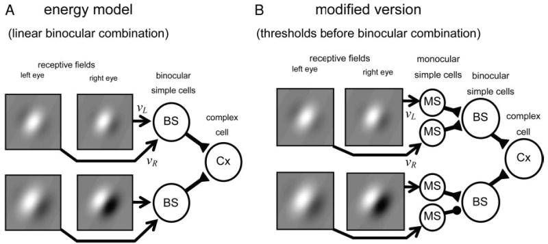
Block diagrams of the energy model (A) and our modified version (B). Grayscale plots represent receptive fields, which are shown differing in phase. Arrows show results υ_L and υ_R of a linear operation performed on image in each eye. The models do not specify physiological details of how this linear operation is calculated, so they are shown simply with arrows. Subsequently, triangles represent excitatory synapses, and disks inhibitory synapses. A: in the energy model, linear inputs from both eyes converge onto a single binocular simple cell. Each binocular simple cell computes the linear sum of its left and right inputs, and outputs the half-squared sum to the complex cell. B: possible implementation of our modified version: linear inputs from left and right eyes pass through monocular simple cells, and are thus half-wave rectified, before converging on a binocular simple cell. After this rectification, the type of synapse (excitatory/inhibitory) at the binocular simple cell has a profound influence on the type of disparity tuning observed. In B, top binocular subunit is shown receiving excitatory synaptic input from both eyes; bottom subunit is shown with one excitatory and one inhibitory synapse.

Although the energy model was originally intended as a qualitative description, its success to date suggests that it may be possible to elaborate the model so as to provide a good quantitative description of neuronal behavior. Extending the energy model requires identifying those quantitative discrepancies that have not so far been reconciled with the original structure of the model. First, the response to anticorrelated random-dot stimuli (when contrast polarity is inverted in one eye) must be accounted for. In real cells, anticorrelation inverts the disparity tuning curve and also reduces the amplitude, whereas the energy model predicts inversion only (Cumming and Parker 1997; Ohzawa et al. 1997). The amplitude reduction can be explained if we modify the energy model by incorporating threshold nonlinearities before binocular combination (Read et al. 2002). This modified version of the energy model is shown in Fig. 1B

Second, the energy model predicts that monocular stimulation in either eye should always have an excitatory effect. In this study, by making a quantitative comparison of monocular and binocular responses, we confirm that there are many cells in which input from one eye always seems to suppress the cell’s response, as previously reported by others (Ohzawa and Freeman 1986a; Prince et al. 2002a). Such behavior is inconsistent with linear binocular combination, but is predicted by our modified version (Read et al. 2002).

Third, the energy model predicts that the response to binocularly uncorrelated random-dot patterns should equal the sum of the responses to monocular random-dot patterns. In fact, it is generally much closer to their mean. It has been suggested (Prince et al. 2002b) that this is a consequence of a contrast-normalizing mechanism that tends to boost the response to monocular. We show here that the relative size of the monocular and binocular response can be explained by our modification to the energy model, without the need to invoke a normalization process.

Fourth, a key prediction of the energy model is that the shape of monocular receptive fields determines the shape of the disparity-tuned response. Although this has been verified for simple cells in the cat (Anzai et al. 1999b), the situation for complex cells is less clear because it is difficult to estimate the receptive fields of the subunits. Fortunately, the model can also be tested in the frequency domain: the Fourier power spectrum of the disparity-tuning curve should match the shape of the monocular spatial frequency-tuning curves. Preliminary testing of this prediction has indicated a conflict with the energy model prediction (Ohzawa et al. 1997; Prince et al. 2002b); however, for a number of reasons, the seriousness of this conflict is hard to assess. Prince et al. (2002b) found that their disparity tuning curves often had spatial frequency bandwidths substantially larger than those estimated from luminance gratings in other studies (de Valois et al. 1982). However, Prince et al. measured tuning for horizontal disparity, so these data are not directly comparable with selectivity for the spatial frequency (SF) of luminance gratings at the preferred orientation. Ohzawa et al. (1997) found that the frequency of the disparity-tuning curve tended to be lower than the preferred spatial frequency revealed with monocular luminance gratings in the dominant eye, apparently contradicting the energy model. However, their definition of disparity frequency could potentially obscure an underlying agreement with the energy model (see below); also, confidence intervals were not presented. Most important, neither of these studies reported measures of spatial frequency tuning in both eyes. The original energy model assumes that spatial frequency tuning is identical in the two eyes, so it is possible that the discrepancies could be attributable to binocular differences in spatial frequency tuning. If this were the case, it would be easy to extend the energy model to take account of this difference, by allowing different spatial frequency tuning between subunits, either within an eye or between eyes. The data should then agree with this generalized version of the energy model. Thus, a more complete comparison of the spatial frequency tuning and the power spectrum of the disparity tuning is necessary to test the model.

To resolve this important question, we recorded the monocular spatial frequency and orientation tuning in both eyes. This is compared with the selectivity for disparity applied to random-dot patterns along an axis orthogonal to the preferred orientation. Both comparisons systematically violate the predictions of the energy model, even after it has been generalized to allow for differences between subunits. The disparity-tuning curves show more power at lower frequencies than is possible within these models, even allowing for the presence of several subunits that may differ in position and/or spatial frequency tuning. However, once again, the results may be explained by our modified version of the energy model incorporating a threshold nonlinearity before binocular combination.

In summary, therefore, we have compared two families of models of disparity selectivity: 1) the energy model and a set of generalizations of it, all postulating linear binocular summation; and 2) our modified version incorporating threshold nonlinearities before binocular combination. For a wide range of observations, the data are quantitatively at odds with the linear model and can be accounted for by the threshold model. We conclude that adding thresholds to the energy model, before inputs from the two eyes are combined, represents a substantial step forward in our understanding of disparity selectivity in V1.

METHODS

Detailed descriptions of the general procedures have appeared elsewhere (Cumming and Parker 1999; Prince et al. 2002b). Briefly, single-unit activity was recorded from primary visual cortex (V1) of two awake macaques trained to maintain fixation while viewing stimuli for fluid reward. All protocols were approved by the Institute Animal Care and Use Committee and complied with Public Health Service policy on the humane care and use of laboratory animals.

Stimuli were generated on a Silicon Graphics Octane workstation and presented on two Eizo Flexscan F980 monitors (mean luminance 41.1 cd/m², contrast 99%, frame rate 72 Hz) viewed through a Wheatstone stereoscope, in which the monitors are viewed through mirrors positioned in front of the animal’s eyes. At the viewing distance used (89 cm) each pixel in the 1,280 × 1,024 display subtended 1.1 min arc. Antialiasing was used to render with subpixel accuracy [pixels are colored intermediate shades of gray to represent edges that only partially cover the pixel (Foley et al. 1990)]. Glass-coated platinum–iridium electrodes (FHC) were placed transdurally each day. Electrode position was controlled with a custom-made microdrive that used an ultralight stepper motor mounted directly onto the recording chamber.

The monkeys initiated a stimulus presentation by maintaining fixation on a binocularly presented spot to within ±1°. They were required to maintain fixation at this accuracy for 2.1 s to earn a fluid reward. During each such trial, 4 stimuli were presented, each lasting 420 ms, separated by 100 ms.

Stimuli

Sinusoidal luminance gratings were used to determine the minimum response field, spatial frequency, and orientation tuning of the cell. After an initial determination of the preferred spatial frequency and orientation, the monocular orientation-tuning curve in each eye was obtained using a circular patch of grating with spatial frequency reasonably close to optimal. Quantitative orientation-tuning curves usually spanned a range of 180° centered around the preferred orientation (or direction, for direction-selective cells). The spatial frequency tuning curve (SFTC) was then obtained using a large rectangular grating patch at the preferred orientation. The frequencies generally spanned 0.0625 to 16 cycles per degree (cpd) in steps of 1 octave. A pseudo-random sequence interleaving frequencies and eye of presentation was used in both cases. During monocular trials, the nonstimulated eye viewed a uniform screen of the same mean luminance.

Dynamic random-dot stereograms were composed of black and white dots, scattered at random on a gray background. The dots were usually 5 ×5 pixels (0.1° ×0.1°); for some cells, a different size was used if this enhanced the response rate. A new random stereogram was generated every frame (72 Hz). The dot density was sufficient to cover 50% of the gray background but, because the dots were allowed to overlap one another (dot location was randomly assigned with sub-pixel precision using antialiasing), the total coverage was slightly less. On average, 20% of pixels were black, 20% white, and 60% gray. Figure 2 shows an example stereogram, together with a circle indicating the size of typical V1 minimum response fields for comparison.

FIG. 2.

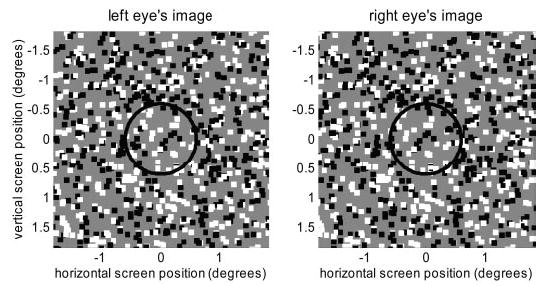
Random-dot stereogram of type used in our experiments. Dots are 0.1° ×0.1° square. Circle indicates size of typical V1 receptive field for comparison. Diameter is 1.2°, based on a subset of cells in which we obtained the one-dimensional receptive field envelope using a long luminance-modulating bar stimulus at the preferred orientation. The mean SD of Gaussians fitted to receptive field envelopes was 0.3°, and we took 4 SDs as suitable estimate of receptive field diameter.

The energy model assumes that all receptive fields feeding into a cell have the same orientation. Its predictions are therefore most easily framed in terms of disparities parallel and orthogonal to this orientation, rather than horizontal and vertical disparities. Accordingly, to facilitate testing of energy model predictions, experimental disparities were applied along the axis orthogonal to each neuron’s preferred orientation. These covered the range from −1.2° to +1.2° in the initial test for disparity selectivity, with the range −0.6° to +0.6° covered in steps of 0.1°, and steps of 0.2° outside this range. A larger range of disparities was used if necessary to ensure that there was no modulation at the extremes of the tuning curve (i.e., that the full response range had been explored). In neurons with preferred SFs >4 cpd, the central region of the curve was sampled more finely, to ensure that sampling exceeded the Nyquist limit predicted from the monocular SF tuning.

Data analysis

Data analysis such as curve fitting is greatly simplified if we can make the assumption that variance is constant across the data set. This assumption is invalid for neuronal firing rates, whose variance tends to increase in proportion with the mean (Dean 1981). However, the square root of firing rates has variance that is roughly constant, independent of the mean (Cumming and Parker 2000; Prince et al. 2002b). This variance-stabilizing transformation greatly simplifies the analysis of neuronal data. For this reason, we performed all our analysis on the square root of the recorded firing rates.

To quantify the strength of disparity tuning, we used the disparity discrimination index (DDI) introduced by Prince et al. (2002b)

$$\text{DDI}=\frac{R_{max}-R_{min}}{R_{max}-R_{min}+2{\text{RMS}}_{\text{error}}}$$ (1)

where R_max and R_min are the maximum and minimum $\sqrt{\text{firing\hspace{0.28em}rate}}$, respectively, and RMS_error is the square root of the residual variance around the mean $\sqrt{\text{firing\hspace{0.28em}rate}}$ recorded across the whole tuning curve, including the response to uncorrelated stimuli (effectively, infinite disparity). Like the more familiar binocular interaction index, (R_max−R_min)/(R_max + R_min), this is a contrast measure, except that here the difference in response between the preferred and null disparity is contrasted not with the mean response, but with the variability of the firing rate RMS_error. This means that cells in which the range in firing rates is largely the result of random fluctuations are not wrongly classified as being highly sensitive to disparity; equally, cells in which the change in firing as a function of disparity is relatively small but highly reliable are correctly described as strongly disparity-tuned. The term (R_max −R_min) in the denominator of Eq. 1 ensures that the index is bounded at 1 when the variability is small.

For most cells, monocular random-dot stimuli were also presented, in trials interleaved with binocular stimuli. Blank stimuli were also usually interleaved, where both eyes viewed a blank screen of the same mean luminance as the random-dot patterns. These were used to obtain an estimate of the spontaneous firing rate.

To allow a cell into the study, we required that binocular random dots at the optimal disparity elicit a response of at least 10 spikes/s. To proceed to quantitative analysis of the response’s shape, we further required i) ANOVA indicates a significant (P < 0.05) main effect of disparity; ii) the disparity discrimination index exceeds 0.375. The second condition removes neurons with weak but significant disparity tuning because these tend to produce noisy estimates in the quantitative analysis that follows. Including these weakly tuned neurons did not change any of the substantial results; it only increased the scatter. To subject monocular spatial frequency data to quantitative analysis, we required that i) the optimal drifting grating in that eye elicits at least 10 spikes/s; ii) ANOVA indicates a significant (P < 0.05) main effect of spatial frequency. We do not require tuning to be band-pass, and our sample included a few neurons that showed a low-pass spatial frequency tuning.

Fitting tuning curves

We summarized our tuning curves by fitting them with analytical functions. If we fitted the function directly to the mean firing rates, we would have to reduce the weight given to residuals at higher firing rates, to take account of the higher variance there. As explained above, we avoided this complication by, instead, fitting the square root of our chosen fit function to the mean of the square-root firing rates. Given that $\sqrt{\text{firing\hspace{0.28em}rate}}$ has approximately constant variance, we could then just minimize the sum of the squared residuals, without needing to weight them differently.

SFTCs were fitted with Gaussians, in either log or linear frequency space, whichever minimized the residuals. These had 4 free parameters: frequency of the peak f₀, standard deviation σ, baseline and amplitude above the baseline. The baseline was assumed to represent the spontaneous firing rate; thus, it was not allowed to be negative. The peak frequency was constrained to lie within the range of stimulus frequencies. The amplitude was not allowed to exceed twice the range of the response.

These fitted curves were used to extract a peak frequency, a low-frequency cutoff, and a high-frequency cutoff, defined as the positions where the tuning curve falls to half its maximum. Where the SFTC was fitted with a Gaussian in linear frequency, with peak at f₀ and standard deviation σ, the high and low cuts are $f_0\pm \sigma \sqrt{ln\hspace{0.17em}4}$. Where the tuning curve was fitted with a Gaussian in log frequency, with standard deviation σ in log space, the high and low cuts are $f_{0}exp(\pm \sigma \sqrt{ln\hspace{0.17em}4}).$

Disparity-tuning curves were fitted with half-wave rectified one-dimensional Gabor functions (the product of a sinusoid with an exponential; cf. APPENDIX B). The original energy model predicts a Gabor disparity-tuning curve, provided that the monocular receptive fields are narrow-band Gabor functions differing only in their position and phase. However, our main motivation for using Gabor functions is that they provide a succinct description of most experimental tuning curves (Cumming and Parker 1997; Ohzawa et al. 1990; Prince et al. 2002a). In the results section, we verify that our conclusions do not depend on the use of a fitted Gabor. One-dimensional Gabors have 6 free parameters: the spatial frequency f and phase φ of the carrier cosine, the standard deviation σ, amplitude A and center δ₀ of the Gaussian envelope, and the baseline firing rate B about which the sinusoid oscillates. Uncorrelated responses, if available, were included in the fitting; the expected response to uncorrelated stimuli is just B.δ₀ was constrained to lie within the range of stimulus disparities and the amplitude A was not allowed to exceed twice the difference between the maximum and the minimum response. The spatial frequency of the fit was not allowed to exceed half the Nyquist limit (i.e., one-quarter of the maximum spatial sampling rate of the data). Although these curves generally gave good descriptions of the tuning curves, the parameters of the fitted Gabor must be interpreted with care (see Prince et al. 2002b). When using these fits to summarize some property of the tuning curve, we therefore used appropriate measures applied to the fitted curve (illustrated by our measurement of disparity peak frequency in the next section), rather than using the parameters of the fit.

Disparity Fourier spectrum

The original energy model predicts that the disparity peak frequency, the frequency at which the disparity modulation has most power, should be the same as the preferred spatial frequency observed with monocular gratings. In making this comparison, the disparity must be applied at right angles to the cell’s preferred orientation. Most previous work using random-dot stimuli in awake animals has employed only horizontal disparities. To enable a test of the energy model prediction, all disparities in the present study were applied orthogonal to the cell’s preferred orientation (Cumming 2002). It is also important that the disparity tuning is measured with a broadband stimulus such as random dots, to ensure that the disparity tuning curve shape is not trivially determined by the stimulus. If disparity tuning were measured with a grating, for instance, the periodicity of the stimulus would guarantee a periodic response (Cumming and Parker 2000).

The disparity peak frequency is slightly different from the “disparity frequency”—a term used by two previous authors in related but distinct senses. Ohzawa et al. (1997) used a bar as the broadband stimulus to test this prediction in the anesthetized cat. They used the term “disparity frequency” to mean the carrier frequency of the Gabor fitted to the disparity tuning curve, which they then compared with the monocular spatial frequency tuning. Note, however, that this carrier frequency does not necessarily equal the disparity peak frequency. Thus their finding that the carrier frequency of fitted Gabors was systematically lower than the preferred spatial frequency in the dominant eye is not necessarily at odds with the energy model. For sufficiently narrow-band Gabor functions, the carrier frequency f and disparity peak frequency coincide (APPENDIX B), but many of the disparity tuning curves presented by Ohzawa et al. appear to be fairly broadband (e.g., their Fig. 15). In this case, the disparity peak frequency and the carrier frequency diverge. Which is higher depends on the phase of the disparity-tuning curve (APPENDIX B). The disparity-tuning curves presented by Ohzawa et al. display phases across the spectrum: thus, both situations occur. Furthermore, for Gabors that are not narrow-band, the fitted carrier frequency is often poorly constrained by data (Prince et al. 2002a; Fig. 6). For these reasons, it is not clear that the data presented by Ohzawa et al. (1997) necessarily violate the energy model.

FIG. 6.

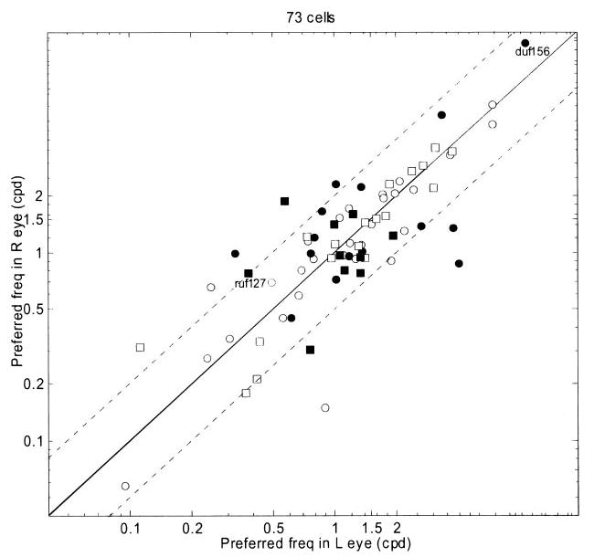
Scatter plot of preferred spatial frequency in left eye against that in right, on log axes. Preferred frequency is defined by the peak of the Gaussian fitted to the monocular tuning curve obtained with sinusoidal luminance gratings. Solid line shows identity; dotted lines mark difference in spatial frequency (SF) tuning of 1 octave. Filled symbols indicate 25 cells whose preferred frequencies in left and right eyes differed significantly (P < 0.05, resampling). Circles indicate cells from monkey Duf, squares from monkey Ruf. Cells shown in Fig. 7 are indicated. Two cells that had very low preferred spatial frequencies fall outside the range shown in the figure.

Prince et al. (2002b) used the term “disparity frequency” to refer to the peak frequency of the Fourier transform of the disparity-tuning curve after subtraction of the mean, meaning that for these authors a disparity frequency of zero is impossible by definition. The disparity frequency of Prince et al. (2002b) was designed as a way of extracting a measure of the spatial scale of disparity tuning that would work for both band-pass and low-pass tuning curves. Neither sense of disparity frequency provides the appropriate measure for comparison with monocular spatial frequency tuning: hence our use of the disparity peak frequency.

We compared two different ways of extracting the disparity peak frequency. The first was completely model-independent; here we used the response to uncorrelated stimuli as an estimate of the baseline firing rate, subtracted that from the disparity tuning curve, and took the continuous Fourier transform of the result (by trapezoidal integration). We also estimated the disparity spectrum from the Gabor function fitted to the tuning curve. When performing the fit, the Gabor function was half-wave rectified; that is, negative values of the fit function were replaced with zeros for the purpose of evaluating the residual (given that firing rates could not be lower than zero). When obtaining the disparity spectrum, we used the unrectified Gabor, and solved numerically for the peak and half-maximal points of the Fourier spectrum.

Bootstrap resampling

To interpret scientific results, it is important to have an estimate of significance, to be sure that features we observe in our data are not merely the result of the vagaries of finite sampling. Throughout this study we have used bootstrap resampling (Efron 1979) to estimate significances. Given a data set consisting of n samples of the random variable, one generates a “new data set” by randomly selecting a member of this data set n times (with replacement). This provides a convenient, nonparametric way to estimate the distribution of some function of a random variable, avoiding the normality assumptions buried in many standard statistical tests. For resampling to be reliable, n must be large. This was one motivation for presenting stimuli for relatively short periods: it provided a large number of independent samples. To increase n further, we pooled the data across all disparities (or spatial frequencies, for the grating stimuli) and resampled the residuals. For this pooling to be valid, the SD must be the same at each disparity, so, as before, we transformed each datum by taking its square root. That is, for each disparity we calculated the mean of the square root of the firing rate, and the residual difference between this mean and the square root of the firing rate on each stimulus presentation. We then pooled all these residuals into a single population. To generate a resampled datum, we picked a residual at random from this pool, added it to the mean square-root firing rate, and squared it to obtain the resampled firing rate. We also explored resampling the data for each stimulus condition separately and found that this gave closely similar results. In the few cases where the results were different, the method of resampling the residuals generally gave the wider confidence interval. Because this yields more conservative estimates for significance testing, resampling of residuals was adopted throughout. This meant that the effective n was always >80 for the SFTCs and always >200 for the disparity tuning. All quoted significances are at the 5% level.

Classification as simple or complex

Within the energy model, complex cells are viewed as being made up from the summed output of several simple cells (Eq. 3 below). Our analysis holds for both simple and complex cells and our conclusions do not depend on a classification of cells as either simple or complex. For this reason we have not treated simple and complex cells differently, and hence avoided the complications of attempting to make the classification in awake animals in the face of small eye movements.

Data set

We recorded monocular and binocular responses to random-dot stimuli in 210 neurons, at eccentricities between 2° and 10°. Of these, 180 produced a maximum firing rate of at least 10 spikes/s; 138/180 were disparity-selective. Adequate data on spatial frequency tuning were available for 101/138 disparity-selective cells, and in an additional 23 disparity-selective neurons we had data on spatial frequency tuning but not monocular responses to random dots.

The energy model and our modified version

This study represents a critical comparison of the energy model (Adelson and Bergen 1985; Fleet et al. 1996; Ohzawa 1998; Ohzawa et al. 1990; Qian 1994) and our modified version of it, introduced to explain the weaker response to anticorrelated stimuli (Read et al. 2002). In this section, we lay out the key features of both models and explain how they differ. Detailed calculations are given in the appendices.

The building blocks of all the models considered in this study are binocular subunits characterized by a receptive field in each eye, which performs a linear operation on the retinal image in that eye. The input from each eye, or υ_L υ_R, is the result of this operation (for details, see APPENDIX C, Eq. C2). The distinctive feature of the energy model is that the inputs from the two eyes are combined linearly: the response of a binocular subunit is a function of the sum (υ_L + υ_R) of the inputs from each eye separately. If this sum is negative, the binocular cell is silent because it cannot signal firing rates below zero. If this sum is positive, the energy model postulates that the binocular cell outputs the square of this sum. Thus, writing C for the output of the disparity-selective cell

$$C={[\text{Pos}(v_L+v_R)]}^2$$ (2)

where Pos denotes half-wave rectification. A complex cell is assumed to receive input from several of these half-squared linear binocular subunits, and its response is assumed to be the linear sum of its inputs

$$C=\sum _{j=1}^n{[\text{Pos}(v_{Lj}+v_{Rj})]}^2$$ (3)

This is shown schematically in Fig. 1A. Binocular subunits (“BS”) are shown receiving input from left and right eye receptive fields, which for illustration are shown with different phases. Several of these subunits feed into a single complex cell (“Cx”).

Our modified version (Read et al. 2002) differs from the energy model in postulating that inputs from the two eyes are half-wave rectified before being combined

$$C={[\text{Pos}(v_L)+\text{Pos(}{v}_R)]}^2$$ (4)

Figure 1B shows one physiologically plausible implementation of this nonlinearity. In the figure, inputs from the left and right eyes initially synapse onto monocular simple cells (“MS”), which impose an output threshold, before being combined in a binocular subunit. If the inputs are combined with an inhibitory synapse, as in the lower binocular subunit in Fig. 1B, we obtain units like

$$C={\{\text{Pos}[\text{Pos}(v_L)-\text{Pos(}{v}_R)]\}}^2$$ (5)

(the additional Pos means that the cell does not fire when suppression from the right eye exceeds excitation from the left). Once again, complex cells are constructed from the sums of several binocular units of the type given in Eq. 4 and Eq. 5 (Read et al. 2002). The distinction between the two types does not matter in the energy model: there is no need to explicitly include subtypes based on (υ_L− υ_R) as well as(υ_L + υ_R), because (υ_L −υ_R) is equivalent to (υ_L + υ_R) with a phase change of πin the right eye’s receptive field.

RESULTS

Overview

DISPARITY SELECTIVITY AND MONOCULARITY

We present evidence that some cells receive purely suppressive input from one eye. We show that this is inconsistent with the linear binocular combination of the energy model, but can be explained in our nonlinear model.

SPATIAL FREQUENCY TUNING IN THE TWO EYES

Motivated by the assumption of the original energy model that receptive fields are identical up to phase, we investigate whether there is evidence for differences in spatial frequency tuning between eyes. We find that tuning in most cells agrees well, but a minority show significant differences.

DISPARITY FREQUENCY AND SPATIAL FREQUENCY TUNING

If the assumptions of the original energy model hold, then the disparity frequency should equal the preferred spatial frequency in the dominant eye. We show that this prediction is systematically violated, and that vergence movements cannot account for the difference. However, this prediction applied only to the original energy model, which included strong constraints on the receptive field profiles in addition to linear binocular combination.

GENERALIZING THE ENERGY MODEL

We therefore generalize the energy model to allow for receptive fields with different phases, positions, and spatial frequency tuning (both across subunits, and across eyes within a subunit). We derive a constraint that even this generalized model must fulfill. We show that the data systematically violate this constraint.

THRESHOLDING BEFORE BINOCULAR COMBINATION

We finally show that our modified version of the energy model, in which a threshold precedes binocular combination, can account for the observations on disparity and spatial frequency tuning.

Disparity selectivity and monocularity

SOME CELLS RECEIVE PURELY SUPPRESSIVE INPUT FROM ONE EYE

Cells that are sensitive to binocular disparity must receive information from both eyes. It is tempting to extrapolate from this that the cells that are most sensitive to binocular disparity must be those that respond most nearly equally to input in either eye. However, previous investigators (Ohzawa and Freeman 1986b; Poggio and Fischer 1977; Prince et al. 2002b; Smith et al. 1997) have found little support for this idea. In agreement with these studies, we find no relationship between monocularity and disparity selectivity. Many cells that respond nearly equally to monocular stimulation in either eye are not disparity selective, whereas many cells that show little or no response to monocular stimulation in one of the eyes nevertheless show clear disparity tuning. Examples are shown in Fig. 3 (see also Fig. 8). The response to monocular stimulation is shown by the broken horizontal lines labeled L and R (and marked with a leftward/rightward-point arrowhead respectively: ◂and ▸). In duf096 (Fig. 3A), monocular stimulation in the left eye evokes almost no response; in duf099 (Fig.3B), it is the right eye that is silent. Yet the black dots show the cells’ responses as a function of disparity (curve = fitted Gabor); clearly both cells are selective to disparity, and so must be receiving information from both eyes. Thus, it is important to distinguish between two common uses of the term “monocular”: the classical sense, “responsive to monocular stimulation in one eye and not the other,” must not be interpreted to mean “receiving input from only one eye” (Ohzawa and Freeman 1986a, b; Smith et al. 1997).

FIG. 3.

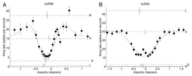
Two tuned-inhibitory cells that show evidence of an inhibitory input from one eye. Stimulation in the nondominant eye seems always to reduce firing rate: the response to monocular random dots in the nondominant eye is less than that to a blank screen, whereas the response to binocularly uncorrelated random dots is less than that to monocular random dots in the dominant eye. Disparity discrimination index = 0.61 for duf096 (A), 0.64 for duf099 (B). Filled circles (•) represent the mean firing rate as the function of disparity; the black curve is the fitted Gabor. Horizontal lines represent responses to stimuli without disparity: line labeled L and marked with leftward arrowhead ◂ indicates response to monocular random dots in left eye (R▸ : right eye); U□indicates response to binocularly uncorrelated random dots; S○indicates spontaneous rate (response to gray screen of same mean luminance). All error-bars are ± SE.

FIG. 8.

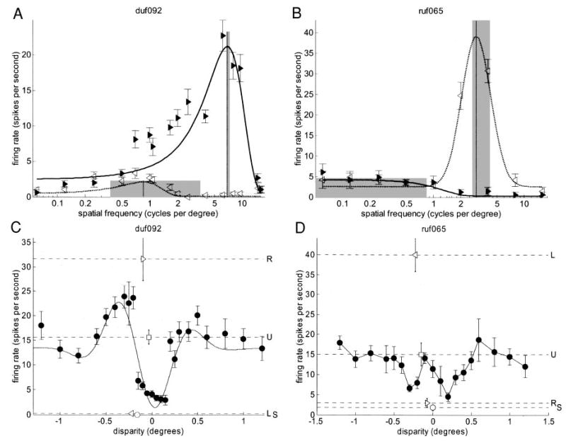
Two disparity-tuned cells (A, C: duf092; B, D: ruf065) that seem to show inhibitory influence from one eye. A, B: spatial frequency tuning (symbols as in Fig. 7); C, D: disparity tuning (symbols as in Fig. 3). For ruf065.0, disparity-tuning curve is not well fitted by a Gabor (fit explained <60% of variance); fit is therefore not shown. Disparity discrimination index = 0.58 for duf092 (C), 0.52 for ruf065 (D). For both cells, the maximum binocular response is less than the response to monocular stimulation in the dominant eye. Thus, adding dots to the nondominant eye, at any disparity, always reduces the response.

One natural way to explain the phenomenon of disparity selectivity in “monocular” neurons is to propose that the input from one eye always has a net inhibitory effect, and thus no spikes are produced by stimulation in that eye alone. In the absence of complications such as response normalization (which could adjust the response to monocular stimuli relative to binocular), such a scheme makes two predictions. First, binocularly uncorrelated dots should produce a weaker response than monocular dots in the dominant eye (because adding dots to the other eye produces net inhibition). This was the case for 86/138 disparity-tuned cells (significant in 44). Second, the monocular response in the non-dominant eye should not be significantly greater than the spontaneous response (it is rarely possible to observe a monocular response less than spontaneous, given that the latter is so frequently indistinguishable from zero); 30/138 disparity-selective neurons showed both these phenomena. In 9/30 cells, the spontaneous response was significantly greater than zero, so that if one eye had an inhibitory influence, it would be possible to observe suppression of the spontaneous response when this eye was stimulated. In 5 of these 9, the response to random-dot stimulation in the nondominant eye was smaller than the spontaneous response. The cells shown in Fig. 3 are two examples. The broken line labeled U and marked with a square (□) shows the response to uncorrelated stimuli; in both cells this is below the response to monocular stimulation in the dominant eye (i.e., adding stimulation to the nondominant eye has reduced the response). The broken line labeled S and marked with a circle (○) shows the spontaneous rate, estimated from the response to a blank screen: in both cells, the cell fires more to a blank screen than to monocular stimulation in the nondominant eye. Such examples are clearly indicative of a predominantly inhibitory input from one eye. We conclude that in many cells, stimulation in one of the eyes always has a suppressive effect.

THIS INDICATES A NONLINEARITY BEFORE BINOCULAR COMBINATION

It is important to note that this represents a substantial deviation from any model in which binocular summation is linear. By definition, a model with linear binocular summation is of the form C = f(υ _L+ υ_R), where f is an arbitrary function and υ_L and υ_R represent the inputs from left and right eyes, respectively. If f(υ_L) is never positive for any value of the input υ_L, either positive or negative (no possible stimulus in the left eye elicits a positive response), then f(υ_R) can never be positive either, and so the cell would never respond. In a linear model, if the cell responds at all, then stimulation in each eye can exert either a suppressive or an enhancing effect, depending on the stimulus. To obtain the situation where one eye always exerts a suppressive effect, we must postulate some nonlinearity before binocular combination, such as half-wave rectification followed by an inhibitory synaptic connection. This is exactly what is proposed by our modified version of the energy model. Looking at Eq. 5, C = {Pos[Pos(υ_L) − Pos(υ_R)]}², it is obvious that stimulation in the right eye always has a suppressive effect. For monocular right-eye stimulation, the response C is zero, and yet with disparate binocular stimuli, this unit is disparity-selective. Figure 4 shows simulations of two subunits described by Eq. 5. The solid line shows the disparity tuning curve. In A, the left and right receptive fields are identical, so— because input from one eye is inhibitory—the disparity tuning curve is of the tuned-inhibitory class. In B, the left and right receptive fields are 180° out of phase. When combined with the inhibitory synapse in Eq. 5, this results in tuned-excitatory disparity tuning. This demonstrates that an inhibitory synapse at binocular combination does not necessarily result in tuned-inhibitory tuning. Thus, our thresholding model explains the existence of cells that would classically be called “monocular” and yet are disparity-selective.

FIG. 4.

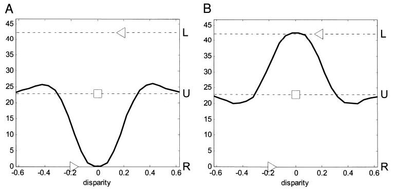
Our new model, incorporating a threshold linearity before binocular combination, can explain disparity selectivity in classically monocular cells, and cells in which the response to binocularly uncorrelated dots (U□) is close to the mean of response to monocular stimuli (L◂, R▸), rather than to its sum as predicted by energy model. Both plots show simulations for single binocular subunit receiving inhibitory input from right eye (Eq. 5); mean response over 100,000 different random-dot patterns. A: monocular receptive fields are identical, so the inhibitory synapse in Eq. 5 results in a tuned-inhibitory cell. B: left eye’s receptive field is inverse of right eye’s receptive field, so with the inhibitory synapse this results in a tuned-excitatory cell.

A THRESHOLDING NONLINEARITY CAN EXPLAIN THE RELATIVE AMPLITUDE OF MONOCULAR AND BINOCULAR RESPONSES

We now investigate the extent to which this model can account quantitatively for the relative amplitude of monocular and binocular responses. Prince et al. (2002b) observed that the response to binocularly uncorrelated dot patterns was often close to the mean of the responses to monocular stimulation in the two eyes, whereas the energy model predicts that it should be their sum. Prince et al. suggested that this could be attributable to a normalization process that lowers the response to binocular stimuli. However, our modification to the energy model already allows us to build cells in which the uncorrelated response is the mean of the 2 monocular responses, without incorporating any normalization. The horizontal lines in Fig. 4 show the response to monocular stimuli (L◃, R▹) and binocularly uncorrelated stimuli (U□). In both cases, the uncorrelated response is close to the mean of the monocular responses, demonstrating that our model can explain this phenomenon, for both tuned-excitatory and tuned-inhibitory cells.

These simulations portray something of an extreme case: in both these examples, inhibition from the suppressive eye is much stronger than excitation from the excitatory eye, so that the response to monocular stimulation in the dominant eye, M, is nearly twice the response U to uncorrelated stimuli. In fact, 2U is an upper bound for M: our model predicts that M can never exceed 2U. The energy model has a similar upper bound: it predicts that M can never exceed U. We have seen that the energy model’s upper bound is violated by most cells (86/138). We now investigate whether the upper bound predicted by our model is similarly violated. Figure 5 shows the distribution of M/U for the 138 disparity-selective cells in our data set. The vertical lines mark the upper bounds predicted by the energy model (dashed) and our model (solid). The mode of the distribution is close to M/U = 1, so over half the cells exceed the energy model upper bound. However, the distribution begins to fall off after M/U = 2, so that the upper bound predicted by our model is violated in only 23/138 cells. We used resampling to estimate the 95% confidence interval for M/U. If this interval lies entirely above 1, we can be 95% confident that the upper bound predicted by the energy is violated; this was the case for 44/138 cells (32%), shaded gray in Fig. 5. If this interval lies above 2, we can be 95% confident that the upper bound predicted by our model is violated; this was so for only 4/138 cells (3%), shaded black in Fig. 5. We conclude that almost all cells respond to monocular stimulation in the dominant eye at less than twice the rate for uncorrelated stimuli, and can therefore be accommodated within our modified model. Thus, our model can explain the observed spectrum of monocular and binocular response rates, without needing to invoke other mechanisms such as contrast normalization.

FIG. 5.

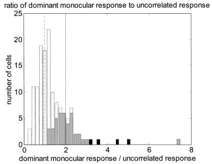
Frequency histogram for ratio of response to random-dot stimulation presented monocularly to dominant eye (M) to response to binocular uncorrelated random-dot patterns presented binocularly (U). Dashed vertical line marks M/U = 1, upper bound predicted by energy model; solid vertical line marks M/U = 2, upper bound predicted by our modified version. Shading indicates cells for which we can be 95% confident that ratio exceeds upper bound: gray shows cells where 2.5% percentile exceeded 1, black where it exceeded 2. Thus, gray + black regions indicate 44/138 cells that significantly violate upper bound predicted by energy model; black regions indicate 4/138 cells that significantly violate upper bound predicted by our model.

Spatial frequency tuning in the two eyes

The original implementation of the energy model (Ohzawa et al. 1990) assumed that all receptive fields have the same spatial frequency and orientation tuning and bandwidth. They differ only in their amplitude, their position, and phase, and even so, the position and phase disparity between left and right receptive fields of a single subunit is assumed to be the same for all subunits. These constraints on the receptive fields have been assumed by all implementations of the energy model we are aware of (e.g., Fleet et al. 1996; Lippert and Wagner 2001; Ohzawa et al. 1997; Qian 1994; Read 2002; Tsai and Victor 2003). We shall use the phrase original energy model to denote Eq. 3 with these additional constraints on the receptive fields.(Later, we shall consider a generalized energy model in which many of these constraints are relaxed.)

The available evidence suggests that these constraints are generally observed in simple cells (Anzai et al. 1999b; Ohzawa et al. 1996). In complex cells, the situation is harder to assess. Preferred orientation is observed to be closely matched between the two eyes (Bridge and Cumming 2001), supporting the view that all receptive fields share the same orientation. However, there is some evidence from the cat suggesting that there may be a population of cells in which spatial frequency differs between the two eyes (Hammond and Pomfrett 1991; Ohzawa et al. 1996). In this section, we investigate the agreement in spatial frequency tuning for our monkey data.

For 151 cells, the spatial frequency tuning to monocular drifting sinusoidal luminance gratings at the cell’s preferred orientation was probed in both eyes; 84 of these were sufficiently responsive and selective to permit fitting in both eyes. We defined the preferred spatial frequency to be the frequency at which the Gaussian fitted to the tuning curve had its peak. To ensure this is meaningful, we required the fits in each eye to explain more than 60% of the variance of the tuning curve data. Figure 6 compares the preferred spatial frequency in the two eyes for the remaining 73/84 cells. The solid line shows the identity; the dotted lines mark difference in SF tuning of 1 octave. Clearly, spatial frequency tuning is usually well matched between eyes. The correlation coefficient is 0.87 (P <10⁻⁵). Nonetheless, 25/73 cells showed a significant difference (P < 0.05, by resampling) in preferred spatial frequency between the eyes; these are colored black in Fig. 6. There was no correlation between the difference in preferred spatial frequency and the difference in peak response between the two eyes. The figure of 25 includes some cells where the difference in preferred frequency was small (but turned out to be significant because the peak positions were robust under resampling). However, for 6/25, the peak firing rates in the two eyes occurred for gratings differing in frequency by over an octave. Two examples are shown in Fig. 7. The arrowheads show the response of the cell to monocular grating stimuli as a function of the grating spatial frequency (L: ◃, R: ▸); the curves show the fit. The 95% confidence interval for the peak of the fitted function is shaded. The confidence intervals for the two eyes do not come close, indicating significant and substantial differences in spatial frequency tuning between the two eyes. About 10% of cells showed evidence of such a difference.

FIG. 7.

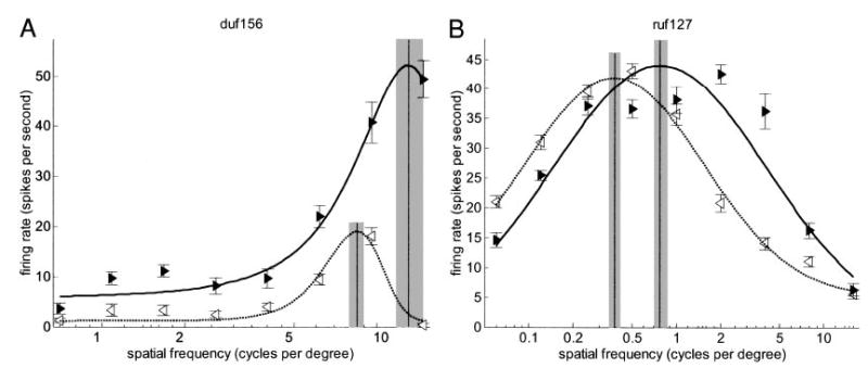
Two example cells (A: duf156; B: ruf127) that respond well to grating stimulation in either eye, but show a particularly extreme difference between spatial frequencies evoking maximum response. Triangles show mean firing rate to monocular drifting luminance gratings, as a function of spatial frequency. Error bars are ± SE. Curves are Gaussians fitted to these data; peaks are indicated with vertical lines. Shaded regions show 95% confidence interval for this peak (estimated by refitting resampled data sets). Left eye: leftward open arrowheads ◃, dotted line; right eye: rightward filled arrowheads ▸, solid line.

The selection criteria applied in obtaining Fig. 6 exclude an interesting class of cells in which the response in the nondominant eye was very weak, but was maximal at those frequencies that produced the weakest responses in the dominant eye. Two examples are illustrated in Fig. 8, A and B. On the face of it, these cells show a severe mismatch in spatial frequency tuning, with the nondominant eye being tuned to frequencies an order of magnitude lower than the dominant eye. However, we believe a more plausible explanation is that the spatial structure of the receptive fields is really similar in the two eyes (as in the vast majority of cells, Fig. 6), but that the nondominant eye exerts a suppressive effect. This interpretation is supported by the experiments with random-dot patterns. Both these cells are disparity-selective, but also show virtually no response to random dots in the nondominant eye (Fig. 8, C and D). Thus, such cases are further evidence for purely inhibitory input from one eye.

Disparity frequency and spatial frequency tuning

We now turn to possibly the most important prediction of the energy model: the shape of monocular receptive fields determines the shape of the disparity-tuned response (Anzai et al. 1999b; Ohzawa et al. 1997). Because most cells do indeed show similar spatial frequency and orientation tuning in the two eyes, we shall assume in this section that the assumptions of the original energy model hold true. Then, the original energy model predicts that the disparity-tuning curve is simply the cross-correlation of the receptive fields in the left and right eyes.

For simple cells, which are single binocular subunits (Eq. 2), this prediction can be tested directly. For complex cells, which represent the sum of several binocular subunits (Eq. 3), the disparity tuning curve is predicted to be the sum of the cross-correlations of the receptive fields in the component subunits. This makes the prediction hard to test in complex cells because it is difficult to obtain the receptive fields of the component subunits experimentally. Fortunately, provided all subunit receptive fields have the same preferred orientation, the comparison can be made without a direct measurement of receptive field profile. We simply need to obtain 1) the cell’s response to binocular random-dot patterns as a function of disparity along an axis orthogonal to this preferred orientation, and 2) the cell’s response to monocular sinusoidal gratings oriented parallel to this preferred orientation, as a function of spatial frequency. The energy model predicts that the shape of the Fourier amplitude spectrum of the disparity tuning curve measured in 1) will be given by the monocular spatial frequency tuning curves measured in 2). In particular, their peaks should coincide: that is, the disparity peak frequency, defined as the position of the peak in the Fourier amplitude spectrum, should be the preferred spatial frequency of the cell. This key prediction of the original energy model, which depends critically on its linear properties, holds for both simple and complex cells. Previous work (Ohzawa et al. 1997; Prince et al. 2002b) has suggested that this prediction is not fulfilled, but, as discussed above, these studies leave open a number of possible ways in which the data could be reconciled with the energy model. We carried out a detailed comparison, using bootstrap resampling to estimate the significance of any discrepancy.

Figure 9 shows the comparison for 3 neurons, illustrating the common patterns observed. The left-hand column shows the disparity tuning curves. On the right, the Fourier amplitude spectrum of the disparity-modulated component is compared with the spatial frequency tuning in the dominant eye. For both these quantities, two estimates are shown: one from the raw data and one from the fitted function. The raw SFTCs are shown with filled circles (•) in the plots on the right, whereas the fits are drawn with the black curve. The disparity-modulated component can be estimated from the raw data by sub- tracting the mean response to uncorrelated stimuli (horizontal line labeled with the letter U and the symbol □in the left-hand plots) from the mean response of the cell to random-dot stereograms at different disparities [filled circles (•) in the plots on the left]. The Fourier spectrum of this is shown on the right with a dotted gray line [“FT-DMC (data)” in the legend]. Alternatively, the disparity-modulated component can be obtained from the fitted Gabor (solid curve in the left-hand plots). The Fourier spectrum of this is shown on the right with a dashed gray line [“FT-DMC (fit)”].

FIG. 9.

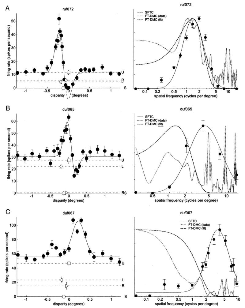
Comparing disparity and spatial frequency tuning. Left: disparity-tuning curves (symbols as in Fig. 3). For ruf072 (A), dashed curve shows unrectified Gabor, which dips below zero. Right: Fourier transform of disparity-modulated component of disparity-tuning curve (FT-DMC; gray) compared with spatial frequency tuning curve (SFTC) in dominant eye (SFTC; black), scaled to same peak value. Black dots: mean firing rate as function of spatial frequency; black curve: log-Gaussian fitted to these data. Dotted gray line [“FT-DMC (data)”]: Fourier amplitude spectrum of raw disparity-tuning curve minus mean response to uncorrelated stimuli. Dashed gray line [“FT-DMC (fit)”]: Fourier amplitude spectrum of fitted Gabor minus fitted baseline. A: ruf072: FT-DMC resembles SFTC. B: duf065: FT-DMC appears shifted toward lower frequencies than SFTC. C: duf067: FT-DMC is low-pass, SFTC is band-pass.

In a few cases (Fig. 9A) the Fourier transform of the disparity-modulated component (FT-DMC) did closely resemble the SFTC, but for the majority of cases there were substantial discrepancies, of two types. First, the peak of the FT-DMC was often at a lower frequency than the peak of the SFTC (Fig. 9B). Second, the FT-DMC was often close to low-pass in form, despite a clear band-pass SFTC (Fig. 9C).

We had 105 disparity-selective neurons that were sufficiently responsive to gratings in the dominant eye, selective for spatial frequency, and adequately described (>60% variance explained) by the Gaussian fit. To avoid making the assumption that all disparity tuning curves were well described by Gabors, we first used a model-independent estimate of the disparity peak frequency, using the response to uncorrelated stimuli as an estimate of the baseline of the disparity tuning curve, and taking the continuous Fourier transform of the raw data. We compared this estimate of disparity peak frequency with the SFTC peak frequency of the Gaussian fit, for the 105/112 cells in which the response to uncorrelated stimuli was available and in which the Gaussian fitted to the SFTC explained >60% of the variance. The disparity peak frequency was less than the SFTC peak frequency in 84/105 of cells [P <10⁻⁹ under the null hypothesis that the estimated disparity peak frequency is as likely to be above the SFTC peak frequency as below it (binomial distribution)]. The frequency difference was individually significant in 43/84 cells.

This model-independent method of extracting the disparity peak frequency has two disadvantages. First, in about 10% of cells, the disparity tuning curve appeared to be truncated by the lower limit of 0 spikes/s. These cells may represent an energy model unit followed by an output threshold. It is possible that the discrepancy between the disparity peak frequency obtained from the raw data, and the SFTC peak frequency, may reflect distortions introduced into the Fourier spectrum by the threshold. For these cells, a better estimate of the underlying response may be gained from the unrectified Gabor corresponding to the half-wave rectified Gabor fitted to the data (shown in Fig. 9A). Second, because the Fourier spectra of raw data are usually noisy and multimodal, it is hard to extract measures of bandwidth. Again, this is solved by using the fitted Gabor.

For those 99 cells in which the Gabor fitted to the disparity tuning curve explained >60% of the variance, we therefore repeated the analysis using the estimate of disparity peak frequency derived from the fit. The results are shown in Fig. 10A, which plots the disparity peak frequency against the preferred spatial frequency in the dominant eye, both derived from the fitted functions. The solid line marks the identity line; according to the energy model, all points should lie on this line. In fact, the SFTC peak frequency was greater than the disparity peak frequency in 80/99 cells (P < 10⁻⁹, binomial), and the difference was significant in 51/80 individual cells (resampling; these are the filled symbols in Fig. 10A). Thus, we obtain very similar results whether we use the fitted Gabor or the raw disparity tuning curve.

FIG. 10.

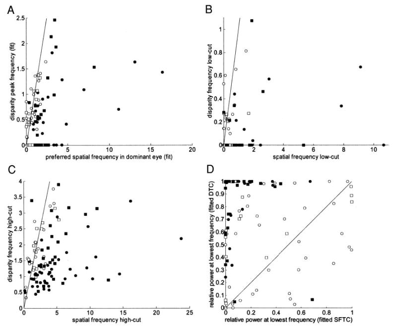
These 4 panels compare the Fourier spectrum of the disparity tuning curve (FT-DMC), after subtraction of the fitted baseline, with the grating spatial frequency tuning in the dominant eye. In each case, the identity line is marked, and filled symbols show cells where properties of disparity tuning curve differed significantly from those obtained with gratings (P < 5%, resampling). Circles indicate cells from monkey Duf, squares from Ruf. All quantities were estimated from fits to data (99 cells). A: frequency at which Fourier spectrum peaks. B, C: low cut and high cut, i.e., frequencies on either side of peak at which fitted spectrum falls to half its maximum value. In A–C, one cell falls outside range of axes; in each case its FT-DMC values were higher than SFTC values, but this difference was not significant. D: relative power at lowest frequency tested monocularly (i.e., power at this lowest frequency, normalized by the power at the peak of the frequency spectrum).

We also examined the high and low cutoff frequencies of the fitted functions. Figure 10, B and C plot the cutoff frequencies for the disparity tuning curve against those for the SFTCs. Again, the energy model predicts that all points should lie on the identity line (marked with the solid line). In fact, the low cuts differed significantly in 43/99 of cells, whereas the high cuts differed in 67/99 (filled symbols). Once again these significant differences nearly all reflect relatively more power at low frequencies in the FT-DMC than in the SFTC.

In many cases, there is so little attenuation of the FT-DMC at low frequencies that the low-cut frequency is not defined (plotted as a low cut of zero). The discrepancy in the response at very low frequencies is made clearer in Fig. 10D, which compares the relative power at the lowest frequency tested monocularly. In 77/99 cells, the FT-DMC contains more power at these low frequencies than the SFTC (P <10⁻⁶, binomial). In 45/77 cases, this difference is significant (filled symbols). In many cases, the disparity tuning curve is close to Gaussian in form (relative power = 1; i.e., no attenuation at low frequencies). That this occurs in the presence of a band-pass SFTC is a dramatic deviation from the energy model. The band-pass SFTC implies that the receptive fields of the subunits contain both “on” and “off” subregions. At a disparity equal to the separation of the “on” and “off” regions, the contributions from the left and right eyes should be negatively correlated, producing a response that is smaller than the response to uncorrelated dots. These suppressive side lobes in the disparity-tuning curves are often not found. Prince et al. (2002b) also noted that many disparity-tuning curves were Gaussian in form. However, those data were not clearly at odds with the energy model for two reasons. First, disparity was applied horizontally, regardless of receptive field orientation, so it remained possible that suppressive side lobes would have emerged if disparity had been applied orthogonally to the preferred orientation. Second, their data on spatial frequency tuning were not generally sufficient to exclude the possibility of a substantial low-pass component in the monocular SFTC. The present data eliminate both of these difficulties, and clearly indicate a need for more complex processing than the original energy model can provide.

VERGENCE EYE MOVEMENTS ARE UNLIKELY TO EXPLAIN THE MISMATCH

One possible explanation of the mismatch between disparity tuning and spatial frequency tuning is that the monkeys may be making small vergence movements. This would have the effect of introducing jitter into the disparity of each stimulus. Effectively, we would be summing several disparity tuning curves of the form predicted by the energy model, each with a random disparity offset. This tends to smear out the sidelobes, shifting the peak of the disparity power spectrum to lower frequencies. This process is illustrated in Fig. 11. Consider an energy-model binocular subunit, whose receptive fields in both eyes are identical, with no position disparity, both having the profile shown in Fig. 11A. The thin line in Fig. 11B shows the disparity tuning curve that would be obtained for this subunit in the absence of vergence movements. Now suppose the monkey makes random vergence movements, so that the disparity of his actual fixation point relative to the fixation target at any moment is a Gaussian centered on zero. This means that the disparity-tuning curve actually measured is the true curve convolved with this Gaussian. The result is shown with the thick line in Fig. 11B. Figure 11C shows the effect on the Fourier amplitude spectrum of the disparity-modulated component. The thin line shows the power spectrum for the original tuning curve, and the thick line for the observed version contaminated by vergence. The vergence has had two effects: it has shifted the peak of the disparity power spectrum toward DC, and it has greatly reduced the amplitude. For clarity, therefore, the broken line shows the observed disparity power spectrum scaled up to the same amplitude as the uncontaminated one. The same effect would be obtained if the neuron being recorded from represented the sum of several subunits that differed in their position disparities.

FIG. 11.

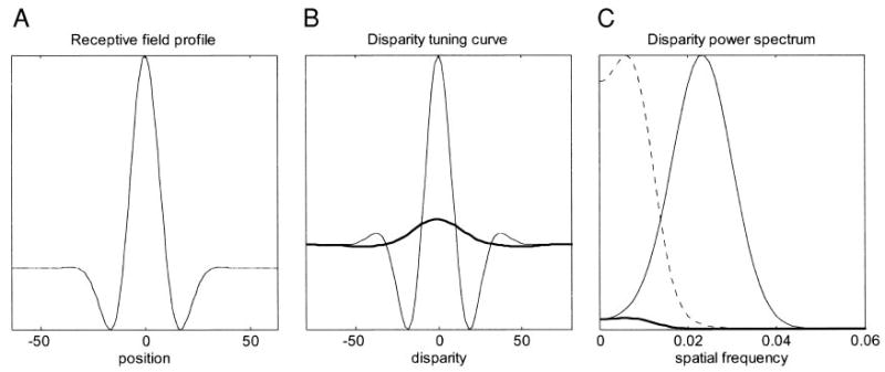
Effect of vergence eye movements, or several subunits with different position disparities. A: receptive field profile: a Gabor function yielding a spatial frequency bandwidth of 1.5 octaves. B: thin line shows autocorrelogram of this receptive field, which is the disparity-tuning curve predicted by the energy model (Eq. C1). Heavy line shows the disparity-tuning curve that would be obtained by combining output of many such subunits, as in Eq. D5, each with the receptive field profile shown but differing in position disparity. To obtain the curve shown here, 1,000 subunits were used, with random-position disparity drawn from a Gaussian with mean zero and SD equal to half the spatial period of the Gabor carrier. This simulates random jitter in monkey’s vergence. C: compares Fourier power spectrum for a single subunit (thin line) and for 1,000 subunits (heavy line). Dotted line shows 1,000 subunit result scaled up to same peak. For a single subunit, the disparity power spectrum peaks near the frequency of the Gabor carrier. Adding more subunits with a scatter in position disparity removed power at high frequencies, shifting the peak to lower frequency.

Either of these possibilities might explain why, in 80/99 cells, the peak of the disparity power spectrum is at a lower frequency than the preferred spatial frequency obtained with gratings. To estimate the vergence jitter that would be necessary to achieve this, we assume that the underlying disparity-tuning curve is a Gabor with disparity peak frequency equal to the preferred spatial frequency in the dominant eye, and that the Gabor function fitted to the observed disparity-tuning curve represents this underlying disparity tuning curve convolved with a Gaussian distribution of vergence. In over half the cells (48/80), the amount of vergence jitter needed to bring about the requisite shift in frequency is larger than the SD of vergence reported by the scleral search coils, even though search coils clearly overestimate variability in vergence (Read and Cumming 2003). It therefore seems unlikely that the animal’s vergence jitter is large enough to explain the mismatch in peak frequency in most cells.

Generalizing the energy model

It remains possible that combinations of subunits with different position disparities might be responsible for the lower disparity frequency. However, even if this is the case, the energy model places an upper limit on the power at any frequency. This can be appreciated by inspecting Fig. 11. The multiple subunits have shifted the peak toward lower frequencies, but they have done this by removing power at high frequencies rather than by adding power at any frequency. If multiple subunits are responsible for the mismatch between disparity peak frequency and preferred spatial frequency, the overall power in the disparity tuning should be greatly reduced. We therefore generalized the energy model to examine the possibility that such scatter in positions could explain our data.

In the original formulation of the energy model (Ohzawa et al. 1990), all binocular subunits were assumed to have the same phase disparity, position disparity, spatial frequency, and orientation tuning. We now allow an arbitrary number of subunits, with different phases, positions, and spatial frequency tuning (both across subunits and across eyes within a subunit), including monocular subunits and binocular subunits that are not tuned to disparity. We shall, however, continue to assume that all receptive fields have the same orientation, and the same profile parallel to this orientation (see APPENDIX E). With this much weaker set of constraints on the receptive fields, it is no longer true that the disparity Fourier spectrum must have the same shape as the spatial frequency tuning. However, it can be shown (APPENDIX E; Eq. E9) that the disparity power spectrum, ${\left|\tilde{D}(f)\right|}^2,$ and the product of the monocular spatial frequency tuning curves, L_SF(f)R_SF(f) must still satisfy the following inequality, for every spatial frequency f:

$$\frac{L_{\text{SF}}(f)R_{\text{SF}}(f)}{L_{\text{ASF}}{R}_{\text{ASF}}}\ge \frac{{\left|\tilde{D}(f)\right|}^2}{U^2}$$ (6)

The monocular spatial frequency tuning curves have been normalized to unit area by dividing by the area under each curve, L_ASF and R_ASF. The disparity power spectrum has been normalized by dividing by the squared response to uncorrelated random-dot stereograms U². This has the advantage of canceling out any differences in the overall response to sine gratings and to random-dot stimuli (e.g., because random dots have less contrast power in the cell’s spatial band-pass, or because of stimulus-dependent change in width- or end-stopping). Because such effects apply equally to disparate and uncorrelated stereograms, they would cancel out in Eq. 6. For the original energy model, Eq. 6 holds with an equals sign.

This inequality allows us to detect whether the lower disparity frequency can be explained by the presence of multiple subunits with different positions, as in Fig. 11. Then, the shift in the peak frequency would be achieved not by boosting the disparity power at low frequencies, but only by removing power at high frequencies. This would substantially weaken the disparity modulation (cf. Fig. 11B), so that the inequality Eq. 6 would be satisfied. If the inequality is violated, then multiple subunits are not a sufficient explanation.

The same generalization allows for differences in spatial frequency tuning between eyes. Our analysis in the previous section [like that of Ohzawa et al. (1997)] considered only the dominant eye, and assumed that the SFTC in the nondominant eye differed only by a scaling of response magnitude. Yet our results (Figs. 6 and 7) show that there is a significant minority of cells in which spatial frequency tuning differs between eyes. The inequality of Eq. 6, which includes terms for the spatial frequency tuning in each eye, holds for the generalized energy model even in this case.

The top row of Fig. 12 (A–C) examines Eq. 6 for one cell, ruf030, which satisfied the energy model prediction reasonably well. Figure 12A shows the SF tuning in the two eyes together with the fitted functions; Fig. 12B shows the disparity-tuning curve, with the 95% confidence interval at each disparity shaded. Figure 12C compares the fitted grating curve L_SF(f)R_SF(f)/L_ASFR_ASF (black) and disparity spectrum ${\left|\tilde{D}(f)\right|}^2/U^2$ (gray). The disparity peak frequency is at 0.82, whereas that of the grating curve is at 0.24. This difference was significant, so the data are incompatible with the simplest form of the energy model. Because the disparity peak frequency is, atypically, higher than the SFTC peak frequency, this cannot be explained by vergence eye movements. However, because the inequality of Eq. 6 is not significantly violated at most frequencies, the data are fairly compatible with our generalized version of the energy model, incorporating many subunits with different spatial frequency and/or disparity tuning. Note that the odd-symmetric disparity tuning in this cell cannot arise simply from a phase disparity of π/2 between receptive fields whose properties are otherwise identical, as originally envisaged by Ohzawa et al. (1990), because this would require the normalized curves in Fig. 12C to peak at the same frequency. One possibility is that this cell receives input from one tuned-excitatory subunit with a position disparity of 0° and one tuned-inhibitory subunit with a position disparity of 0.5°, resulting in the odd-symmetric curve. Such a scheme is allowed within this generalized version of the energy model, but is nevertheless very different from previous explanations of odd-symmetric disparity tuning (DeAngelis et al. 1991; Ohzawa et al. 1990). Some properties of such a model are discussed in Read et al. (2002).

FIG. 12.

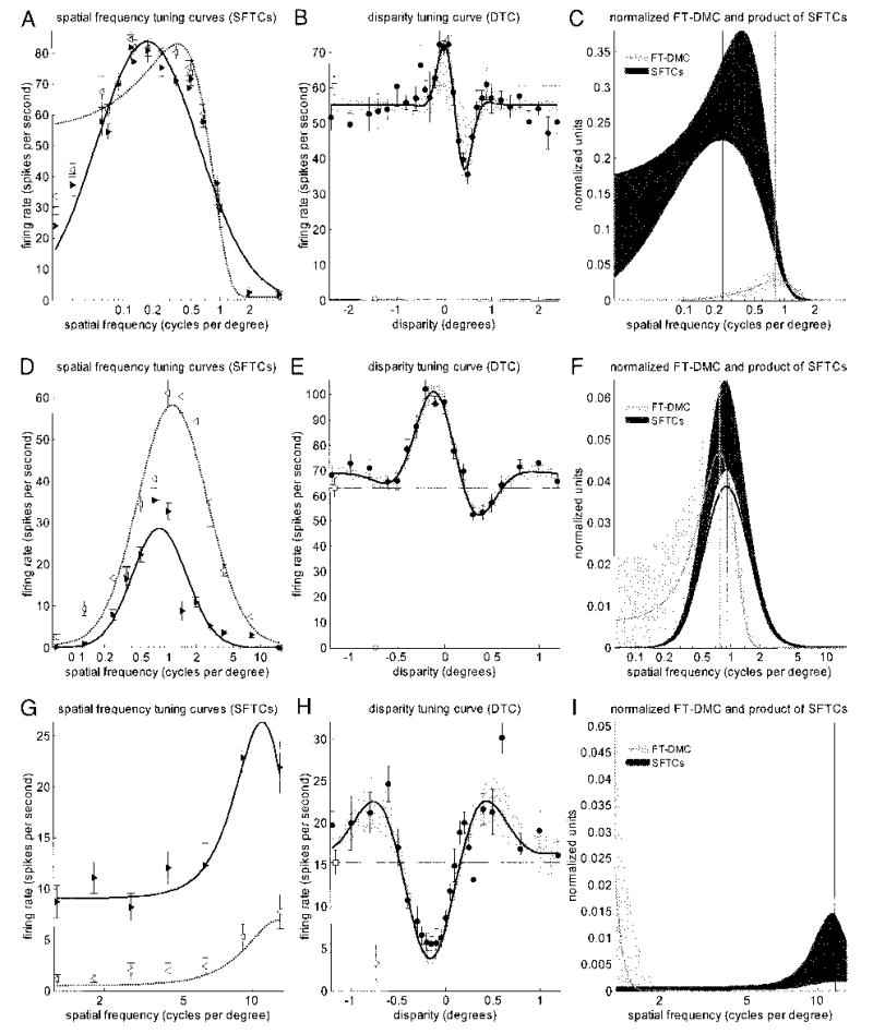
Comparison of spatial frequency and disparity tuning for 3 example cells. Left column (A, D, G): monocular spatial frequency tuning curves (left eye: leftward open arrowheads ◃, dotted line; right eye: rightward filled arrowheads ▸, solid line). Middle column (B, E, H): filled circles (•) show disparity tuning curve. Curve shows fitted Gabor; shaded region shows 95% confidence interval for fitted functions. Broken horizontal lines show response to uncorrelated stimuli (upper line, □) and to blank screen (lower line, ○). In each case, symbols and error bars show mean ± SE. Right column (C, F, I): black line shows product of left and right spatial frequency tuning curves, normalized by area underneath each. Gray line shows Fourier power spectrum of disparity tuning curve minus fitted baseline, normalized by square of fitted baseline. Shaded regions around curves show 95% confidence intervals, estimated by fitting resampled data. Position of peak of each curve is marked with vertical lines. Generalized energy model predicts that gray curve should always lie below black curve (Eq. 6). Top row (A, B, C): ruf030: a cell that is mostly consistent with the energy model. At low frequencies, normalized power spectrum of the disparity tuning curve is not significantly greater than the product of the monocular SFTCs, in accordance with the generalized energy model. (At high frequencies, the inequality is in fact violated, so even this cell may not be entirely compatible with the energy model.) Middle row (D, E, F): ruf139: the cell that violates a generalized energy model. At low frequencies, the normalized disparity spectrum (gray region in F) is significantly higher than the normalized product of the SFTCs (dark region in F), in violation of Eq. 6. Note that an analysis only of the peak frequency of these two curves would not have revealed this discrepancy. Bottom row (G, H, I): duf096: another cell that violates the generalized energy model. SFTCs peak at high frequencies: over 10 cpd. In contrast, the disparity tuning curve has most power at DC, and no power at all at 10 cpd.

More typical results are shown in the bottom two rows of Fig. 12. The cell in Fig. 12F is an example where the peak frequencies (marked by vertical lines) are close, so that an analysis only of the peak frequency would conclude that it is consistent with the energy model. However, over a range of low frequencies, the scaled disparity power spectrum is significantly higher than is possible under the energy model. The SFTCs indicate no response to a DC stimulus, so according to the energy model the disparity-tuning curve should have no DC component. In the energy model, the disparity-tuning curve of a complex cell is the sum of the disparity-tuning curves for the individual subunits. This cannot produce a curve with a DC component that is absent from all the subunits. The bottom row of Fig. 12 (G–I) shows another example that severely violates the inequality. The SFTCs peak at high frequencies: over 10 cpd. In contrast, the disparity-tuning curve has most power at DC, and no power at all at 10 cpd. Once again, the power at DC is far beyond what could be accounted for by multiple subunits. The 3 example cells shown in Fig. 9 also violate the inequality.

To quantify the results across the entire data set, we used the difference

$$\mathrm{\Delta }=\frac{L_{\text{SF}}(f)R_{\text{SF}}(f)}{L_{\text{ASF}}{R}_{\text{ASF}}}-\frac{{\left|\tilde{D}(f)\right|}^2}{U^2}$$ (7)

This is the difference between the black curve and the gray curve in the right-hand column of Fig. 12 (C, F, I). The energy model, generalized to include many subunits, predicts that Δshould be positive or zero for all frequencies (Eq. 6); that is, the black curve above the gray curve in Fig. 12, C, F, and I. Using the functions fitted to the disparity and SF tuning, we evaluated Δat a range of frequencies. We used resampling to estimate the 95% percentile of this difference; if this percentile is negative, we can reject the inequality of Eq. 6 with 95% confidence.

We had 83 disparity-tuned cells for which SFTCs were available in both eyes, and for which all 3 fitted functions explained more than 60% of the variance. For frequencies lower than the peak of the product of the SFTCs, the hypothesis Δ ≥ 0 could confidently be rejected for over half of the cells. The significance of the rejection in individual cells was often very high. At a frequency of 0.01 cpd, the hypothesis could be rejected with 95% confidence for 47/83 cells, and with better than 99.99% confidence for 13/83 cells. Figure 13 shows how the proportion of cells for which the energy model can be rejected (i.e., Δ significantly less than zero) varies depending on the frequency at which Δ is evaluated. To make a meaningful definition of “low frequencies” across a population with differing SF tuning, we express frequencies relative to the peak. This shows clearly that, whereas at high frequencies most cells appear consistent with the generalized energy model, significant discrepancies emerge as we move toward lower frequencies. Thus, although a more general version of the energy model can explain the differences in the peak frequencies previously reported (Ohzawa et al. 1997; Prince et al. 2002b), the absolute power at low frequencies in the FT-DMC still allows us to reject the energy model in over half the cells. Note that this analysis also demonstrates that no amount of vergence variability could explain the data in these cells. If the vergence variability was large enough to account for the necessary shift in disparity peak frequency, it would have reduced the amplitude of disparity tuning below that observed. We conclude that the disparity-selective responses of many V1 neurons are not compatible with the energy model, even after it has been generalized to include multiple subunits with different SF and disparity tuning.

FIG. 13.

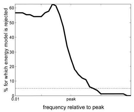
At low frequencies, over half of cells are incompatible with energy model. The energy model predicts that Δ (Eq. 7) is nonnegative at every frequency. For each of 83 cells, we evaluated Δ at a range of frequencies. The solid curve shows the percentage of cells for which the energy model hypothesis that Δ is nonnegative could be rejected at the 5% level (dotted line). For low frequencies, the energy model can be rejected for around half the cells. We used Gaussian/Gabor functions fitted to the data. SFTCs were assumed to be zero outside the range of frequencies tested (even though the fitted curve does not necessarily fall to zero, given that a baseline was included in Gaussian fit). To make a meaningful definition of “low frequencies” across a population with differing SF tuning, we evaluated Δ at 32 frequencies, of which the lowest was always 0.01 cpd, whereas the 16th was the peak of the product of SFTCs (marked “peak” in figure). Other frequencies were scaled at equal increments in ln (frequency). The graph shows that, at frequencies below the SFTC peak, the energy model can usually be rejected, because the disparity tuning contains more power than expected on the basis of SF tuning (cf. Figs. 9 and 10).

THE POSSIBLE SOURCES OF ERROR CANNOT EXPLAIN THE MISMATCH

Spontaneous firing rates

An overestimate of the area under the SFTC would yield excessively small values for the normalized product of SFTCs, which might cause erroneous rejection of the energy model. This could occur if a substantial spontaneous firing rate was added to the response resulting from receptive field structure. However, the observed spontaneous rates were almost always very low. For 211 of the 252 cells, blank stimuli, consisting of a uniform gray screen at the mean luminance of the random dots, were interleaved with the disparate random dots. The mean blank response, averaged over these 211 cells, was 2.1 spikes/s. The mean response exceeded 10 Hz in only 13/211 cells.

Orientation misalignment

Care was taken to ensure that disparity tuning and SF tuning were measured along the same axis, but of course this may not have been exactly orthogonal to the receptive field orientation. Such a misalignment will mean that Eq. 6 does not hold in general, and the effects will depend on the monocular receptive field. For Gabor-receptive fields that are longer in the direction parallel to the carrier Gabor than in the direction orthogonal to it, such misalignment always moves the peak of the product of the monocular SFTC to lower frequencies, while having less effect on the disparity frequency (APPENDIX F). Thus, for these respective fields, the disparity frequency should be if anything higher than the frequency of the peak of the product of monocular SFTCs, the opposite of the observed pattern. Thus, it seems unlikely that our results reflect any artifact of this kind.

Thresholding before binocular combination can explain the mismatch

It is therefore clear that the energy model, either in its original form or as generalized here, cannot account for the data. More elaborate extensions of the energy model are needed to reconcile it with experimental observations. We previously (Read et al. 2002) extended the energy model by adding thresholds before binocular combination (Eq. 4). We introduced this modification to explain the reduced response of V1 neurons to binocularly anticorrelated stimuli. We have already seen that this same modification also explains the phenomenon of disparity selectivity in classically “monocular” cells. We now show that the same modification also explains the existence of low-pass disparity tuning curves in cells that have band-pass SF tuning.

Figure 14 compares disparity and SF tuning for the generalized energy model (top row, A–C) and for our modified version with two different sets of parameters (bottom two rows: D–F, G–I). The layout is the same as in Fig. 12: the left-hand column shows the SFTCs obtained with grating stimuli, the middle column shows the disparity tuning curve and the response to uncorrelated random-dot patterns, whereas the right-hand column compares the normalized Fourier power spectrum of the disparity-modulated component (FT-DMC, gray curve) and the product of the normalized SFTCs (black curve). We have chosen an example in which the SF tuning is different in the two eyes: the left eye is tuned to a SF of 2.5 cpd, and the right eye to 3.5 cpd.

FIG. 14.

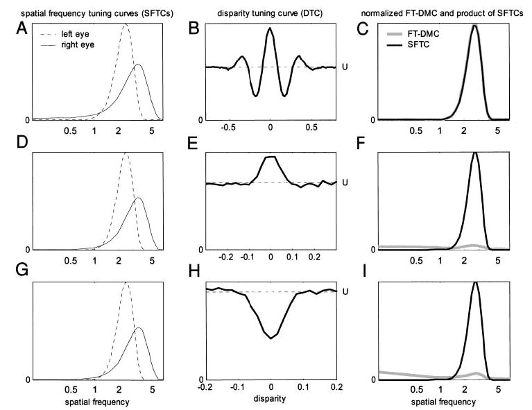
Comparison of simulated spatial frequency and disparity tuning for 3 model cells. Left column (A, D, G): monocular SFTCs (Left eye: dotted line; Right eye: solid line). Middle column (B, E, H): disparity-tuning curve (black curve) and response to uncorrelated stimuli (broken line, U). Note that horizontal axis has different scale in B, E, and H. Right column (C, F, I): black line shows product of left and right SFTCs, normalized by area underneath each. Gray line shows Fourier power spectrum of disparity tuning curve about baseline, normalized by square of response to uncorrelated stimuli. Receptive fields are two-dimensional Gabor functions, tuned to 2.5 cpd (left eye) and 3.5 cpd (right eye). Top row (A, B, C): energy model binocular subunit, C = [Pos(υ_L+υ_R)]². Middle row (D, E, F): same binocular subunit modified to include high threshold before binocular combination: C = [Θ(υ_L) + Θ(υ_R)] ², where Θ represents a threshold function: Θ_(x) = (x − Θ) if x exceeds the threshold θ, and 0 otherwise. Value of threshold θ was set so high that only 5% of monocular random-dot patterns evoked a response. Bottom row (G, H, I): sum of 2 binocular subunits including same threshold nonlinearity as above, plus an inhibitory synapse: C = [Pos{Θ(υ_L) − Θ(υ_R)}]² + [Pos{Θ(υ_R) − Θ(υ_L)}]². A pair of complementary subunits is chosen to give a monocular response in both eyes (clearly, a single inhibitory subunit would violate the inequality even more dramatically, since the product of the spatial frequency-tuning curves would be zero). In each case, the disparity-tuning curve represents the mean response to 100,000 different random-dot patterns.

In the top row, we show results for a single binocular subunit, combining left- and right-eye inputs linearly in accordance with the energy model. Because there is only a single subunit, the normalized FT-DMC is identical to the product of the normalized SFTCs (Fig. 14C) [i.e., Eq. 6 holds with an equals sign (cf. APPENDIX E)]. The inequality is thus satisfied.

The middle row, Figure 14, D–F, shows the same quantities for a binocular subunit in which the inputs from left and right eyes have been passed through a high-threshold nonlinearity before being summed and squared. This has completely removed the inhibitory side lobes that were present for the energy model subunit in Fig. 14B, resulting in a low-pass disparity power spectrum. The inequality of Eq. 6 is violated, just as in real data.

The bottom row, Figure 14, G–I, shows a similar nonlinear model, this time with an inhibitory synapse resulting in a tuned-inhibitory-type disparity-tuning curve (given that the left and right receptive fields are in phase). For a single subunit, the SFTC in the inhibitory eye would be zero, so the product of the SFTCs would be zero and the inequality would be severely violated. Because it was rare for a completely silent SFTC to be recorded in one eye, this would be a rather extreme example. Instead, we make our model cell the sum of 2 binocular subunits, with identical left and right receptive fields. In the first subunit, the left eye is excitatory and the right eye inhibitory; in the second subunit, it is the other way around. Thus, the response observed for grating stimuli in the left eye is entirely attributable to the first subunit, whereas the response to gratings in the right eye is entirely attributable to the second subunit, although both subunits contribute to the disparity-tuning curve. Thus, in our modified version of the energy model, power present in the disparity-tuning curve does not necessarily show up in the SFTC. This is why the disparity power spectrum for this model cell rises well above the product of the SFTCs at low frequencies (Fig. 14I). This behavior is incompatible with the generalized energy model, but is commonly observed experimentally (Fig. 12, F and I). We conclude that our modified version of the energy model provides a better match to the data.

DISCUSSION

The energy model of binocular complex cells has been successful in qualitatively capturing several aspects of their function. However, several quantitative predictions are not borne out by experimental data. In this study, we document two such discrepancies. We demonstrate that in each case, the agreement with data is better if we modify the energy model by adding threshold nonlinearities before binocular combination.

The first problem for the energy model is that there are many cells in which input from one eye appears to be predominantly inhibitory. The energy model is linear up to binocular combination, and this means that inputs from each eye can be both positive or negative, depending on the particular stimulus. For example, if a receptive field in one eye consists of a single on region, then a random-dot pattern in which mainly white dots happen to fall on the receptive field will elicit an excitatory response from this eye, whereas a pattern in which the receptive field is covered predominantly with black dots will elicit an inhibitory effect. Thus we cannot classify this eye as being “excitatory” or “inhibitory.” However, previous workers have noted cases where one eye appears to have a purely inhibitory effect (Ohzawa and Freeman 1986a; Poggio and Fischer 1977).

We investigated this by carrying out a quantitative comparison of the response rates to monocular and binocular random-dot stimuli. In agreement with previous reports, we find that many neurons show little or no response to stimulation in one eye, despite exhibiting clear disparity selectivity when tested with binocular stimuli. Indeed, in the small number of cells that show significant spontaneous firing, stimulation in the non-dominant eye often reduces the response below the spontaneous level. We also find that in many cells that respond well to random-dot patterns in the dominant eye, adding dots to the nondominant eye reduces the response. The lack of this second, critical piece of evidence may explain why the challenge posed to the energy model by monocular disparity-selective neurons has so far been ignored. Further support for the idea of inhibitory input from one eye is provided by our study of SFTCs with grating stimuli. Spatial frequency tuning in most eyes is well matched between eyes, and for some of the cells where the peak frequencies appear mismatched, the data suggest that the underlying receptive field structure may be identical in the two eyes, but that one eye has an inhibitory effect. This is impossible in the energy model.

The observation of cells in which one eye has a net inhibitory effect implies a nonlinear operation before binocular combination. We previously proposed modifying the energy model to incorporate such a nonlinearity: half-wave rectification followed by an inhibitory synapse (Read et al. 2002). This modified version of the model can explain our observations; we present simulations of classically “monocular” cells that are nevertheless tuned to disparity. The same modification enables us to construct cells in which the response to uncorrelated stimuli is close to the mean of the responses to monocular stimuli in the two eyes, as often observed experimentally, rather than fixed at the sum of the monocular responses, as required by the energy model. We conclude that this modified version of the energy model is a better explanation of the data.

The second discrepancy investigated in this study is the mismatch between disparity frequency and SF tuning (Ohzawa et al. 1997). In the original energy model, the disparity peak frequency—loosely, the frequency of the undulations in the disparity-tuning curve—should be the same as the preferred spatial frequency observed with monocular sinusoidal luminance gratings. In fact, the disparity peak frequency is systematically found to be lower than predicted by the energy model. Crucial to this demonstration was the use of disparities applied at right angles to the preferred orientation of the cell. Previous work in monkeys using only horizontal disparities failed to make clear this failure of the energy model (Prince et al. 2002b).

We considered the possibility that differences in SF tuning between the eyes are responsible for this discrepancy. Although the energy model in its original form assumes identical SF tuning in left and right eyes, we found a few clear examples of excitatory inputs from both eyes with different SF tuning, as previously reported in the cat (Hammond and Pomfrett 1991). The energy model can easily be generalized to take such interocular differences into account. If the eyes differ in SF tuning, then the disparity peak frequency should be located at the peak of the product of the tuning curves from left and right eyes. (Note that this implies that the disparity peak frequency is always in between the preferred spatial frequencies in the two eyes.) However, we showed that even this generalized version of the energy model must obey an inequality relating SF tuning to disparity tuning. This inequality was violated by most of the cells in our data set: their disparity-tuning curves had more spectral power at low spatial frequencies than was possible even in the generalized energy model, given the observed response to grating stimuli.

However, the additional power at low spatial frequencies can be explained with our modified version of the energy model. Half-wave rectification before binocular combination removes the side lobes in disparity-tuning curves from bandpass receptive fields, shifting power to lower frequencies and explaining how a low-pass disparity-tuning curve can be observed alongside band-pass SF tuning. In addition, allowing purely inhibitory input from one eye means that subunits can contribute to the observed disparity tuning without affecting the SF tuning observed in one eye. Thus, in our modified model, the SF tuning is decoupled from the disparity tuning. This offers an explanation of why the correlation between disparity frequency and spatial frequency predicted by the energy model is not observed.

Thus, in all the areas where we have compared the energy model and our modified version, the latter has agreed more closely with the data. In addition, the modified version also explains the weaker disparity tuning observed with anticorrelated stimuli (Cumming and Parker 1997; Livingstone and Tsao 1999; Ohzawa et al. 1990). This does not constitute a proof that binocular combination is nonlinear. It is possible that all of the discrepancies noted here and elsewhere (e.g., Cumming and DeAngelis 2001) could be reconciled with linear binocular summation if sufficiently complex subsequent processing is postulated (perhaps incorporating contrast normalization and multiple binocular subunits with different output nonlinearities). Also, there may be individual neurons in which the original energy model remains a better description than our modified version. If it is true that binocular complex cells receive input from many binocular subunits, there may be a mixture of both mechanisms at work, with some binocular subunits receiving essentially linear input from both eyes and others receiving thresholded input, thus explaining the continuum of observed properties.

However, we propose that the most straightforward solution is to postulate that binocular combination is not linear in most neurons. With this one modification to the energy model, the key characteristics of disparity selectivity in striate cortex can be economically reproduced. This suggests we are close to an accurate mechanistic description of how this novel property of the visual cortex is produced.

APPENDIX A: FOURIER TRANSFORMS

We denote Fourier transforms with tildes. For example, if ρ(x, y) is a receptive field function, $\tilde{\rho }(\tilde{f},\tilde{\theta })$ represents its Fourier transform, where

$$\tilde{\rho }(\tilde{f},\tilde{\theta })={\int }_{-\infty }^{+\infty }\text{d}x{\int }_{-\infty }^{+\infty }\text{d}y\rho (x,y)exp\{2\pi i\tilde{f}(xcos\tilde{\theta }+ysin\tilde{\theta })\}.$$

This expresses the Fourier spectrum in polar coordinates, where the angle $\tilde{\theta }$ represents the orientation of each Fourier component relative to the x-axis and $\tilde{f}$ represents the spatial frequency of each Fourier component. (We denote these with tildes to distinguish them from the orientation and spatial frequency of the receptive field, or of the stimulus, which we shall encounter later.) We shall sometimes need the Fourier spectrum in terms of the frequency components orthogonal and parallel to the x-axis, $f_x=\tilde{f}cos\tilde{\theta }$ and $f_y=\tilde{f}sin\tilde{\theta }.$ We denote this ${\tilde{\rho }}^C(f_x,f_y)$, where the superscript C stands for Cartesian

$${\tilde{\rho }}^C(f_x,f_y)={\int }_{-\infty }^{+\infty }\text{d}x{\int }_{-\infty }^{+\infty }\text{d}y\rho (x,y)exp\{2\pi i(f_{x}x+f_{y}y)\}$$

The Fourier transform is in general a complex quantity. We shall use its absolute magnitude, $\left|\tilde{\rho }(\tilde{f},\tilde{\theta })\right|$ and phase $\alpha =arg\tilde{\rho }(\tilde{f},\tilde{\theta })$. The squared magnitude ${\left|\tilde{\rho }(\tilde{f},\tilde{\theta })\right|}^2$ gives the Fourier power spectrum.

APPENDIX B: DISPARITY TUNING CURVES

We fit experimental disparity-tuning curves with one-dimensional Gabors

$$D(\delta )=\frac{A}{\sigma \sqrt{2\pi }}exp\left\{-\frac{{(\delta -{\delta }_0)}^2}{2{\sigma }^2}\right\}cos(2\pi f(\delta -{\delta }_0)-\phi )$$ (B1)

where δ is disparity, D(δ ) is the disparity-modulated component of the tuning curve (i.e., after the subtraction of the baseline), f is the spatial frequency f and φ the phase of the carrier cosine, σ is the standard deviation and δ₀ the center of the Gaussian envelope, and A is the amplitude. The Fourier power spectrum of this one-dimensional Gabor is

$${\left|\tilde{D}(\tilde{f})\right|}^2=\frac{A^2}{2}exp(-4{\pi }^2{\sigma }^2[{\tilde{f}}^2+f^2])(cosh[8{\pi }^2{\sigma }^2\tilde{f}\tilde{f}]+cos2\phi )$$ (B2)

For narrow-band disparity tuning curves, σ²f² ≫ 1, this reduces to

$${\left|\tilde{D}(\tilde{f})\right|}^2\approx \frac{A^2}{4}exp(-4{\pi }^2{\sigma }^2{[\tilde{f}-\left|f\right|]}^2)$$ (B3)

so the disparity peak frequency coincides with the Gabor carrier frequency f. For Gabors that depart sufficiently from the narrow-band approximation, the disparity peak frequency may differ from the Gabor carrier frequency, since the second term in Eq. B2, the Gaussian multiplied by cos (2φ), becomes nonnegligible. If cos (2φ) > 0 (closer to even symmetry than odd symmetry), the disparity peak frequency is less than the carrier frequency; if cos (2φ) < 0 (closer to odd symmetry), it is greater.

APPENDIX C: MONOCULAR SPATIAL FREQUENCY TUNING FOR A HALF-SQUARED-LINEAR BINOCULAR SUBUNIT

The binocular energy model (Ohzawa et al. 1990) is based on binocular subunits characterized by a receptive field in each eye: ρ_L(x, y), ρ_R(x, y). The response of the binocular subunit to a particular stereogram is the square of the sum of the inner product of the image in each eye with that eye’s receptive field

$$C={[\text{Pos(}{\upsilon }_L+{\upsilon }_R)]}^2$$ (C1)

where the symbol υ stands for the inner product (sometimes loosely called the convolution)

$${\upsilon }_L={\int }_{-\infty }^{+\infty }\text{d}x{\int }_{-\infty }^{+\infty }\text{d}y{I}_L(x,y){\rho }_L(x,y)$$ (C2)

where I_L(x, y) is the image presented to the left eye, expressed relative to the mean luminance of the screen (so positive values of I_L represent bright features, and negative values dark features).

We consider how such a subunit responds when presented with a monocular sinusoidal grating of spatial frequency f_g oriented at an angle θ_g away from the optimal orientation, drifting with a temporal angular frequency ω_g. We define the retinal coordinate system such that the x-axis is orthogonal to the optimal orientation of the subunit. Then, the grating stimulus is

$$I(x,y)=I_{g}cos(2\pi f_{g}xcos{\theta }_g+2\pi f_{g}ysin{\theta }_g+{\phi }_g-{\omega }_{g}t)$$ (C3)

where I_g is the maximum luminance of the grating relative to the mean luminance of the screen.

The instantaneous response of the subunit at time t is

$$C(t)=I_g^2{\left|\tilde{\rho }(f_g,{\theta }_g)\right|}^2{[\text{Pos(cos(}{\phi }_{\text{g}}+\alpha (f_g,{\theta }_g)-{\omega }_{g}t))]}^2$$

where ${\left|\tilde{\rho }(f_g,{\theta }_g)\right|}^2$ and α (f_g, θ_g) are, respectively, the Fourier power and phase of the receptive field function in the stimulated eye at the spatial frequency and orientation of the grating; we have chosen to express the orientation of Fourier components relative to the optimal orientation. The unit’s mean response averaged over a stimulus temporal cycle is

$$\langle C\rangle =\frac{I_g^2}{4}{\left|\tilde{\rho }(f_g,{\theta }_g)\right|}^2$$ (C4)

If we set θ_g = 0, then this expression gives the mean response of the cell as a function of the spatial frequency f_g of an optimally oriented grating. This is therefore the model prediction for the shape of our experimental SFTCs. Later, it will be convenient to express the Fourier power spectrum in Cartesian coordinates

$$\langle C\rangle =\frac{I_g^2}{4}{\left|{\tilde{\rho }}^C(f_g,0)\right|}^2$$ (C5)

Equation C5 represents the predicted spatial frequency tuning curve in terms of the Fourier power spectrum of the receptive field, in Cartesian coordinates. Below, we shall combine this with the predicted disparity tuning curve to derive a powerful constraint on the response of any generalized energy model cell.

APPENDIX D: DISPARITY TUNING CURVE FOR A HALF-SQUARED -LINEAR BINOCULAR SUBUNIT

We now consider the response of the binocular subunit to binocular random-dot stereograms. The energy model is built from half-squared linear subunits, C = [Pos(υ_L + υ_R)]², which respond only when the sum of inputs from the two eyes, (υ_L + υ_R), is positive. However, with random-dot patterns, any image pair is as likely to occur as its photographic negative, and so the cell responds on average half the time. This is very convenient because it means that, in considering the mean response of the cell averaged over many thousands of random-dot patterns, we can drop the half-wave rectification and treat the subunit as if it were simply summing and squaring its inputs, provided that we also divide by 2. Thus, in deriving the disparity tuning, we can imagine that the response of the subunit is C = (υ_L + υ_R)²/2. When such a model is stimulated with random-dot patterns with disparity δ along the x-axis (i.e., orthogonal to the preferred orientation), the disparity-modulated component of its response is given by

$$D(\delta )=\langle {\upsilon }_L{\upsilon }_R\rangle (\delta )={\int }_{-\infty }^{+\infty }\text{d}x\text{d}y{\rho }_L(x,y){\int }_{-\infty }^{+\infty }\text{d}{x}^{\prime }\text{d}{y}^{\prime }{\rho }_R(x^{\prime },y^{\prime })\langle I(x,y)I(x^{\prime }+\delta ,y^{\prime })\rangle$$ (D1)

where the angle brackets represent averaging over the ensemble of all possible random images. Consider the analytically tractable case where the images are white noise: that is, each pixel is independently colored either black or white with equal probability, so that the product of the luminance of pixels at different positions averages to zero. This is not the same as the random-dot patterns used in our stimuli, but simulations suggest that it gives very similar answers when averaged over a large number of patterns. For white-noise stimuli, we may approximate the term inside angle brackets in Eq. D1 by a Dirac delta function

$$\langle I(x,y)I(x^{\prime }+\delta ,y^{\prime })\rangle =I_{\text{RD}}^2{\mathrm{\Delta }}^2{\delta }_{\text{Dirac}}(x^{\prime }+\delta -x){\delta }_{\text{Dirac}}(y^{\prime }-y)$$ (D2)

where I_RD is the luminance of a white pixel (and −I_RD of the black pixel) relative to the gray level of the screen, and Δ² is the area of a pixel. Then Eq. D1 becomes

$$D(\delta )=I_{\text{RD}}^2{\mathrm{\Delta }}^2{\int }_{-\infty }^{+\infty }\text{d}x\text{d}y{\rho }_L(x,y){\rho }_R(x-\delta ,y)$$ (D3)

By standard techniques of Fourier analysis, the Fourier spectrum of the disparity-modulated component of the cell’s response $\tilde{D}(f_x)$ is

$$\tilde{D}(f_x)=I_{\text{RD}}^2{\mathrm{\Delta }}^2{\int }_{-\infty }^{+\infty }\text{d}{f}_y{\tilde{\rho }}^C{}_L(f_x,f_y){\tilde{\rho }}^{C*}{}_R\hspace{0.17em}(f_x,f_y)$$ (D4)

where f_x and f_y are the frequencies orthogonal and parallel to the preferred orientation, respectively, ${\tilde{\rho }}^C(f_x,f_y)$ is the Fourier transform of the receptive field expressed in Cartesian axes in which x is orthogonal to the preferred orientation, the suffixes L and R denote left and right eyes, and * denotes complex conjugation.

The response of a complex cell is modeled as the sum of n of the binocular subunits of Eq. C1

$$C=\sum _{j=1}^n{[\text{Pos(}{\upsilon }_{Lj}+{\upsilon }_{Rj})]}^2$$ (D5)

Because Fourier transforms are linear, the Fourier spectrum of the disparity tuning curve is just the sum of n terms as in Eq. D4. To find the Fourier power spectrum for n subunits, we multiply this sum by its complex conjugate to obtain

$$\begin{array}{l}{\left|\tilde{D}(f_x)\right|}^2\\ ={\text{I}}_{\text{RD}}^4{\Delta }^4\sum _{j=1}^n\sum _{k=1}^n{\int }_{-\infty }^{+\infty }\text{d}{f}_y{\int }_{-\infty }^{+\infty }\text{d}{f^{\prime }}_y\left|{\tilde{\rho }}_{Lj}^C(f_x,f_y)\right|\left|{\tilde{\rho }}_{Rj}^C(f_x,f_y)\right|\left|{\tilde{\rho }}_{Lk}^C(f_x,{f^{\prime }}_y)\right|\left|{\tilde{\rho }}_{Rk}^C(f_x,{f^{\prime }}_y)\right|\\ \times cos(\Delta {\alpha }_j(f_x,f_y)-\Delta {\alpha }_k(f_x,{f^{\prime }}_y))\end{array}$$ (D6)

where Δα_j(f_x, f_y) is the difference between the Fourier phases of the left and right receptive fields in the jth subunit, at the frequency component indicated. In general Δα_j(f_x, f_y) depends on frequency, but if the receptive fields are narrow-band Gabors, it is constant and equal to Δφ = φ_L − φ_R, the phase disparity between the Gabor receptive fields.

It will be convenient to normalize the Fourier power spectrum by the response to monocular random images. The mean response to white noise in the left eye is

$$L=\frac{I_{\text{RD}}^2{\mathrm{\Delta }}^2}{2}\sum _{j=1}^n{\int }_{-\infty }^{+\infty }\text{d}x\text{d}y{[{\rho }_{Lj}(x,y)]}^2=\frac{I_{\text{RD}}^2{\mathrm{\Delta }}^2}{2}\sum _{j=1}^n{\int }_{-\infty }^{+\infty }\text{d}{f}_x\text{d}{f}_y{\left|{\tilde{\rho }}_{}^C{}_{Lj}(f_x,f_y)\right|}^2$$ (D7)

and similarly for the right eye, where the last step has used Parseval’s theorem to replace the square integral of the receptive field function with the integral of its Fourier power spectrum. Then, from Eqs. D6 and D7 we obtain

$$\frac{{\left|\tilde{D}(f_x)\right|}^2}{4LR}=\frac{{\sum }_{j=1}^n{\sum }_{k=1}^n{\int }_{-\infty }^{+\infty }\text{d}{f}_y{\int }_{-\infty }^{+\infty }\text{d}{f^{\prime }}_y\left|{\tilde{\rho }}_{Lj}^C(f_x,f_y)\right|\left|{\tilde{\rho }}_{Rj}^C(f_x,f_y)\right|\left|{\tilde{\rho }}_{Lk}^C(f_x,{f^{\prime }}_y)\right|\left|{\tilde{\rho }}_{Rk}^C(f_x,{f^{\prime }}_y)\right|cos(\Delta {\alpha }_j(f_x,f_y)-\Delta {\alpha }_k(f_x,{f^{\prime }}_y))}{{\sum }_{j=1}^n{\int }_{-\infty }^{+\infty }\text{d}{f}_x\text{d}{f}_y{\left|{\tilde{\rho }}_{Lj}^C(f_x,f_y)\right|}^2{\sum }_{k=1}^n{\int }_{-\infty }^{+\infty }\text{d}{f^{\prime }}_x\text{d}{f^{\prime }}_y{\left|{\tilde{\rho }}_{Rk}^C({f^{\prime }}_x,{f^{\prime }}_y)\right|}^2}$$ (D8)

As we now show, this normalized Fourier spectrum can be compared with normalized spatial frequency tuning curves to test the generalized version of the energy model.

APPENDIX E: INEQUALITY RELATING MONOCULAR TUNING CURVES TO FOURIER POWER SPECTRUM OF DISPARITY TUNING CURVE

We consider the model of Eq. D5, $C={\sum }_{j=1}^n{[\text{Pos}({\upsilon }_{Lj}+{\upsilon }_{Rj})]}^2$. We restrict ourselves to the case where all receptive fields (for all subunits, in both eyes) are Cartesian-separable in the same coordinate frame, so that every receptive field ρ(x, y) can be written as the product of a function of x only and a function of y only. The x-function is arbitrary, but we require the y-function to be the same for all receptive fields, and to have zero Fourier phase. One example is if all the receptive fields are Gabors with the same orientation and the same extent parallel to the preferred orientation (but note that Gabor receptive fields are not required). Orientation tuning is assumed to be the same in all subunits, but SF tuning is allowed to differ both across eyes in a single binocular subunit, and across subunits. Even though we have referred so far only to binocular subunits, this framework also includes monocular subunits as a special case: we simply set the x-function in one eye to zero, so that the subunit contributes a term [Pos(υ_L)]² or [Pos(υ_R)]². Non-disparity-selective subunits can be represented by the sum of two monocular terms: [Pos(υ_L)]² + [Pos(υ_R)]². Thus, this formulation is extremely general.

Because we have assumed separability, the Fourier transform of each receptive field can be written, in Cartesian form, as ${\tilde{\rho }}_{Lj}^C(f_x,f_y)={\tilde{\rho }}_{Lj}^x(f_x){\tilde{\rho }}_{Lj}^y(f_y)$ and so forth, where the subscript Lj indicates that this is the left-eye receptive field of the jth subunit. Using the results of APPENDIX C (Eq. C5), the monocular spatial frequency tuning curves obtained with optimally oriented drifting gratings in the left and right eyes, respectively, are

$$L_{\text{SF}}(f)=\frac{I_g^2}{4}{\left|{\tilde{\rho }}^y(0)\right|}^2\sum _{j=1}^n{\left|{\tilde{\rho }}_{Lj}^x(f)\right|}^2,\hspace{0.17em}\hspace{0.17em}{R}_{\text{SF}}(f)\frac{I_g^2}{4}{\left|{\tilde{\rho }}^y(0)\right|}^2\sum _{j=1}^n{\left|{\tilde{\rho }}_{Rj}^x(f)\right|}^2$$ (E1)

where I_g is the luminance modulation amplitude of the grating and f its spatial frequency. We remove the dependency on grating luminance by normalizing both tuning curves, dividing by the area under the spatial frequency tuning curve

$$L_{\text{ASF}}=\frac{I_g^2}{4}{\left|{\tilde{\rho }}^y(0)\right|}^2\sum _{j=1}^n{\int }_{-\infty }^{+\infty }\text{d}f{\left|{\tilde{\rho }}_{Lj}^x(f)\right|}^2$$ (E2)

Notice that this integration is over all frequencies, both positive and negative (i.e., for gratings drifting in both directions). Our experimental tuning curves are expressed as a function of positive frequencies only; the estimate of L_ASF is therefore twice the area under an experimental tuning curve.

The product of the normalized tuning curves is

$$\frac{L_{\text{SF}}(f)R_{\text{SF}}(f)}{L_{\text{ASF}}{R}_{\text{ASF}}}=\frac{{\sum }_{j=1}^n{\left|{\tilde{\rho }}_{Lj}^x(f)\right|}^2{\sum }_{k=1}^n{\left|{\tilde{\rho }}_{Rk}^x(f)\right|}^2}{{\sum }_{j=1}^n{\int }_{-\infty }^{+\infty }\text{d}f{\left|{\tilde{\rho }}_{Lj}^x(f)\right|}^2{\sum }_{k=1}^n{\int }_{-\infty }^{+\infty }\text{d}{f}^{\prime }{\left|{\tilde{\rho }}_{Rk}^x(f^{\prime })\right|}^2}$$ (E3)

We now use the simplifying assumptions of separability in the rather unwieldy expression (Eq. D8) derived in APPENDIX D for the Fourier power spectrum of the disparity-modulated component of the cell’s response to binocular white noise, normalized by the monocular responses. The integrals over y cancel out top and bottom, whereas the Fourier phase depends on the x-function only, because we assumed that the y-function has zero Fourier phase (e.g., is a Gaussian). We then obtain

$$\frac{{\left|\tilde{D}(f)\right|}^2}{4LR}=\frac{{\sum }_{j=1}^n{\sum }_{k=1}^n\left|{\tilde{\rho }}_{Lj}^x(f)\right|\left|{\tilde{\rho }}_{Rj}^x(f)\right|\left|{\tilde{\rho }}_{Lk}^x(f)\right|\left|{\tilde{\rho }}_{Rk}^x(f)\right|cos\hspace{0.17em}(\mathrm{\Delta }{\alpha }_j(f)-\mathrm{\Delta }{\alpha }_k(f))}{{\sum }_{j=1}^n{\int }_{-\infty }^{+\infty }\text{d}f{\left|{\tilde{\rho }}_{Lj}^x(f)\right|}^2{\sum }_{k=1}^n{\int }_{-\infty }^{+\infty }\text{d}{f}^{\prime }{\left|{\tilde{\rho }}_{Rk}^x(f^{\prime })\right|}^2}$$ (E4)

Now consider the difference between the normalized Fourier power spectrum, Eq. E4, and the product of the normalized left and right monocular tuning surfaces, Eq. E3

$$\begin{array}{l}\left\{\frac{L_{\text{SF}}(f)R_{\text{SF}}(f)}{L_{\text{ASF}}{R}_{\text{ASF}}}-\frac{{\left|\tilde{D}(f)\right|}^2}{4LR}\right\}\sum _{j=1}^n{\int }_{-\infty }^{+\infty }\text{d}f{\left|{\tilde{\rho }}_{Lj}^x(f)\right|}^2\sum _{k=1}^n{\int }_{-\infty }^{+\infty }\text{d}{f}^{\prime }{\left|{\tilde{\rho }}_{Rk}^x(f^{\prime })\right|}^2\\ =\sum _{j=1}^n\sum _{k=1}^n\{{\left|{\tilde{\rho }}_{Lj}^x(f)\right|}^2{\left|{\tilde{\rho }}_{Rk}^x(f)\right|}^2-\left|{\tilde{\rho }}_{Lj}^x(f)\right|\left|{\tilde{\rho }}_{Rj}^x(f)\right|\left|{\tilde{\rho }}_{Lk}^x(f)\right|\left|{\tilde{\rho }}_{Rk}^x(f)\right|\\ +2\left|{\tilde{\rho }}_{Lj}^x(f)\right|\left|{\tilde{\rho }}_{Rj}^x(f)\right|\left|{\tilde{\rho }}_{Lk}^x(f)\right|\left|{\tilde{\rho }}_{Rk}^x(f)\right|{sin}^2\left(\frac{\mathrm{\Delta }{\alpha }_j-\mathrm{\Delta }{\alpha }_k}{2}\right)\}\end{array}$$ (E5)

where we have used a trigonometric identity to replace the cosine in Eq. E4 with the sine of a half-angle.

The right-hand side of Eq. E5 is clearly unaffected by interchanging the summation indices j and k. We write it out twice, interchanging the indices the second time. It then becomes apparent that the terms other than the sine terms form a perfect square, so we can write

$$\begin{array}{l}2\left\{\frac{L_{\text{SF}}(f)R_{\text{SF}}(f)}{L_{\text{ASF}}{R}_{\text{ASF}}}-\frac{{\left|\tilde{D}(f)\right|}^2}{4LR}\right\}\sum _{j=1}^n{\int }_{-\infty }^{+\infty }\text{d}f{\left|{\tilde{\rho }}_{Lj}^x(f)\right|}^2\sum _{k=1}^n{\int }_{-\infty }^{+\infty }\text{d}{f}^{\prime }{\left|{\tilde{\rho }}_{Rk}^x(f^{\prime })\right|}^2\\ ={\sum _{j=1}^n\sum _{k=1}^n\{\left[\left|{\tilde{\rho }}_{Lj}^x(f)\right|\left|{\tilde{\rho }}_{Rk}^x(f)\right|-\left|{\tilde{\rho }}_{Lk}^x(f)\right|\left|{\tilde{\rho }}_{Rj}^x(f)\right|\right]}^2\\ +4\left|{\tilde{\rho }}_{Lj}^x(f)\right|\left|{\tilde{\rho }}_{Rj}^x(f)\right|\left|{\tilde{\rho }}_{Lk}^x(f)\right|\left|{\tilde{\rho }}_{Rk}^x(f)\right|{sin}^2\left(\frac{\mathrm{\Delta }{\alpha }_j-\mathrm{\Delta }{\alpha }_k}{2}\right)\}\end{array}$$ (E6)

It is now clear that every term in the sum on the right-hand side of this equation is the square of a real quantity, and therefore nonnegative. The sum itself must therefore yield a nonnegative number. The sums on the left-hand side must yield a nonnegative number for the same reason. We conclude that, for every spatial frequency f

$$\frac{L_{\text{SF}}(f)R_{\text{SF}}(f)}{L_{\text{ASF}}{R}_{\text{ASF}}}\ge \frac{{\left|\tilde{D}(f)\right|}^2}{4LR}$$ (E7)

Equality holds when the receptive fields in each eye have the same Fourier amplitude spectrum for all the subunits, and when the Fourier phase disparity between left and right eyes is the same for all subunits. This is the case, for example, in the original form of the energy model (Ohzawa et al. 1990); even-symmetric disparity-tuning curves were obtained by setting the phase disparity within every subunit to be zero, and odd-symmetric by setting it to π/2.

One practical problem with Eq. E7 is that it does not take account of any gain control mechanism that boosts responses to monocular stimulation relative to binocular stimulation. On expanding the squared term in Eq. D5, it is apparent that the model’s mean response to binocularly uncorrelated random-dot stimuli is given by the sum of its mean responses to monocular random-dot stimuli

$$U=L+R$$ (E8)

Prince et al. (2002b) tested this prediction of the energy model and found that, in fact, the uncorrelated stimuli were lower than predicted by the model. Instead of being equal to the sum of the left and right responses, as in Eq. E8, the uncorrelated response was close to their average, U_obs = (L_obs + R_obs)/2 (the subscript obs denoting “observed”). A similar result is found in our present data, and can be explained by our modified version of the energy model. However, it can also be reconciled with the original energy model if we postulate a form of contrast normalization that tends to boost the response to monocular stimulation. This could be a divisive normalization in which the unnormalized response of each cell is divided by the total response from a pool of neighboring cells. We can model this simply by dividing the output of the model in Eq. D5 by the total contrast of the images presented to left and right eyes. This halves the uncorrelated response relative to the monocular responses, leading to the correct relationship U_obs = (L_obs + R_obs)/2. Thus, combining the energy model with a divisive normalization mechanism can explain this feature of the data.

However, this means that we cannot use the observed response to monocular random dot patterns in Eq. E7, given that the quantities L and R in Eq. E7 need to be the responses to left and right monocular random-dot stimulation before any contrast normalization, and we do not have access to this experimentally. We therefore recast Eq. E7 using the response to binocularly uncorrelated stimuli U. The energy model (before response normalization) states that U = L + R. It then follows from (L − R)² ≥ 0 that U² ≥ 4LR. Thus

$$\frac{L_{\text{SF}}(f)R_{\text{SF}}(f)}{L_{\text{ASF}}{R}_{\text{ASF}}}\ge \frac{{\left|\tilde{D}(f)\right|}^2}{U^2}$$ (E9)

The right-hand side involves the ratio of responses to two binocular stimuli and is thus unaffected by a normalizing mechanism that boosts monocular responses. In fact we also examined the inequality of Eq. E7, which gave similar results.

In summary, for a significantly generalized version of the energy model, we have derived a useful upper limit on the normalized power spectrum of the disparity-tuning curve. The normalized disparity power at any frequency cannot exceed the normalized response to monocular drifting gratings at that frequency. This holds for a model of the same form as that proposed by Ohzawa et al. (1990), but generalized to allow any number of subunits that may differ in their spatial frequency tuning, in the phase of their receptive fields, in the position of their receptive fields on the retina, and in the position and phase disparity between left and right receptive fields. The only property that is not allowed to vary between subunits is the orientation of the receptive fields and their extent along this axis. The upper limit on disparity power holds even in the presence of response normalization mechanisms that scale the responses to grating stimuli relative to the responses to random-dot patterns, or which scale the responses to monocular stimuli relative to the responses to binocular stimuli.

APPENDIX F: EFFECT OF STIMULUS MISALIGNMENT

Here we examine the consequences of using a stimulus orientation that does not exactly match the orientation of the receptive field under study. The results apply to the model of Eq. D5, $C={\sum }_{j=1}^n{[\text{Pos}({\upsilon }_{Lj}+{\upsilon }_{Rj})]}^2$, restricted to the case where all receptive fields are narrow-band Gabor functions with identical spatial frequency and orientation tuning (i.e., differing only in phase and position on the retina), and where the position and phase disparity between left and right receptive fields is the same for all subunits. This is the form of the energy model used by all previous investigators that we are aware of (e.g., Fleet et al. 1996; Ohzawa et al. 1990; 1997; Qian and Zhu 1997). Because, for Gabors with a spatial frequency bandwidth of less than about 2 octaves, the Fourier power spectrum is independent of position or phase, Eq. D6 simplifies to

$$\left|\tilde{D}(f_x)\right|=I_{\text{RD}}^2{\mathrm{\Delta }}^{2}n{\int }_{-\infty }^{+\infty }\text{d}{f}_y{\left|{\tilde{\rho }}^C(f_x,f_y)\right|}^2$$ (F1)

whereas the left and right monocular spatial frequency tuning curves are identical and equal to

$$L_{\text{SF}}(f_x)=R_{\text{SF}}(f_x)=\frac{I_g^2}{4}n{\left|{\tilde{\rho }}^C(f_x,0)\right|}^2$$ (F2)

As before, the equations are for disparities along the x-axis, and for the SFTCs obtained with gratings oriented parallel to the y-axis. However, we now allow for the possibility that the y-axis is not aligned along the true preferred orientation of the cell—for instance, because of experimental error in assessing this true orientation. The power spectrum ${\left|{\tilde{\rho }}^C(f_x,f_y)\right|}^2$ of this cell is shown in Fig. F1. The SFTC (Eq. F2) is simply a slice through this surface, along the f_x axis. The Fourier spectrum of the disparity-tuning curve, on the other hand, is given by the line integral of this surface along lines parallel to the y-axis (Eq. F1). Referring to Fig. F1, and using the symmetry of the Gabor power spectrum, it is apparent that the peak of the disparity power spectrum will occur at the horizontal frequency f₀ cos θ₀, where f₀ and θ₀ are the spatial frequency and orientation of the Gabor, respectively. In contrast, it can be shown that the peak of the monocular SFTC will occur at

FIG. F1.

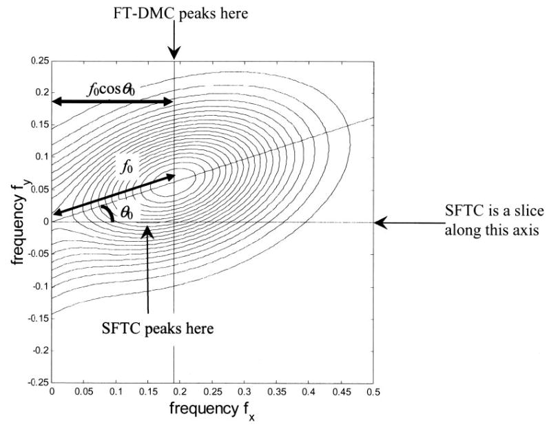
Contour plot of Fourier power spectrum for Gabor function oriented at 18° to vertical, tuned to frequency 0.2 cpd, spatial frequency bandwidth 1.5 octaves, and orientation bandwidth 30° (both full-width at half-maximum of power spectrum).

$$f_x=\frac{{\sigma }_{\perp }^2}{[{\sigma }_{\perp }^2{cos}^2{\theta }_0+{\sigma }_{\parallel }^2{sin}^2{\theta }_0]}{f}_{0}cos{\theta }_0$$ (F3)

where σ_|| and σ_⊥ describe the extent of the Gabor, respectively, parallel and orthogonal to its preferred orientation. It follows that, provided σ_||, σ_⊥, misaligning the stimuli will cause the measured monocular SFTCs to peak at a lower frequency than the power spectrum of the disparity-tuning curve. Thus, at least for the class of model considered here, such misalignment cannot be responsible for the observation that the disparity frequency is usually lower than the preferred monocular spatial frequency.

APPENDIX G: GLOSSARY OF SYMBOLS USED IN THE APPENDICES

C	firing rate of model cell (e.g., Eq. C1)
δ	disparity along an axis orthogonal to receptive field orientation
D(δ)	disparity-modulated component of response to binocular random-dot patterns (Eq. D1)
$\tilde{D}(f)$	Fourier amplitude spectrum of the disparity-modulated component of the disparity tuning curve (Eq. D4)
f	spatial frequency (cycles per degree)
fg	spatial frequency of grating stimulus (Eq. C3)
I(x , y)	image luminance, relative to mean, as a function of retinal position (e.g., Eq. C3)
IL(x, y), I R(x, y)	left and right retinal images
Ig, I RD	maximum luminance of grating/random-dot pattern relative to the mean screen luminance (cf. Eqs. C3 and D2)
j	index used to enumerate subunits feeding into a cell (Eq. D5)
L, R	mean response to monocular random-dot patterns in left, right eye (Eq. D7)
LSF(f ), R SF(f )	monocular spatial frequency tuning curve (i.e., response as a function of frequency to drifting gratings in left, right eyes; Eq. E1)
LASF , RASF	area under monocular SFTCs (Eq. E2)
Pos	half-wave rectification: Pos(x) ≡ x if x > 0, = 0 otherwise
ρ(x , y)	receptive field function
$\tilde{\rho }(\tilde{f},\tilde{\theta })$	Fourier transform of receptive field (polar coordinates; $\tilde{f},\tilde{\theta }$ are the spatial frequency and orientation of each Fourier component)
${\tilde{\rho }}^C({\tilde{f}}_x,{\tilde{f}}_y)$	Fourier transform of receptive field (Cartesian coordinates; ${\tilde{f}}_x,{\tilde{f}}_y$ are the components of spatial frequency orthogonal and parallel to the preferred orientation)
${\tilde{\rho }}^x({\tilde{f}}_x),{\tilde{\rho }}^y({\tilde{f}}_y)$	Fourier transform of one-dimensional receptive field profiles along axes orthogonal and parallel to the preferred orientation
θg	orientation of grating stimulus relative to the preferred orientation of the cell (Eq. C3 )
U	mean response to binocularly uncorrelated random-dot patterns (Eq. E8)
υL, υR	inner product (convolution) of retinal image with receptive field in left eye, right eye (Eq. C2)
x, y	retinal coordinates, in a frame where the y-axis is the preferred orientation of the cell

References

- Adelson EH, Bergen JR. Spatiotemporal energy models for the perception of motion. J Opt Soc Am A. 1985;2:284–299. doi: 10.1364/josaa.2.000284. [DOI] [PubMed] [Google Scholar]
- Anzai A, Ohzawa I, Freeman RD. Neural mechanisms for processing binocular information. II. Complex cells. J Neurophysiol. 1999a;82:909–924. doi: 10.1152/jn.1999.82.2.909. [DOI] [PubMed] [Google Scholar]
- Anzai A, Ohzawa I, Freeman RD. Neural mechanisms for processing binocular information. I. Simple cells. J Neurophysiol. 1999b;82:891–908. doi: 10.1152/jn.1999.82.2.891. [DOI] [PubMed] [Google Scholar]
- Barlow HB, Blakemore C, Pettigrew JD. The neural mechanisms of binocular depth discrimination. J Physiol. 1967;193:327–342. doi: 10.1113/jphysiol.1967.sp008360. [DOI] [PMC free article] [PubMed] [Google Scholar]
- Bridge H, Cumming BG. Responses of macaque V1 neurons to binocular orientation differences. J Neurosci. 2001;21:7293–7302. doi: 10.1523/JNEUROSCI.21-18-07293.2001. [DOI] [PMC free article] [PubMed] [Google Scholar]
- Cumming B, Parker A. Local disparity not perceived depth is signaled by binocular neurons in cortical area V1 of the macaque. J Neurosci. 2000;20:4758– 4767. doi: 10.1523/JNEUROSCI.20-12-04758.2000. [DOI] [PMC free article] [PubMed] [Google Scholar]
- Cumming BG. An unexpected specialization for horizontal disparity in primate primary visual cortex. Nature. 2002;418:633– 636. doi: 10.1038/nature00909. [DOI] [PubMed] [Google Scholar]
- Cumming BG, DeAngelis GC. The physiology of stereopsis. Annu Rev Neurosci. 2001;24:203–238. doi: 10.1146/annurev.neuro.24.1.203. [DOI] [PubMed] [Google Scholar]
- Cumming BG, Parker AJ. Responses of primary visual cortical neurons to binocular disparity without depth perception. Nature. 1997;389:280–283. doi: 10.1038/38487. [DOI] [PubMed] [Google Scholar]
- Cumming BG, Parker AJ. Binocular neurons in V1 of awake monkeys are selective for absolute, not relative, disparity. J Neurosci. 1999;19:5602–5618. doi: 10.1523/JNEUROSCI.19-13-05602.1999. [DOI] [PMC free article] [PubMed] [Google Scholar]
- Dean AF. The variability of discharge of simple cells in the cat striate cortex. Exp Brain Res. 1981;44:437– 440. doi: 10.1007/BF00238837. [DOI] [PubMed] [Google Scholar]
- DeAngelis GC, Ohzawa I, Freeman R. Depth is encoded in the visual cortex by a specialised receptive field structure. Nature. 1991;352:156–159. doi: 10.1038/352156a0. [DOI] [PubMed] [Google Scholar]
- de Valois RL, Albrecht DG, Thorell LG. Spatial frequency selectivity of cells in macaque visual cortex. Vision Res. 1982;22:545–559. doi: 10.1016/0042-6989(82)90113-4. [DOI] [PubMed] [Google Scholar]
- Efron B. Bootstrap methods: another look at the jackknife. Ann Stat. 1979;7:1–26. [Google Scholar]
- Fleet D, Wagner H, Heeger D. Neural encoding of binocular disparity: energy models, position shifts and phase shifts. Vision Res. 1996;36:1839–1857. doi: 10.1016/0042-6989(95)00313-4. [DOI] [PubMed] [Google Scholar]
- Foley JD, Dam Av, Feiner SK, and Hughes JF.Computer Graphics: Principles and Practice. Reading, MA: Addison–Wesley, 1990.
- Hammond P, Pomfrett CJ. Interocular mismatch in spatial frequency and directionality characteristics of striate cortical neurones. Exp Brain Res. 1991;85:631– 640. doi: 10.1007/BF00231749. [DOI] [PubMed] [Google Scholar]
- Lippert J, Wagner H. A threshold explains modulation of neural responses to opposite-contrast stereograms. Neuroreport. 2001;12:3205–3208. doi: 10.1097/00001756-200110290-00013. [DOI] [PubMed] [Google Scholar]
- Livingstone MS, Tsao DY. Receptive fields of disparity-selective neurons in macaque striate cortex. Nat Neurosci. 1999;2:825– 832. doi: 10.1038/12199. [DOI] [PubMed] [Google Scholar]
- Nikara T, Bishop PO, Pettigrew JD. Analysis of retinal correspondence by studying receptive fields of binocular single units in cat striate cortex. Exp Brain Res. 1968;6:353–372. doi: 10.1007/BF00233184. [DOI] [PubMed] [Google Scholar]
- Ohzawa I. Mechanisms of stereoscopic vision: the disparity energy model. Curr Opin Neurobiol. 1998;8:509–515. doi: 10.1016/s0959-4388(98)80039-1. [DOI] [PubMed] [Google Scholar]
- Ohzawa I, DeAngelis G, Freeman R. Stereoscopic depth discrimination in the visual cortex: neurons ideally suited as disparity detectors. Science. 1990;249:1037–1041. doi: 10.1126/science.2396096. [DOI] [PubMed] [Google Scholar]
- Ohzawa I, DeAngelis G, Freeman R. Encoding of binocular disparity by complex cells in the cat’s visual cortex. J Neurophysiol. 1997;77:2879–2909. doi: 10.1152/jn.1997.77.6.2879. [DOI] [PubMed] [Google Scholar]
- Ohzawa I, DeAngelis G, Freeman RD. Encoding the binocular disparity by simple cells in the cat’s visual cortex. J Neurophysiol. 1996;75:1779–1805. doi: 10.1152/jn.1996.75.5.1779. [DOI] [PubMed] [Google Scholar]
- Ohzawa I, Freeman RD. The binocular organization of complex cells in the cat’s visual cortex. J Neurophysiol. 1986a;56:243–259. doi: 10.1152/jn.1986.56.1.243. [DOI] [PubMed] [Google Scholar]
- Ohzawa I, Freeman RD. The binocular organization of simple cells in the cat’s visual cortex. J Neurophysiol. 1986b;56:221–242. doi: 10.1152/jn.1986.56.1.221. [DOI] [PubMed] [Google Scholar]
- Poggio GF, Fischer B. Binocular interaction and depth sensitivity of striate and prestriate cortex of behaving rhesus monkey. J Neurophysiol. 1977;40:1392–1405. doi: 10.1152/jn.1977.40.6.1392. [DOI] [PubMed] [Google Scholar]
- Prince SJ, Cumming BG, Parker AJ. Range and mechanism of encoding of horizontal disparity in macaque V1. J Neurophysiol. 2002a;87:209–221. doi: 10.1152/jn.00466.2000. [DOI] [PubMed] [Google Scholar]
- Prince SJ, Pointon AD, Cumming BG, Parker AJ. Quantitative analysis of the responses of V1 neurons to horizontal disparity in dynamic random-dot stereograms. J Neurophysiol. 2002b;87:191–208. doi: 10.1152/jn.00465.2000. [DOI] [PubMed] [Google Scholar]
- Qian N. Computing stereo disparity and motion with known binocular cell properties. Neural Comput. 1994;6:390– 404. [Google Scholar]
- Qian N, Zhu Y. Physiological computation of binocular disparity. Vision Res. 1997;37:1811–1827. doi: 10.1016/s0042-6989(96)00331-8. [DOI] [PubMed] [Google Scholar]
- Read JCA. A Bayesian model of stereopsis depth and motion direction discrimination. Biol Cybern. 2002;86:117–136. doi: 10.1007/s004220100280. [DOI] [PubMed] [Google Scholar]
- Read JCA, Parker AJ, Cumming BG. A simple model accounts for the reduced response of disparity-tuned V1 neurons to anti-correlated images. Vis Neurosci. 2002;19:735–753. doi: 10.1017/s0952523802196052. [DOI] [PubMed] [Google Scholar]
- Smith EL, 3rd, Chino YM, Ni J, Ridder WH, 3rd, Crawford ML. Binocular spatial phase tuning characteristics of neurons in the macaque striate cortex. J Neurophysiol. 1997;78:351–365. doi: 10.1152/jn.1997.78.1.351. [DOI] [PubMed] [Google Scholar]
- Tsai JJ, Victor JD. Reading a population code: a multi-scale neural model for representing binocular disparity. Vision Res. 2003;43:445– 466. doi: 10.1016/s0042-6989(02)00510-2. [DOI] [PubMed] [Google Scholar]