Assessing lung cancer risk in railroad workers using a first hitting time regression model

SUMMARY

This article examines the application of a first hitting time (FHT) model, using an operational time scale, to assess mortality risk differentials of the work environment. A major case application is presented that applies the model to three job categories of railroad workers. The data set involves a study of more than 50 000 workers with mortality assessed from 1959 to 1996. Lung cancer mortality was assessed because of a suspected link to diesel exhaust exposure. Based on a model that stipulates that death occurs when the disease state of a subject first hits a threshold value, the FHT model provides insights into factors influencing disease progression. In this application, in particular, the findings suggest that a job category in 1959 alters the risk of death from lung cancer.

1. INTRODUCTION

There is much scientific interest in knowing if the work environment elevates risk for certain diseases. This study was initiated by the concern that exposure to diesel exhaust may increase the risk of contracting lung cancer. Numerous studies have suggested that workers in occupations where diesel exhaust exposure occurred had an elevated risk of lung cancer (Health Effects Institute, 1995). Railroad engineers, conductors, and brakemen in the U.S. have had workplace exposure to diesel exhaust since diesel-powered locomotives replaced steam-powered locomotives after World War II. By 1959, U.S. railroads had almost completely converted to diesel power. Our research group has previously conducted a case-control study (Garshick et al., 1987) and a retrospective cohort study in U.S. railroad workers assessing mortality between 1959 and 1980 (Garshick et al., 1988; Larkin et al., 2000). These studies indicated that workers with jobs associated with operating trains have an elevated lung cancer risk. We have recently updated the mortality experience of the retrospective cohort through 1996, thereby providing 38 years of mortality follow-up of diesel-exposed workers. Details of the mortality update will be presented elsewhere (Garshick et al., in preparation).

The principal methods of analysis used in the earlier studies of this data set included Cox proportional hazards and Poisson regression. In this article, we employ a first hitting time regression model to analyze the relationship between work in diesel-exposed jobs and lung cancer mortality. These newer kinds of survival models and methods can provide additional insights into occupational mortality studies.

2. STUDY COHORT

The study cohort includes 54 973 white males who had worked in the railroad industry for 10 to 20 years prior to 1959, the baseline year. As already noted, 1959 roughly corresponds to the complete conversion to diesel-power in U.S. railroads. There is an interest in knowing the relationship between job category and years of work in a diesel-exposed job with lung cancer mortality. The U.S. Railroad Retirement Board (RRB) provided yearly railroad job codes between 1959 and retirement or death through 1996. Work environments in our data set are relatively distinct across three principal job categories: (i) train operations personnel, such as engineers, firemen, brakemen, conductors, and hostlers (called the engineer-brakeman group); (ii) railroad shop workers, such as machinists, electricians and shop supervisors; and (iii) other employees such as clerks, ticket agents, station agents and signal maintainers. In terms of work environments and exposure to diesel exhaust, the engineer-brakeman category would experience exposure while serving on operating trains. Although diesel repair shop workers experienced potentially higher exposures, the job codes selected for inclusion in this study included non-diesel repair shop workers. Therefore, it is not possible to define the diesel exposures of these workers. The other workers would have infrequent or no exposure. Mortality was assessed from 1959 through 1996 using information provided by the RRB, Healthcare Financing Administration, and Social Security System. Time until death or end of the study period was measured for each subject. Cause of death was based on diagnoses obtained by either death certificate review or National Death Index, allowing the identification of lung cancer and other causes. No individual level information was available on smoking or other covariates. We consider the following baseline covariates in this report: age in 1959 (variable age59) and job category in 1959 (engineer-brakeman, variable eb59; shop worker, variable shop59; other worker, variable other59) as risk factors for lung cancer mortality. We also consider the cumulative exposure covariates representing total time (in years) employed in each of the three job categories between 1959 and 1996 (engineer-brakeman, variable ebtot; shop worker, variable shoptot; other worker, variable othertot). An analysis of the data shows that almost all workers remained in the same job category from 1959 until the end of their working life.

The initial selection of models has been based on a subsample consisting of 20 per cent of subjects drawn randomly from the full data set by the project scientific team. Thus, a large hold-out sample (80 per cent) has been reserved for the confirmatory analysis presented in this report.

3. FIRST HITTING TIME MODEL

The first hitting time (FHT) model describes fluctuations in health status by a stochastic process and survival time by the first passage time of the process sample path to a threshold. Parameters of the process and threshold are related to study covariates by generalized regression link functions. Censored survival events are accommodated by the models. Whitmore (1983), Whitmore et al. 1998, and Lee and Whitmore (1993, 2000, 2003), and cited references therein provide technical background regarding the general application of the FHT model. These models have been used in medical research, including the assessment of risk factors for AIDS (Lee et al., 2000), of cognitive decline and Alzheimer’s disease (Hashemi et al., 2003), and of factors influencing hospital stays (Horrocks and Thompson, 2004), among others.

To our knowledge, the FHT model has not been applied previously to the study of mortality in relation to occupational exposures. The potential advantages of the FHT model in occupational mortality studies are provided by a modeling structure that is (i) flexible in accommodating a wide variety of random and systematic effects that characterize occupational influence on mortality and (ii) realistic in descibing the mechanism of disease progression and death. Both advantages arise from the fact that a first passage time for a health status process is a compelling conceptual framework for the dynamic process defining a medical end-point, such as death. An added useful feature, which is a research innovation in this application, is the use of cumulative exposure to convert the calendar time scale (i.e. the time between 1959 and 1996 in our study) to an operational time scale. The operational time feature of the model adds further realism and enrichment because occupational exposures and disease progression do not mark time as steadily as a clock or calendar but advance in a random and uneven manner. A further advantage of the proposed FHT model is that it does not require the proportional hazards assumption of conventional Cox regression models, the most widely used competing model. (See Bagdonavicc̆ius and Nikulin, 2000, for example, for a discussion of this model and others that have generalized the Cox model to accommodate cumulative damage or exposure measures.)

We choose a Wiener diffusion process to model the latent health status process. We choose a Wiener process because this kind of process has been found to be a suitable model for many physical processes that exhibit random variation over time. It is also realistic for describing health status because, although health will tend to deteriorate as people age, on a smaller time scale it is prone to fluctations that may well be described by the bidirectional movements of a Wiener process. Because of its wide applicability and tractability, we have the additional advantage of being able to use the technical developments for Wiener processes found in previous published work.

The essential structure of the FHT model for a Wiener process is illustrated in Figure 1. This model views health status as a latent (i.e. unobservable) stochastic process {X(r)}. The reason for our use of r to denote the time parameter will be explained further. At the outset of observation (time r = 0), the health status has an unknown initial level X(0) = x₀ > 0. Death occurs when the sample path first hits level zero, which we refer to as the absorbing threshold. We denote this first passage time by S. Thus, S = min{r : X(r) ≤ 0}. Such an occurrence is illustrated by path 1 in Figure 1. There is no assurance that the sample path will reach the absorbing threshold by the end of follow-up at time L (e.g. the end of the study period). In this case, the outcome is a censored survival time of L. This situation is illustrated by path 2 in Figure 1. Figure 2 shows four simulated sample paths of a Wiener process having parameter values of a typical subject in the case study described later. The baseline age is 40. Only one of the four sample paths reaches the absorbing threshold at zero before age 90. For this one path, death from lung cancer, for example, occurs at an age just above 63.

Figure 1.

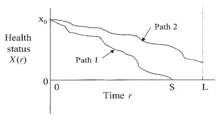
Two illustrative sample paths of health status starting from initial level x₀ until failure at time S (path 1) or end of follow-up at time L (path 2)

Figure 2.

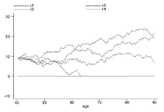
Four illustrative sample paths for a typical subject under the first hitting time model. The lower path crosses the zero-threshold just above 63 years of age, leading to the subject’s death from one specific cause

The stochastic process and threshold have three subject-level parameters, namely the initial level x₀ and the mean μ_x and variance σ_xx of the Wiener process. These parameters, taken together, define the trajectory of the health status sample path of a subject. The initial level x₀ sets the starting point for the trajectory. The farther it is from the threshold at zero the greater is the initial health of the subject with respect to the disease under study (lung cancer here). The mean parameter μ_x describes the rate per unit time at which the sample path approaches the threshold. Finally, σ_xx represents the inherent variability per unit time of the sample path and gives the model its random or stochastic behavior. The smaller σ_xx the more predictable the subject’s health outcome. The three parameters work in unison to determine if the sample path approaches the threshold and, if so, its rate of approach and, hence, the subject’s survival prospects.

There are several properties of this FHT model that will be relevant for understanding the analysis and interpreting the findings.

1. The first hitting time S for a Wiener process has an inverse Gaussian distribution. The inverse Gaussian probability density function is given by

   $$f(s|x_0,{\mu }_x,{\sigma }_{xx})\mathrm{\hspace{0.17em} }=\mathrm{\hspace{0.17em} }\frac{x_0}{{(2\pi {\sigma }_{xx}{s}^3)}^{1/2}}\text{exp}\left[–\frac{{(x_0+{\mu }_{x}s)}^2}{2{\sigma }_{xx}s}\right]$$ (1)

   The survival function of S, representing the complementary cumulative distribution function P(S > s), has the form

   $$\overline{F}(s|x_0,{\mu }_x,{\sigma }_{xx})\mathrm{\hspace{0.17em} }=\mathrm{\hspace{0.17em} }\Phi \left[({\mu }_{x}s+x_0){({\sigma }_{xx}s)}^{–1/2}\right]\mathrm{\hspace{0.17em} }–\mathrm{\hspace{0.17em} }\text{exp\hspace{0.17em}}(–\text{2}{x}_0{\mu }_x / {\sigma }_{xx})\Phi \left[({\mu }_{x}s–x_0){({\sigma }_{xx}s)}^{–1/2}\right]$$ (2)

   where Φ(·) denotes the cumulative distribution function of the standard normal distribution. These functions are set out in standard references such as Chhikara and Folks (1989). Both of these functions are needed to estimate the model parameters.

2. For a Wiener process, it can be shown that the threshold will eventually be reached with probability 1 (i.e. death from the specific cause will occur eventually) if μ_x is negative, so the process tends to drift toward the threshold at zero. The same is true if μ_x = 0. If μ_x is positive, so the process tends to drift away from the threshold at zero, then reaching the threshold is not certain. The possibility of no absorption might appear paradoxical at first because it seems to offer a positive probability of avoiding death if μ_x > 0. The apparent paradox is explained, however, by noting that we are considering only one specific cause of death (e.g. lung cancer) and there is no certainty of dying from that specific cause even when other causes are ignored or suspended. The model considers the competing risks of different causes of death by allowing survival time for one cause to be censored by other causes of death. If we let D_L denote the event of eventual death from lung cancer when competing causes of death are ignored, then the probability of absorption is given by the following formula, which may be obtained from (2) by letting s increase without limit:

   $$P(D_L)\mathrm{\hspace{0.17em} }=\mathrm{\hspace{0.17em} }\{\begin{array}{lll}1\hfill & \text{for}\hfill & {\mu }_x\hspace{0.17em}\le \hspace{0.17em}0\hfill \\ \text{exp}(–\text{2}{x}_0{\mu }_x/{\sigma }_{xx})\hfill & \text{for}\hfill & {\mu }_x\hspace{0.17em}>\hspace{0.17em}0\hfill \end{array}$$ (3)

   The event D_L is a potentially latent or unobservable death as described in the conventional competing risks literature (see, for example, Kalbfleisch and Prentice, 1980, Chapter 7).

3. The mean survival time, conditional on event D_L, is given by

   $$\text{E}(S|D_L)\mathrm{\hspace{0.17em} }=\mathrm{\hspace{0.17em} }\frac{x_0}{\left|{\mu }_x\right|}\mathrm{\hspace{0.17em} }\mathrm{\hspace{0.17em} }\mathrm{\hspace{0.17em} }\text{for\hspace{0.28em}}\mathrm{\hspace{0.17em} }\mathrm{\hspace{0.17em} }{\mu }_x\hspace{0.17em}\ne \hspace{0.17em}0$$ (4)

   Thus, E(S | D_L) is the expected time to absorption for subjects whose sample path reaches the threshold for this cause of death.

4. The health status process has a scale with an origin at zero (where death occurs) but an arbitrary unit interval. We fix the unit interval of the health status scale by setting the variance parameter to unity, i.e. σ_xx = 1. As we have set σ_xx = 1, we note that probability P(D_L) in (3) depends only on the product x₀μ_x when μ_x > 0. The larger this product (when it is positive), the lower the risk of death from the specific cause.

5. The parameters x₀ and μ_x can be linked to relevant baseline covariates, including baseline age and job category, using appropriate link functions. We let z denote the vector of baseline covariates for a subject and β and γ be vectors of regression parameters. We adopt the following identity and logarithmic link functions for μ_x and x₀, respectively:

$${\mu }_x\mathrm{\hspace{0.17em} }=\mathrm{\hspace{0.17em} }z\beta$$ (5)

$$\text{ln\hspace{0.17em}}(x_0)\mathrm{\hspace{0.17em} }=\mathrm{\hspace{0.17em} }z\gamma$$ (6)

4. THE OPERATIONAL TIME SCALE

We now introduce the concept of operational time to the preceding model. Operational time is to be distinguished from calendar time. The calendar marks off time in months and years. In contrast, operational time measures the cumulative exposure of a system to aggregate physical effects that cause its deterioration. In our application, we are concerned with the aggregate effects of living on the health status of a subject. The aggregate effects may relate to a single cause of death, such as lung cancer, or multiple competing causes of death, depending on the context. Thus, operational time is not measured in terms of months or years but in units of accruing risk for disease and death. The more slowly operational time accrues, the longer the subject postpones potential death from the disease. Different time intervals during life will increase or decrease the accrual rate depending on the disease risk and health stress to which the subject is exposed during the interval. A useful analogy can be drawn with operating an automobile. The calendar age of an automobile is measured in years. Its operational age would be measured by its cumulative use or distance driven (i.e. accumulated mileage). The assumption is that physical wearout is related more to usage than the simple passage of time.

Returning to our model, if calendar time is represented by t, then operational time is a monotonic stochastic process {R(t)}, where R(t) = r states that the cumulative exposure to disease equals r by calendar time t. We take the health status process {X(r)} as a Wiener process defined on the operational time scale (as described above). The combined stochastic process {X[R(t)]} is called a subordinated process, with {X(r)} being the parent process and {R(t)} being the directing process.

In our case application, operational time is defined by the cumulative exposure to different work environments in job categories that a subject holds during his life span. For completeness, we treat retirement as one of these categories. To be precise, let {I_j(t)} be an indicator process for a subject defined as follows:

$$I_j(t)\mathrm{\hspace{0.17em} }=\mathrm{\hspace{0.17em} }\{\begin{array}{cc}1& \text{if\hspace{0.17em}the\hspace{0.17em}subject}\text{'}\text{s\hspace{0.17em}job\hspace{0.17em}category\hspace{0.17em}is\hspace{0.17em}}j\hspace{0.17em}\text{at\hspace{0.17em}time\hspace{0.17em}}t\\ 0& \text{otherwise}\end{array}.$$ (7)

The directing process {R(t)}, representing the operational time of a subject, is related to these indicator processes as follows:

$$R(t)\mathrm{\hspace{0.17em} }=\mathrm{\hspace{0.17em} }\sum _{j=1}^J{\int }_0^t{\alpha }_j{I}_j\left(u\right)\text{d}u\mathrm{\hspace{0.17em} }=\mathrm{\hspace{0.17em} }\sum _{j=1}^J{\alpha }_j{A}_j(t)$$ (8)

where A_j(t) denotes the total time employed in job category j by time t. The interval A_j(t) will be observable for each subject. The α_j, j = 1, . . . , J, are positive parameters that are to be estimated. These parameters are assumed to be the same for all subjects. In advance of observation, the A_j(t) are random variables. Denoting their realizations in the study by A_j(t) = a_j(t), the function defining realized operational time, i.e. R(t) = r(t), is given by

$$r(t)\mathrm{\hspace{0.17em} }=\mathrm{\hspace{0.17em} }\sum _{j=1}^J{\alpha }_j{a}_j(t)$$ (9)

Each time interval a_j(t), j = 1, . . . , J, contributes to cumulative exposure at a rate α_j > 0. As the operational time scale is arbitrary up to a constant, we set the rate for the Jth job category to unity (i.e. α_J = 1). Hence, job category J represents the numeraire or reference time unit for the operational scale. The selection of the numeraire is largely arbitrary. In our case application, category J will represent retirement. In our application of (9), we take the intervals a_j(t) as known intervals of employment in different job categories, including retirement as a final category. If a subject dies while employed or is employed at the end of the study period then, of course, a_J(t) = 0. Observe from (9) that r(0) = 0 and that r(t) is a monotonic sample path.

Figure 3 illustrates the relationship between operational time and calendar time for a simple setting. In this illustration, the subject works three consecutive intervals in three different jobs during the total interval [t₀, t], where t₀ = 0. The intervals are denoted by a₁(t) = [t₀, t₁), a₂(t) = [t₁, t₂) and a₃(t) = [t₂, t] in the figure. Equation (9) has the following form in this illustration:

Figure 3.

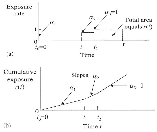
Relation of operational time r(t) (cumulative exposure) to calendar time t: (a) exposure occurs at different rates in consecutive intervals; (b) comparative time scales: exposure occurs at different rates in consecutive intervals

$$r(t)\mathrm{\hspace{0.17em} }=\mathrm{\hspace{0.17em} }\sum _{j=1}^2{\alpha }_j(t_j–t_{j–1})\hspace{0.17em}+\hspace{0.17em}(t–t_2)$$ (10)

Figure 3(a) shows the rate function as a series of blocks having different elevations, defining the α_j parameters. Figure 3(b) shows the integrated rates giving the comparative time scales r versus t. In this illustration the cumulative exposure rate is lower in earlier years while the subject is still actively employed (intervals [t₀, t₁) and [t₁, t₂) in the figure), whereas the exposure rate rises to 1 during retirement (interval [t₂, t] in the figure). This setup is consistent with the healthy-worker survivor effect that will be encountered in the case study taken up shortly.

5. MODEL ESTIMATION

Our analysis here corresponds to inverse Gaussian regression for censored survival data with an operational time feature. The methodology extends that described in Whitmore (1983). We use maximum likelihood methods for estimating the model parameters. We have an observation triplet (t_i, d_i, z_i) for each subject i, i = 1, . . . , n. Here t_i denotes the time to death from lung cancer, time to death from another cause or end of the study period (measured in calendar time); d_i is an indicator for lung cancer death (d_i = 1) or a censored observation (d_i = 0); and z_i is the subject’s covariate vector. We treat death from other causes as a right-censoring event that occurs completely at random.

The link between calendar time t_i and operational time r_i for each subject i is made as follows, using the relationship in (9):

$$r_i\mathrm{\hspace{0.17em} }=\mathrm{\hspace{0.17em} }\sum _{j=1}^J{\alpha }_j{a}_j^{\left(i\right)}(t_i)$$ (11)

Here a⁽ⁱ⁾_j(t_i) is the time spent by subject i in job category j in interval [0, t_i]. We represent the vector of parameters α_j, j = 1,. . . , J, in (11) by α. The α parameters will enter the sample likelihood function in the logarithmic form ln(α_j) to ensure positive parameter estimates.

As z_i denotes the vector of baseline covariates for subject i, the subject has unique parameter values μ⁽ⁱ⁾_x and x⁽ⁱ⁾₀ defined by the link functions given earlier, namely, μ⁽ⁱ⁾_x = z_iβ and ln(x⁽ⁱ⁾₀) = z_iγ.

A subject i who dies from lung cancer during the study period contributes survival probability density f(r_i | μ⁽ⁱ⁾_x, x⁽ⁱ⁾₀) to the sample likelihood function. A subject i who dies from another cause or survives to the end of the study period contributes probability $\overline{F}(r_i|{\mu }_x^{(i)},x_0^{(i)})$ to the sample likelihood function. These functions were defined earlier in (1) and (2). Observe that the functions are now defined in terms of operational time r. The sample log-likelihood function to be maximized has the form:

$$\text{ln\hspace{0.17em}}L(\alpha ,\beta ,\gamma )\mathrm{\hspace{0.17em} }=\mathrm{\hspace{0.17em} }\sum _{i=1}^n\left\{d_{i}lnf(r_i|{\mu }_x^{\left(i\right)},x_0^{\left(i\right)})\hspace{0.17em}+\hspace{0.17em}\left(1–d_i\right)\hspace{0.17em}ln\hspace{0.17em}\overline{F}(r_i|{\mu }_x^{\left(i\right)},x_0^{\left(i\right)})\right\}$$ (12)

We use a built-in numerical optimization routine in the STATA software system to obtain the maximum likelihood estimates. The negative of the inverse Hessian matrix for the log-likelihood function, evaluated at its maximum, provides an estimate of the asymptotic covariance matrix of the parameter estimates. The optimization gives estimates of the mean parameter μ⁽ⁱ⁾_x and the initial health level x⁽ⁱ⁾₀ for each subject i.

Because the Wiener process involves parametric assumptions (e.g. normality, independent increments) that may not be met fully, we complement the asymptotic inferences provided by a standard log-likelihood analysis with inferences drawn from a random partition of subsets of the data set. Specifically, we partition the full data set into m subsets of equal size. The model parameter estimates are then computed for each subset using (12). The resulting parameter estimates constitute a simple random sample from a common sampling distribution (of unspecified form). If m is sufficiently large (we use m = 25), the central limit theorem ensures that the means of the m estimates will be approximately normally distributed (more precisely, jointly multivariate normal). Normal theory may therefore be used confidently to make inferences.

The preceding model assumes that the survival distribution will be the same for all subjects who share the same covariate vectors. Thus, the model does not accommodate potential heterogeneity among subjects having the same baseline characteristics and job exposures. A potential extension of the model is one where the regression function for each parameter has a random intercept. The extension is left for future development.

6. LUNG CANCER MORTALITY—ANALYSIS AND FINDINGS

A censored survival data analysis was carried out using the likelihood function in (12). Our analysis employed covariates for age in 1959 (variable age59) and job category in 1959 (engineer-brakeman, variable eb59; shop worker, variable shop59; and other worker, variable other59) in link functions (5) and (6). Operational time in (9) considered intervals of employment as an engineer-brakeman (variable ebtot), shop worker (variable shoptot) and other worker (variable othertot). Job intervals are measured in years. As age in 1959 is incorporated as a covariate, the calendar time scale represents the subject’s age in years, measured from 1959.

Maximum likelihood estimates of the regression coefficients were obtained for the full sample. The estimates and their asymptotic P-values are reported in the first two number columns in Table 1. Table 1 also shows, in the last two columns, mean point estimates and P-values for the parameter estimates calculated from the m = 25 random subsets. The P-values are computed using a t distribution with m − 1 = 24 degrees of freedom. It can be seen that these non-parametric subsample mean estimates are generally similar to those provided by the maximum likelihood method when the full data set is analyzed. The asymptotic P-values from the full likelihood analysis are generally smaller than their non-parametric subsample counterparts, lending support to our caution to validate our inferences using a non-parametric approach. We will use the full-sample parameter estimates in the following discussion of the findings, giving additional attention to the non-parametric results where there is a material difference.

Table 1.

Regression output for the FHT model for lung cancer death, using both the full data set and distribution-free inferences from a random partition of m = 25 subsets

		Results based on full data set		Results based on data subsets
Estimated model parameters		Estimate	P-value	Estimate	P-value
ln(x0): Logarithm of initial health status
Regression covariates	age59	−0.01916	0.000	−0.01907	0.000
	eb59	−0.10569	0.000	−0.10618	0.022
	shop59	0.05757	0.088	0.07971	0.156
	constant	2.53885	0.000	2.56046	0.000
μx: Mean health status
Regression covariates	age59	0.00375	0.000	0.00372	0.000
	eb59	−0.00578	0.566	−0.00671	0.669
	shop59	−0.02424	0.043	−0.03247	0.121
	constant	−0.00487	0.853	−0.00926	0.813
ln(α): Log-exposure rate
Regression covariates	ebtot	−1.5528	0.000	−1.5399	0.000
	shoptot	−1.0909	0.000	−1.1116	0.000
	othertot	−1.3264	0.000	−1.3491	0.000

In interpreting the findings in Table 1, it is important to bear in mind that the health status being considered in this analysis is in relation to lung cancer. It is also important to remember that time is being measured on an operational time scale. Conversion to calendar time may be done by finding that t for which r(t) = r using (9). As variables eb59, shop59 and other59 form a system of indicator variables, we have chosen the last as the reference job category. Thus, the effects of eb59 and shop59 shown in the table represent differential effects relative to the other59 job category. Table 1 provides the following findings:

1. The log-initial health status ln(x₀) is significantly affected by age59 and eb59, while parameter μ_x only has age59 as a significant covariate(shop59 is marginally significant). This finding implies that being in the engineer-brakeman job category in 1959 yields a significantly different health status trajectory than other job categories for a subject of any fixed age. As the indicator variable eb59 appears to affect x₀ but not μ_x, the difference is in the level of the sample path (as set by its initial starting point) and not its rate of change over time.

2. As age59 exceeds 40 for all subjects, the estimate of parameter μ_x is positive for all subjects. Remember that parameter μ_x represents change in health status with each unit increase in operational time. The positive value indicates that the probability of eventual death from lung cancer ignoring competing causes of death (i.e. event D_L) is less than one for all subjects.

3. Initial health status x₀ is estimated to decline with age59 at about 1.9 per cent per year of age. This effect is anticipated as older subjects should, on average, have a lower health status.

4. The estimates of initial health status x₀ and, hence, the conditional mean survival time E(S | D_L) are about 10.0 per cent lower when the subject was an engineer-brakeman in 1959 (eb59 = 1) rather than in the other-worker category (the reference category). Again, we remind the reader that E(S | D_L) is a point on the operational time scale. The eb59 effect is of the same magnitude based on the subsamples mean but the P-value is not as small, although it remains below the standard 0.05 level.

5. As for the exposure rates α, the regression output shows estimates of their natural logarithms (with P-values). Recall that the retirement category defines the numeraire or reference value here with parameter α_J = 1. We have reproduced the α_j estimates in Table 2 in their exponentiated form. The fractional value of the estimate ${\widehat{\alpha }}_j$ for each job category is indicative of a healthy-worker survivor effect, i.e. the effect whereby good health allows a person to continue in employment. For the engineer-brakeman category, for example, ln( ${\widehat{\alpha }}_1$) = −1.5528, which gives ${\widehat{\alpha }}_1$ = 0.212. This value implies that, for a subject employed as an engineer-brakeman, operational time progresses at about 21 per cent of the rate of a retired subject (the reference category). The values of ${\widehat{\alpha }}_j$ for the three job categories range from 0.212 to 0.336. Their small values show the slow progression of operational time for a subject who is employed relative to one who is retired. For a general reference on the topic of healthy worker survivor effect, see Arrighi and Hertz-Picciotto (1994).

Table 2.

Exposure rates (operational time parameters) for different job categories. The retirement interval is the numeraire with α_J = 1

Job category		Parameter estimates
j	Time aj(t)	${\widehat{\alpha }}_j$	ln( ${\widehat{\alpha }}_j$)
1	ebtot	0.212	−1.5528
2	shoptot	0.336	−1.0909
3	othertot	0.265	−1.3264

7. DISCUSSION

The FHT model is based on the concept that a lung cancer mortality event occurs when the disease state of a subject first hits a threshold value. The FHT model, defined for operational time, has been computationally easy to implement in this study and provides a rich, plausible and flexible modeling structure for the data. It may be considered as an alternative to the more traditional approaches of logistic and Cox proportional hazards regression modeling for occupational cohort mortality studies. We have initially used a standard parametric likelihood approach to estimate parameters from the full data set. This procedure was followed by a complementary procedure whereby the parametric model was used to generate parameter estimates for subsamples and then non-parametric inferences were drawn from the subsample estimates. The complementary approach has been shown to offer greater confidence in the study findings. The use of a large hold-out sample has also done its part to boost confidence that over-fitting was not a problem.

The data analysis conducted here is the first stage of a longer program of investigation of this data set. Our continuing research is delving into achieving a better understanding of the relationship between cumulative exposure, based on years of work in a job category, and lung cancer mortality. We are also investigating methods that adjust for the healthy-worker survivor effects that have been uncovered by the FHT model. The following list elaborates on a few points of interest that are receiving further attention.

1. The significant differential in initial health status between workers employed as engineer-brakemen and those employed in the other two job categories (see the coefficients for ln(x₀) and their P-values in Table 1) is receiving additional study. A simple interpretation of the findings would suggest that the mere fact that a subject is in the eb59 job category in 1959 could be enough to create the risk differential. However, the cause of this effect is not clear from these data. Possible explanations include: (i) pre-1959 employment exposures to particulate matter, carcinogens or toxins were sufficient to trigger or initiate lung disease; (ii) individuals with latent disease potential or unhealthy lifestyles are self-selected into the higher risk job category; or (iii) other job environment features contribute to mortality risk. With respect to pre-1959 exposures, all subjects had worked in the railroad industry for 10 to 20 years prior to 1959 and, therefore, engineer-brakemen may have had work-related exposures for a decade or more before that date. The present analysis has not considered the effect of working prior to 1959 or in specific operational time periods after 1959. Particulate exposures to combustion products from steam locomotives occurred, together with diesel exposure, during the transition period prior to 1959. The earlier diesel engines are likely to have had greater particulate emissions than later engines, and it is possible that early exposures were greater. Further analyses and research are needed to assess the role of work in diesel-exposed jobs in the years preceding death, compared to more distant exposures. It is possible that lung disease is initiated by early exposure, with later exposure perhaps being less influential once the disease process is set in motion.

2. An extended analysis of the data set suggests that the operational time coefficients for exposure in the three job classes (see Table 2) differ from each other significantly and, therefore, that type of job and the healthy-worker survivor effect may be intertwined. It would be premature, however, to draw this inference in this report because the precise implications and nuances need further investigation. For example, the potential for differences between early and late exposure need to be evaluated. Preliminary analysis also seems to show that whether or not a worker takes early retirement (before 65) seems to be a relevant consideration in refining the healthy-worker survivor effect. The FHT model, with operational time, allows us to separate the effects of baseline variables and exposure influences that operate over time. For example, the model can pull apart the different rates for operational time arising from different job categories (e.g. engineer-brakeman, shop worker, other worker) or different time segments (e.g. before or after age 65). A final complication that needs to be considered is that of a possible lag between exposure and onset of disease. As these remarks show, much further work is needed to draw out the subtleties of pre- and post-1959 job exposure.

3. Younger subjects in 1959 have a higher probability of surviving to the end of the study period in 1996. For example, 37 per cent of subjects aged 40–44 in 1959 are still living in 1996. In contrast, only 1 per cent of those aged 60–64 in 1959 are living. The influence of late onset diseases and illnesses in younger subjects is therefore not much at play in this analysis. Survival prospects for younger subjects may therefore be somewhat overstated. This observation has some implications for the reasonableness of the early exposure mechanism in explaining the triggering of the disease.

References

- Arrighi HM, Hertz-Picciotto I. The evolving concept of the healthy worker survivor effect. Epidemiology. 1994;5:189–196. doi: 10.1097/00001648-199403000-00009. [DOI] [PubMed] [Google Scholar]
- Bagdonavicc̆ius V, Nikulin M. On goodness-of-fit for the linear transformation and frailty models. Statistics and Probability Letters. 2000;47:177–188. [Google Scholar]
- Chhikara RS, Folks JL. 1989. The Inverse Gaussian Distribution: Theory, Methods, and Applications Marcel Dekker: New York.
- Garshick E, Schenker MB, Munoz A, Segal M, Smith TJ, Woskie SR, Hammond SK, Speizer FE. A case-control study of lung cancer and diesel exhaust exposure in railroad workers. Am Rev Respir Dis. 1987;135:1242–1248. doi: 10.1164/arrd.1987.135.6.1242. [DOI] [PubMed] [Google Scholar]
- Garshick E, Schenker MB, Munoz A, Segal M, Smith TJ, Woskie SR, Hammond SK, Speizer FE. A retrospective cohort study of lung cancer and diesel exhaust exposure in railroad workers. Am Rev Respir Dis. 1988;137(4):820–825. doi: 10.1164/ajrccm/137.4.820. [DOI] [PubMed] [Google Scholar]
- Hashemi R, Jacqmin-Gadda H, Commenges D. A latent process model for joint modeling of events and marker. Lifetime Data Analysis. 2003;9:331–343. doi: 10.1023/b:lida.0000012420.36627.a6. [DOI] [PubMed] [Google Scholar]
- Health Effects Institute. 1995. Diesel exhaust. A critical analysis of emissions, exposure, and health effects. Report, Diesel Working Group, Health Effects Institute.
- Horrocks J, Thompson ME. Modelling event times with multiple outcomes using the Wiener process with drift. Lifetime Data Analysis. 2004;10:29–49. doi: 10.1023/b:lida.0000019254.29153.1a. [DOI] [PubMed] [Google Scholar]
- Kalbfleisch JD, Prentice RL. 1980. The Statistical Analysis of Failure Time Data Wiley.
- Larkin EK, Smith TJ, Stayner L, Rosner B, Speizer FE, Garshick E. Diesel exhaust and lung cancer: adjustment for the effect of smoking in a retrospective cohort study. Am J Ind Med. 2000;38:399–409. doi: 10.1002/1097-0274(200010)38:4<399::aid-ajim5>3.0.co;2-d. [DOI] [PubMed] [Google Scholar]
- Lee MLT, Whitmore GA. Stochastic processes directed by randomized time. Journal of Applied Probability. 1993;30:302–314. [Google Scholar]
- Lee MLT, Whitmore GA. 2000. Assumptions of a latent survival model. In Goodness-of-Fit Tests and Model Validity Birkhauser: Boston; 227–236.
- Lee MLT, Whitmore GA. 2003. First hitting time models for lifetime data. In Handbook of Statistics, Vol. 23, Survival Analysis, Rao CR, Balakrishnan N (eds). Elsevier (to appear).
- Lee MLT, DeGruttola V, Schoenfeld D. A model for markers and latent health status. J Royal Statistical Society. 2000;62:747–762. [Google Scholar]
- Whitmore GA. A regression method for censored inverse-Gaussian data. Canadian Journal of Statistics. 1983;11:305–315. [Google Scholar]
- Whitmore GA, Crowder MJ, Lawless JF. Failure inference from a marker process based on a bivariate Wiener model. Lifetime Data Analysis. 1998;4:229–251. doi: 10.1023/a:1009617814586. [DOI] [PubMed] [Google Scholar]