Reconstruction of Cardiac Ventricular Geometry and Fiber Orientation Using Magnetic Resonance Imaging

Abstract

An imaging method for the rapid reconstruction of fiber orientation throughout the cardiac ventricles is described. In this method, gradient-recalled acquisition in the steady-state (GRASS) imaging is used to measure ventricular geometry in formaldehyde-fixed hearts at high spatial resolution. Diffusion-tensor magnetic resonance imaging (DTMRI) is then used to estimate fiber orientation as the principle eigenvector of the diffusion tensor measured at each image voxel in these same hearts. DTMRI-based estimates of fiber orientation in formaldehyde-fixed tissue are shown to agree closely with those measured using histological techniques, and evidence is presented suggesting that diffusion tensor tertiary eigenvectors may specify the orientation of ventricular laminar sheets. Using a semiautomated software tool called heartworks, a set of smooth contours approximating the epicardial and endocardial boundaries in each GRASS short-axis section are estimated. These contours are then interconnected to form a volumetric model of the cardiac ventricles. DTMRI-based estimates of fiber orientation are interpolated into these volumetric models, yielding reconstructions of cardiac ventricular fiber orientation based on at least an order of magnitude more sampling points than can be obtained using manual reconstruction methods.

INTRODUCTION

The three-dimensional spatial organization of the myofibers dictates many of the heart’s electrical and mechanical properties, influencing electrical propagation¹¹ and mechanical contraction.²⁵ Alterations in the normal myofiber architecture occur in diseases such as ischemic heart disease²⁶ and ventricular hypertrophy.¹² These alterations may predispose the myocardium to abnormal electrical propagation and arrhythmia.⁴ Therefore, a detailed quantification of the myofiber architecture of normal and diseased hearts would increase understanding of normal and abnormal cardiac electrical propagation and mechanical contraction.

There is now direct evidence that fiber inclination angles estimated using diffusion tensor magnetic resonance imaging (DTMRI) of short-axis sections of myocardium bathed⁷ or perfused¹⁸ in cardioplegic solution agree with those measured histologically. This finding suggests that DTMRI may provide a means for reconstructing fiber orientation throughout the ventricles, thereby avoiding time-consuming histological approaches.^15,22,24 However, application of this method to the three-dimensional reconstruction of cardiac fiber structure requires extended imaging times. Over such long time periods, we have observed that changes of ventricular geometry may occur using both the above preparations, especially during the first 12 h postexcision. The occurrence of this motion limits the amount of time available for DTMRI, and therefore the spatial resolution that may be achieved. Fixation of tissue would eliminate such motion, thereby providing longer imaging times and higher spatial resolution. We have demonstrated recently that estimates of cardiac fiber orientation obtained by computing the principle eigenvector of the diffusion tensor obtained by means of DTMRI in formaldehyde-fixed tissue agree with histological estimates obtained from the same tissue.⁵ Here, we apply this imaging method to the three-dimensional reconstruction of ventricular fiber orientation in the rabbit heart at high spatial resolution.

METHODS

Magnetic Resonance Imaging

Heart Extraction and Perfusion

New Zealand white male rabbits (2–4 kg) were anesthetized using ketamine (2 mg/kg iv), followed by heparin (1,000 U/kg iv) and were then exsanguinated. The thoracic cavity was opened, and the heart and lungs were rapidly excised and placed in a bath of cold (4 °C) cardioplegic solution. The aorta was cannulated, the lungs were ligated and removed, and the hearts were perfused retrogradely using a magnetic resonance (MR)-compatible Langendorff apparatus. The initial perfusate was a modified Krebs–Henseleit buffer containing (in mM) 118.0 NaCl, 25.0 NaHCO₃ , 5.0 dextrose, 4.6 KCl, 2.5 CaCl₂ , 1.2 KH₂PO₄ , and 1.0 MgSO₄ . Excess hydrostatic pressure accumulation resulting from thebesian drainage or aortic valvular insufficiency was relieved by a thin (1 mm o.d.) polyethylene tube inserted into the left ventricle (LV) through the mitral valve. Proper valve function was obtained by allowing the heart to beat several times. The heart was arrested by perfusing a modified St. Thomas’ Hospital solution that consisted (in mM) 110.0 NaCl, 10.0 NaHCO3, 5.0 dextrose, 16.0 KCl, 1.2 CaCl2, and 16.0 MgCl2 at room temperature (18 °C). Bovine serum albumin (3% wt./vol) was added to both perfusates to minimize formation of interstitial edema. A 95% O₂ –5% CO₂ gas mixture was allowed to continually equilibrate with both perfusates resulting in partial pressures of O₂ in excess of 600 mm Hg and a pH of 7.4. Following perfusion, 1/2 l of isotonic (3%) phosphate buffered formaldehyde was gravity fed through the aortic cannula to perfuse the coronary circulation over a period of ~30 min. The heart was then submerged in a container of the fixative, sealed, and stored for approximately 4 weeks.

GRASS and DTMR Imaging

Prior to imaging, hearts were suspended by the aortic cannula in a closed-end acrylic cylinder (31 mm o.d.) which was filled with the fixative solution. The cylinder also served as the housing for a loop-gap radio frequency (rf) coil. All imaging was performed on a 4.7 T MR scanner (GE Omega CSI, Fremont, CA). The loop-gap coil was tuned to proton resonance inside the scanner and B₀ homogeneity was optimized over the entire volume.

The following protocol was used to reconstruct ventricular geometry and fiber orientation. First, three-dimensional gradient recalled acquisition in the steady-state (GRASS) intensity images were collected for subsequent use in defining the epicardial and endocardial surfaces. Image size was 256×128×128 pixels. Given the field of view, this yielded a set of 128 short-axis slices with in-slice spatial resolution of 156×312 μm, and a slice separation of 469 μm.

Following acquisition of the GRASS intensity data set, DTMRI was used to estimate myocardial fiber orientation. These images were obtained using a slice-selective fast spin-echo diffusion-weighted technique followed by two-dimensional (2D) discrete Fourier transform. Figure 1 provides a schematic illustration of the pulse sequence. Diffusion weighting was provided by unipolar sinusoidal gradient pulses with 10 ms duration. The gradients were applied sequentially in six noncollinear directions with magnitudes of 6, 10, and 14 G/cm, and again with the same magnitudes but reversed polarity. A total of 36 images were obtained per slice, each with 256 readout steps (6.4 μs dwell time) and 128 phase-encoding steps, yielding in-plane resolution identical to that of the GRASS image data (156×312 μm). Image acquisition time was 96 s using a recycle time (TR) of 3 s, an echo train length of 8, and two signal averages per readout. This yielded a slice acquisition time of 1 h. Crusher gradients were not used on the initial 180° rf pulse, as the unipolar diffusion gradients served to spoil any transverse magnetization resulting from the free induction decay. Crusher gradients of 2 ms duration and varying magnitude (2–6 G/cm) were applied on either side of all subsequent 180° rf pulses. The variance in magnitude of the crushers served to spoil stimulated echo components of the signal.

FIGURE 1.

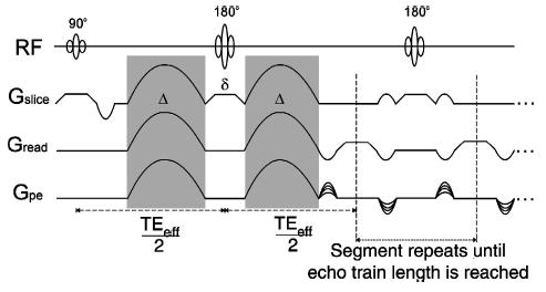
Diffusion-weighted fast spin-echo pulse sequence. The shaded regions denote the diffusion encoding gradients, which are of duration Δ and separated by time δ. The first diffusion-encoded echo is formed after slice selective 90° and 180° rf pulses at time TE_eff . Phase encoding is applied to subsequent echoes in the train, which are obtained by repeated refocusing with slice-selective 180° rf pulses, flanked by variable-amplitude crushers to minimize stimulated echo contributions. The first echoes of each train are used to fill the center of k space.

Slice thickness was varied depending on longitudinal position. In regions at and near the base of the heart where surface curvature is smallest, slice thickness was set to 2 mm. At more apical regions where curvature is larger, slice thickness was set to 1 mm. For the studies reported here, eight basal short-axis sections were obtained with a slice thickness of 2 mm, followed by 12 apical short-axis sections at a slice thickness of 1 mm. This protocol was selected as a tradeoff between total imaging time (~20 h) and spatial resolution, and yields one 256×128×128 matrix of intensity data which is used to estimate ventricular geometry, and a coincident 256×128×20 matrix of points at which estimates of the 3×3 diffusion tensor are available.

The relaxation times of fixed myocardium is dramatically shorter than that of perfused myocardium. This effect has been noted in other tissues as well, specifically the liver and spleen.²³ To determine appropriate values for TR and the effective echo time (TE_eff-time to the first echo) in fixed myocardium, we estimated T₁ and T₂ using a linescan technique.¹ Nonlinear least-squares regression was performed on sets of measurements, yielding a T₁ of myocardium fixed with 3% isotonic formaldehyde of 650 ms, and a T₂ of 55 ms. These values are substantially less than those of crystalloid buffer perfused rabbit hearts, which have been reported to have a T₁ of 2.3 s and a T₂ of 90 ms at 4.7 T.^3,16 While the reduced T₁ does not adversely affect DTMRI measurements in fixed myocardium, the decrease in T₂ can be quite significant. In order to compensate for the decrease in signal, TE_eff was decreased by approximately a factor of 2 in order to maintain sufficient signal to detect diffusion anisotropy. Specifically, a TE_eff of 34 ms and a TR of 3 s were used.

Calculation of Diffusion Tensor Eigensystem and Orientation Angles

Basser,² building on the work of Skejskal and Tanner,¹⁹ has shown that the diffusion tensor can be calculated from knowledge of signal attenuation and magnetic gradient strengths applied during a diffusion-weighted spin-echo experiment (Fig. 1) using the equation

$$\text{ln}\frac{A(b_{ij})}{A(0)}=-\sum _{i=1}^3\sum _{j=1}^3{b}_{ij}{D}_{ij},$$ (1)

where A(b_{i j}) is the voxel attenuated signal (echo) intensity recorded in the presence of gradients, A(0) is the gradient-free, unattenuated echo intensity, D_{i j} is the (symmetric, positive definite, 3 by 3) diffusion tensor, and b_{i j} is a matrix specified by the magnetic field gradients applied during the spin echo. This so-called b matrix has the form

$$\begin{array}{l}\underset{=}{b}={\gamma }^2{\int }_0^{\text{TE}}\left[F(t^{\prime })-2H\left(t^{\prime }-\frac{\text{TE}}{2}\right)f\right]\\ \times {\left[F(t^{\prime })-2H\left(t^{\prime }-\frac{\text{TE}}{2}\right)f\right]}^{T}d{t}^{\prime },\end{array}$$ (2)

where the superscript T denotes the transpose operator, $F(t)={\int }_0^{t}G(t^{\prime })d{t}^{\prime }$ and G(t) = (G_x(t),G _y(t),G_z(t))^T is the applied magnetic gradient vector, and f=F(TE/2), with H(t′) the unit Heaviside function and γ the gyromagnetic ratio of protons. Although the gradient vector G(t) includes imaging and diffusion-weighting gradients, the imaging gradients are typically negligible relative to the diffusion gradients. For the diffusion-weighted protocol of Fig. 1, the b matrix has the form

$$\frac{{\gamma }^2{\mathrm{\Delta }}^2}{{\pi }^2}[3\mathrm{\Delta }+4\delta ]M{M}^T,$$

where Δ is the duration of the half-sine diffusion pulse, δ is the time between pulses, and M is the amplitude vector of the pulse [that is, M is the maximum of G(t)].

Equation (1) is a linear relationship between the log signal intensities A(b_{i j}) and the components of the b matrix b_{i j} . The six unique elements of the diffusion tensor D_{i j} can thus be calculated using multilinear regression. To do this, measurements of ln(A(b_ij)) are made at n different gradient strengths in m noncolinear directions. These mn observations of ln(A(b_ij)) are stored in an mn×1 column vector x. The corresponding b_{i j} are stored in a mn×7 matrix B, and the parameters to be estimated—the six unique D_{i j} , and additionally ln(A(0))—in a 7×1 column vector α, such that x=Bα is the linear system to be fit. Applying a least squares error approach yields the optimal parameters ${\alpha }_{opt}={({\underset{=}{B}}^T{\underset{=}{\mathrm{\Sigma }}}^{-1}\underset{=}{B})}^{-1}({\underset{=}{B}}^T{\underset{=}{\mathrm{\Sigma }}}^{-1})x$ , where ${\underset{=}{\mathrm{\Sigma }}}^{-1}$ is the diagonal covariance matrix of weights. For each voxel in the 2D MR images, the D_{i j} are calculated, and from them the tensor eigenvalues and eigenvectors. The primary eigenvector yields the direction of maximal water diffusion in the tissue.

Equations (1) and (2) were originally developed for spin-echo DTMRI. Here, we use them to determine the diffusion tensors from a fast spin-echo pulse sequence (Fig. 1). Their applicability to fast spin-echo DTMRI is only approximate because each echo in the train is exposed to different imaging gradients, and so has a unique b matrix. However, the contribution of the relatively small imaging gradients to the b matrix is negligible compared to the contribution of the much larger diffusion gradients. The effect of any diffusion weighting due to imaging gradients can be reduced further by keeping the echo trains short (⩽8 echoes), and using the initial echoes of each train to fill the center of the k space, and thus set image contrast.

The above computations, as well as computation of the diffusion tensor eigensystem and orientation angles for each voxel was performed in MATLAB (The Math Works Inc., Natick, MA). The two angles required to specify uniquely the orientation of a fiber or vector in three dimensions (the inclination and transverse angles) were computed as follows (see Fig. 2). First, to define the inclination angle, the fiber or eigenvector was projected onto a plane parallel to the epicardial tangent plane. The inclination angle is then the angle between this projection and the horizontal plane. Second, to define the transverse angle, the fiber or eigenvector was projected onto the horizontal plane. The transverse angle is then the angle between the projection and the epicardial tangent plane.

FIGURE 2.

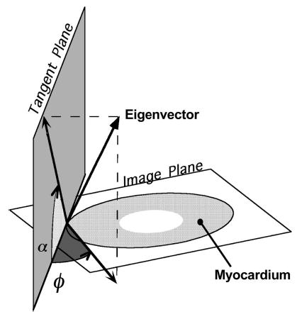
Definition of the two angles are necessary to determine the orientation of the eigenvectors and fibers require first the determination of the tangent plane. At a point on the epicardial surface, this plane is simply the surface tangent plane. For all points along a normal inward from that point, the tangent plane is defined as the plane parallel to the epicardial tangent plane. The inclination angle α is then the angle between the image (horizontal) plane and the projection of the eigenvector (or fiber) onto the tangent plane. The transverse angle φ is defined as the angle between the tangent plane and the projection of the eigenvector onto the image plane.

Comparison of Histological and DTMR Estimates of Orientation Angles in Fixed Myocardium

A transmural plug of tissue with dimensions 8.75×3.5×3.75 mm in the circumferential, longitudinal, and transmural directions, respectively, was removed from the LV free wall of one formaldehyde-fixed heart. The base of the plug was sliced approximately perpendicular to the epicardium. The base of the plug was then placed on a pedestal within the rf coil, and imaged in a plane parallel to the plug base (i.e., the horizontal plane). Imaging was performed with a slice thickness of 2 mm, and with 256 frequency encoding, and 128 phase encoding steps. The readout direction was oriented transmurally, resulting in a resolution through the wall of 156 μm. Diffusion images were obtained as described above—with the exception of four signal averages, rather than 2—and the diffusion tensors and eigenspaces were calculated. Fiber inclination angles were defined as angles from the horizontal (i.e., out of the imaging plane) in a plane tangent to the epicardium. These were tabulated versus percent transmural depth for later comparison with histology.

Following imaging, the plug was paraffin embedded and sectioned. Sections were made serially in a plane parallel to the epicardial surface. Four-μm-thick sections were made every 150 μm beginning at the epicardium and proceeding transmurally. The sections were mounted on slides and stained with hematoxylin and eosin. Sections were photographed at 10× magnification using a digital camera attached to a microscope. Typically, four or five images were taken per section in order to cover its entirety; these images were composited on a computer, resulting in a complete image of the section.

In each histology section, representing a slice of tissue cut parallel to the epicardium (i.e., in a vertical plane), fiber inclination angles were measured relative to the base of the tissue specimen (i.e., the horizontal plane), using NIH Image (version 1.61, Wayne Rasband, National Institutes of Health). Since the horizontal plane was parallel to the imaging plane, inclination angle was defined similarly for both histology and DTMRI—the angle between the horizontal plane and the fibers, in a plane parallel to the epicardium (see Fig. 2).

For each section, five sites spaced by 1.2 mm in the circumferential direction were selected. For each site, up to five measurements of inclination angle were made along the base–apex direction (i.e., along the horizontal line), spanning 2 mm (corresponding to the DTMRI slice thickness). For each of the five sites, the measurements in the base–apex direction were averaged, corresponding to the averaging which occurs in this direction in each voxel due to the 2 mm slice thickness. Thus, one measurement of (base–apex) averaged inclination angle was obtained for each of the five (circumferentially spaced) sites. The procedure was repeated for all slides, each sampling a different transmural depth, and so providing five sets of fiber inclination angle versus section (slide) number. During histological processing, shrinkage of the specimen may occur; therefore, slide numbers were converted to percent transmural depth, enabling appropriate histology and DTMRI measurements to be compared through the wall.

Site 3 for the histology section was chosen to be at the midpoint of the basal edge of the plug at the epicardial surface. To align the DTMRI sites with those of the histological sections, site 3 for the MR image was selected to be at the midpoint of the epicardial edge of the plug. The remaining sites were then spaced as for the histology section. We estimated the uncertainty in the alignment of the sites to be ±500 μm. This is a result of uncertainty in positioning the center of the cutting plane at the midpoint of the basal edge, and selection of the epicardial midpoint on the MR image.

At each of the five sites, and at each transmural depth, histological measurements were compared with DTMRI estimates at the same location. Due to the uncertainty in the placement of the histology sites relative to the MR image in the circumferential direction, we compared each histology measurement: (1) to the average of the DTMRI measurements within ±500 μm in the circumferential direction and at the same transmural depth (referred as the average case); and (2) to the DTMRI measurement within 500 μm to which it was most different (referred to as the the worst case). Correlation coefficients (R) were calculated for these five sets of measurements, as well as the significance of each R. The average rms error for each site was also determined. Finally, the distribution of the differences between the histology and DTMRI measurements was calculated. To detect a systematic error in the measurements, the mean of this distribution was compared to the null hypothesis of zero mean using Student’s t-test, with p<0.05 considered significant.

Reconstruction of Ventricular Geometry and Fiber Orientation

Reconstruction of ventricular anatomy involved three steps. First, epicardial and endocardial boundaries were estimated using both the short-axis GRASS intensity and diffusion-weighted short-axis slices using a semiautomated image segmentation tool called heartworks,²⁸ to be described below. This yielded a series of 128 planar contours defining epicardial and endocardial boundaries. Second, these contours were used to reconstruct the ventricular epicardial and endocardial surfaces for visualization of ventricular structure. Third, diffusion tensor eigenvalues and eigenvectors were computed from the diffusion-weighted short-axis sections coincident with a subset of the GRASS imaging short-axis sections, thus providing estimates of fiber orientation within the myocardium in each of these sections.

heartworks is a software tool developed in the C⁺⁺ programming language for detecting epicardial and endocardial boundaries in each short-axis slice, and for interconnecting these contours in order to visualize cardiac geometry. heartworks implements two distinct methods for semiautomated detection of these boundaries. These are: (a) a parametric active contour method and (b) the method of region growing. The parametric active contour method used is one developed by Xu and Prince.²⁷ In this method, a contour is represented by a parametric function {x(s),y(s)}, where s is normalized arc length along the boundary. Associated with this parametric function is an energy E defined as

$$\begin{array}{l}E=\frac{1}{2}{\int }_0^1\alpha [{x^{\prime }}^2(s)+{y^{\prime }}^2(s)]ds\\ +\frac{1}{2}{\int }_0^1\beta [{x^{″}}^2(s)+{y^{″}}^2(s)]ds\\ +{\int }_0^1{E}_{\text{ext}}(x(s),y(s))ds,\end{array}$$ (3)

where x′(s),y′(s) are first order derivatives of x(s) and y(s), and x″(s) and y″ (s) are second order derivatives of x(s) and y(s) with respect to normalized arc length. The contour is deformed to the boundary by minimizing the energy function E. The first and second integral terms of this energy function are smoothness constraints imposed on the contour. The first term represents the stretching energy of the contour, and the second term corresponds to bending energy. Parameters α and β are weighting factors which influence the contribution of the stretching and bending energy terms to the fit. The third term E_ext is referred to as an external energy function. A formulation of the external function E_ext proposed by Xu and Prince²⁷ is

$$E_{\text{ext}}(x,y)=-|\nabla (G_{\sigma }(x,y)*I(x,y)){|}^2,$$ (4)

where I(x,y) is the gray-scale intensity image, G_σ(x,y) is a 2D Gaussian kernel, * is the convolution operator and ∇ is the gradient operator. These external diffusion forces act to move the contour into boundary concavities.

The concept of region growing, as applied to the computation of epicardial and endocardial boundaries, is to define two distinct regions, R₁ and R₂ , within each GRASS short-axis slice. These regions are: (a) myocardium and either the left or right ventricular cavities (for computation of the endocardial surfaces); or (b) myocardium and the fluid surrounding the heart (for computation of the epicardial boundary). To do this, an initial image pixel is selected within image region R_i (typically the bathing fluid for computation of the epicardial surface or the ventricular cavities for computation of the endocardial surface). This region is then extended in all directions. Let P(R_i) be the probability density of pixel intensities in region R_i , P(g/R_i) be the probability density of pixel intensity g in region R_i , and P(g) be the probability density of pixel intensity g in both regions. Then from Bayes theorem, the probability that a pixel is from region R_i given it’s intensity g is

$$P(R_i|g)=\frac{P(g|R_i)P(R_i)}{P(g)}.$$ (5)

It was assumed that P(g/R_i) is ~N(r,σ), and a pixel is equally likely to be in R₁ or R₂ . Given these assumptions, the region growing algorithm proceeds as follows: (a) choose an initial pixel in R_i ; (b) examine neighboring pixels with intensity g, and compute P(R₁/g) and P(R₂/g); (c) assign each neighboring pixel to a region of maximum likelihood; (d) mark pixels which define a boundary between the two regions; and (e) iterate until all pixels are assigned to a region.

Examples of both segmentation algorithms applied to GRASS images are shown in Fig. 3. Estimated boundaries are shown by the black lines indicated by white arrows. Inspection of Figs. 3(a)–3(b) indicates that both algorithms perform reasonably well in locating the epicardial boundary. However, the method of region growing yields contours better approximating endocardial boundary shape. Use of the method of active contours [Fig. 3(a)] results in a smoothed contour which only approximates detailed structural features seen on the endocardial boundaries. Results obtained using both methods often required editing by the user. For example, the method of region growing was not able to discriminate between myocardium and the imaging artifact seen near the septal-LV–right ventricle (RV) junction of Fig. 3(b). heartworks is therefore equipped with tools for editing (for example, repositioning and locking) contour points and image data.

FIGURE 3.

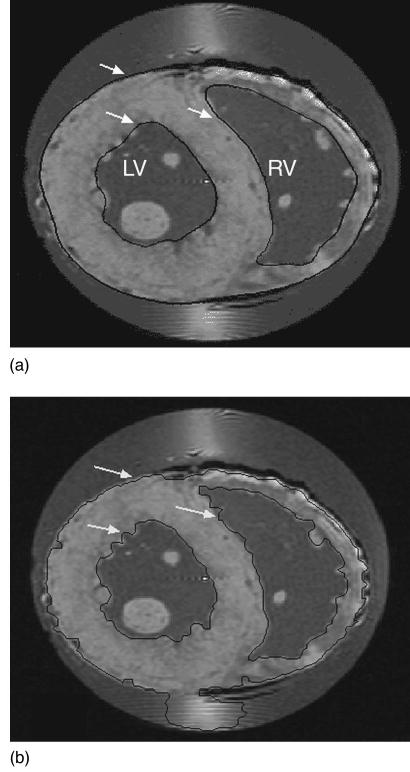
Results of application of the automated boundary finding algorithms available in heartworks to a basal short-axis section through the rabbit heart obtained using GRASS imaging. (A) shows results of application of the active contour method, and (B) results of the region growing method. The black curves bound the epicardium and the endocarium of the LV and RV.

The semiautomated image segmentation algorithms in heartworks provide a set of 3×128 planar contours that specify epicardial and endocardial (RV and LV) surfaces, where each contour is represented by a set of ordered points. Given these contours, ventricular surfaces are reconstructed using a piecewise smooth surface reconstruction algorithm developed by Hoppe and DeRose which determines an optimal triangular tiling between points in adjacent contours.⁶

RESULTS

Comparison of DTMRI and Histology Fiber Orientation

Figure 4(A) shows a color-coded map of fiber inclination angles computed from primary eigenvectors estimated using DTMRI in formaldehyde-fixed rabbit heart. For comparison, inclination angles in a short-axis section of a finite-element model of canine ventricular fiber structure developed by Nielsen et al.¹⁵ are shown in Fig. 4(B). Both show the well-known transmural gradient of fiber inclination angles: negative epicardial angles which become zero near the mid wall, and then positive on the endocardial surfaces of the LV and RV free wall. There is qualitative agreement between these data despite the fact that sections are from different species (rabbit versus canine). This qualitative similarity of transmural variation in fiber angle between species has been reported previously for canine, human, and rabbit ventricular myocardium.^17,24

FIGURE 4.

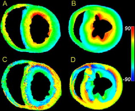
(A) Map of primary eigenvector inclination angle obtained from DTMRI for one slice in a fixed rabbit heart. (B) Fiber inclination angle map obtained from the histological reconstruction of Nielsen et al. for one section of a dog heart. (C) Map of tertiary eigenvector inclination angle obtained from DTMRI for the same slice as in (A). (D) Map of the inclination angles of the laminae normals obtained from the Nielsen et al. reconstruction for the same slice as in (B).

As reported in perfused tissue,¹⁸ the DTMRI data obtained in formaldehyde-fixed myocardium exhibit a systematic pattern of secondary and tertiary eigenvector orientation. Secondary eigenvector orientations point predominantly in the transmural direction. Primary and secondary eigenvectors can therefore be thought of as defining a plane that extends outward from the endocardial surface. The orientation of this plane varies as primary eigenvector orientation rotates with increasing transmural depth. The tertiary eigenvector, by definition, is the local normal to this plane. Figure 4(C) is a color map of the inclination angle of the tertiary diffusion tensor eigenvector in the same short-axis section as shown in Fig. 4(A). Consistent with the general pattern described above, this inclination angle changes from being roughly horizontal at the epicardial surface, to vertical near the mid wall, and approximately horizontal at the endocardial surfaces. The apparent sheet structure formed by the spatial distribution of the tertiary eigenvector is consistent with that of anatomical laminae recently described by LeGrice et al.¹³ in the canine ventricles. For comparison, inclination angles of the laminae normals in a short-axis section of a finite-element model of canine ventricular fiber structure developed by Nielsen et al.¹⁵ are shown in Fig. 4(D). These data show a qualitative correlation between the inclination angles of the diffusion tensor tertiary eigenvector measured in formaldehyde-fixed rabbit heart [Fig. 4(C)], and normal vectors to the laminae measured in canine heart [Fig. 4(D)].

The three-dimensional structure of the diffusion-tensor eigenvectors is explored further in Fig. 5, which show primary [Fig. 5(A)], secondary [Fig. 5(B)], and tertiary [Fig. 5(C)] eigenvectors in a single equatorial short-axis section. Line segments are used to display the three-dimensional orientation of each eigenvector. Orientation of the segment with respect to the plane of section is also represented using the indicated color code. Red represents vectors whose fractional out-of-plane component approaches unity, whereas blue represents vectors with zero out-of-plane component (i.e., vectors that lie in the plane of section). Primary eigenvectors [Fig. 5(A)] display a clear transmural rotation. That is, these vectors exhibit a significant vertical (long-axis) component on the epicardial and endocardial surfaces denoted by the yellow and red colors, and rotate to become horizontal (blue) in the mid wall.

FIGURE 5.

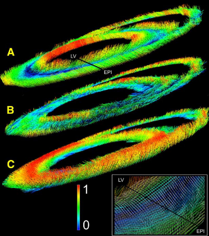
Distribution of primary (A), secondary (B), and tertiary (C) eigenvectors within an equatorial short-axis cross section. Orientation of the line segments indicates eigenvector orientation. The normalized out-of-plane component of each vector is shown according to the indicated color code.

As noted previously, secondary eigenvectors within the LV and septal myocardium [Fig. 5(B)] exhibit a transmural orientation, and lie largely within the horizontal plane. This can be seen by the blue and green color coding of many of the segments. Their orientation is more complex within the RV myocardium, with vertical vectors being more common. The inset magnifies the area around the black transmural line extending from the LV to the epicardium (labeled EPI) in Fig. 5(A). Secondary eigenvectors are shown as white line segments overlying the colored primary eigenvectors. The predominant transmural orientation of the secondary eigenvectors can be seen in this figure, as can the predominantly circumferential orientation of primary eigenvectors.

A transmural gradient is also seen for the tertiary eigenvectors [Fig. 5(C)], especially in the septal and LV myocardium. Since this eigenvector is by definition orthogonal to the plane formed by primary and secondary eigenvectors at each point, tertiary eigenvectors are oriented vertically (red) where the primary and secondary are horizontal (blue). Further, as the secondary eigenvector has a predominant radial orientation, tertiary eigenvectors tend to lie within the circumferential–longitudinal plane. The structure in the RV myocardium is again more complex, with some of the tertiary eigenvectors taking on a radial organization (see the green vectors on the RV free wall endocardium).

Previously, we have reported a close correspondence between fiber angle measured using histological methods, and inclination angle of the primary diffusion tensor measured at the same tissue locations using DTMRI applied to perfused tissue.¹⁸ Quantitative comparison of histological and DTMRI-based estimates of inclination angle measured in formaldehyde-fixed tissue show an even closer correspondence.⁵ An example of this is shown in Fig. 6(A), in which inclination angle determined by histology (open circles) and using DTMRI (filled circles) are shown at one of five sites on a fixed rabbit heart. Correlation coefficients were 0.979 (average case) and 0.966 (worst case), all with a significance level of p<0.001. The average Pearson correlation coefficient between histological and DTMRI estimates from perfused myocardium is 0.86.¹⁸ Close correspondence is further supported by comparing each histology measurement with the DTMRI estimate at the same percent transmural distance for that site. This provides an average rms error of 5.3° and standard deviation (s.d.) of 5.1° for the average case, and 10.3 (average), 7.4 (s.d.) for the worst case (N=70 for both).

FIGURE 6.

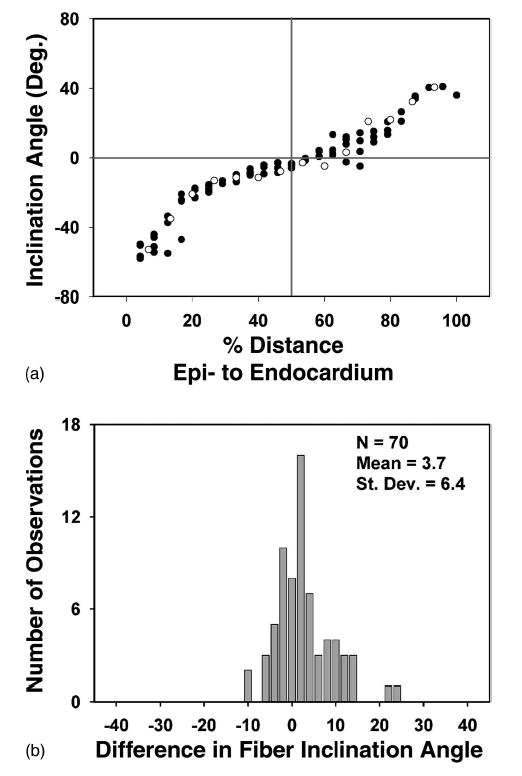
(A) Fiber inclination angle measured histologically (open circles) and primary eigenvector inclination angle estimated using DTMRI (filled circles) obtained from a fast spin-echo pulse sequence for site 1 of the tissue plug. (B) Distribution of differences in fiber inclination angle at each voxel obtained using histology (α_hist) and DTMRI (α_mri).

The correspondence of the histology and DTMRI measurements are further quantified in Fig. 6(B), where the differences between the histology and averaged DTMRI values for all sites are shown (average case). The mean of this distribution represents the degree of systematic error (i.e., degree of constant shift of one set of measurements relative to the other) present. The positive mean of 3.7° is significantly different from zero (SE=0.76, p<0.001). The distribution median is 3.5°, and the distribution s.d. of 6.4° is of course similar to the s.d. of the rms error (with equality achieved only for a symmetric distribution). The maximum error is 24.3°, while over 82% of the errors fall between −10° and 10°. If the worst case is instead considered, the s.d. of the distribution increases to 7.9°.

A second angle in addition to the inclination angle is required to fully specify the position of an eigenvector or fiber in three dimensions. Previous histological measurements of fiber orientation have found this angle to be small, suggesting that the fibers lie primarily in planes parallel to the epicardium. The average value for the plug was 4.6°±3.4°, similar to previous histological measures of this angle in dog myocardium of 4.6°±0.76° and 7.3°±0.9°.^20,21

Ventricular Reconstructions

Figure 7(A) shows reconstruction of a rabbit ventricle based on GRASS image data obtained at a spatial resolution of 156×312×469 μm. Image segmentation was performed using the method of active contours. Papillary muscles projecting into the ventricles were edited from the images using heartworks. LV and RV surfaces are shown in gold and red, respectively. The epicardial surface is rendered as a wire frame mesh. The high spatial resolution afforded by GRASS imaging is sufficient to reveal the highly detailed structure of both the epicardial and endocardial surfaces.

FIGURE 7.

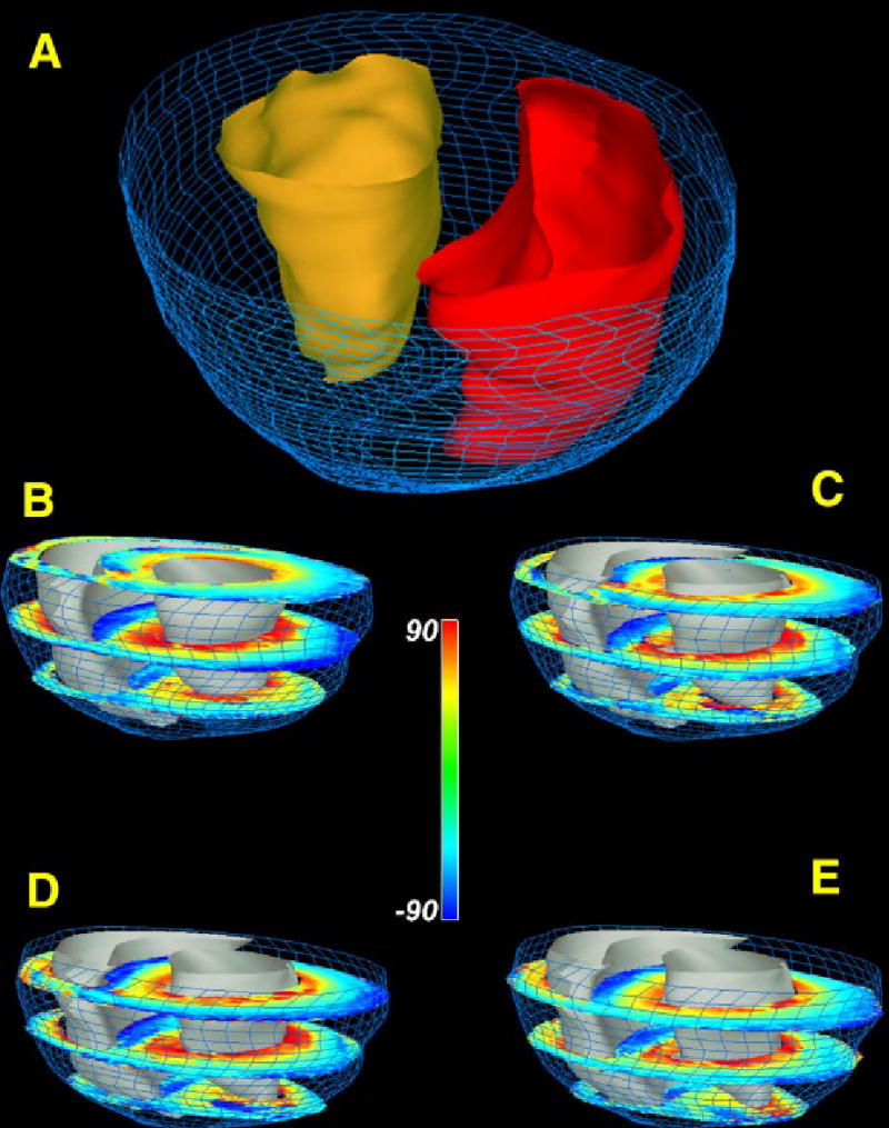
(A) Reconstruction of epicardial (blue wire mesh) and endocardial surfaces (RV endocardium—red; LV endocardium—gold). (B)–(E) Short-axis sections of rabbit ventricular myocardium in which fiber inclination angle is color coded. Short-axis section numbers, beginning from the most basal section, are: 1,7,13 (B); 2,8,14 (C); 3,9,15 (D); 4,10,16 (E).

Figures 7(B)–7(E) shows the reconstructed ventricle of Fig. 7(A) into which 12 of 20 short-axis DTMRI sections are inserted. Each of these sections shows fiber inclination angle coded according to the indicated color map. In general, these sections show a transmural variation in fiber angle from the epicardial to endocardial surfaces. As described in Nielsen et al.¹⁵ there are sharp transitions in fiber orientation in the mid wall near the RV–septal junctions.

DISCUSSION

We have reported previously that DTMRI can be used to estimate, with a high degree of accuracy, fiber orientation in either perfused¹⁸ or fixed⁵ ventricular myocardium. The results reported here demonstrate that DTMRI of fixed myocardium can be used to reconstruct the three-dimensional fiber organization of ventricular myocardium.

There are several advantages afforded by use of DT-MRI for ventricular reconstruction. First, by removing data corruption due to heart motion, fixation enables longer imaging times resulting in higher spatial resolution than available when imaging the perfused heart. As one measure of this higher spatial resolution, the ventricular reconstruction reported here is based on estimates of the diffusion tensor eigensystem at 196,867 myocardial points in the rabbit heart. This stands in contrast to roughly 14,300 measurement points of fiber orientation reported previously for rabbit heart,²⁵ and roughly 17,000 points in canine myocardium.¹⁰ The absence of perfusion also eliminates potential flow artifacts. DTMRI in fixed tissue can also be performed at elevated temperatures, thus increasing water diffusivity and therefore diffusion anisotropy. Second, the imaging time required for the reconstructions reported here (~20 h) is significantly less than that required to perform direct anatomical reconstruction—a procedure requiring many days of efforts. Image acquisition can also be automated through software controlled scanner operation. These relatively short imaging and reconstruction times should make possible the acquisition of an extensive library of reconstructed hearts in both normal and disease states. Third, DTMRI yields the absolute orientation of all three diffusion tensor eigenvectors at each imaged material point. Histological reconstruction methods at best provide estimates of the angles defining either fiber or sheet orientation at nearby, but not identical, measurement points.

The qualitative agreement between inclination angle of the diffusion tensor tertiary eigenvector in rabbit [Fig. 4(C)] and inclination angle of the surface normal to myocardial sheets measured in canine myocardium [Fig. 4(D)] suggests that DTMRI may also be used to reconstruct the laminar structure of the heart. This hypothesis is supported further by the data shown in the inset of Fig. 5, which demonstrate the predominant transmural orientation of the secondary diffusion tensor eigenvector. We have conjectured previously as to possible anatomical origins for the correlation between the tertiary eigenvector and the sheet normal.¹⁸ However, confirmation of this hypothesized correlation awaits histological reconstruction of sheet structure in a heart reconstructed using DTMRI.

Finally, in this study we have made no attempt to represent the spatial complexity of the cardiac ventricular fiber field using finite-element models—work which has been pioneered by researchers at Auckland University.^{8–10,13–15} and UCSD.²⁴ As with anatomical data, such models would provide efficient representations of the wealth of structural data now available using diffusion-tensor MR imaing in fixed myocardium.

References

- 1.Atalay MK, Reeder SB, Zerhouni EA, Forder JR. Blood oxygenation dependence of T1 and T2 in the isolated, perfused rabbit heart at 4.7T. Magn Reson Med. 1995;34:623–627. doi: 10.1002/mrm.1910340420. [DOI] [PubMed] [Google Scholar]
- 2.Basser PJ, Mattiello J, LeBihan D. Estimation of the effective self-diffusion tensor from the NMR spin echo. J Magn Reson, Ser B. 1994;103:247–254. doi: 10.1006/jmrb.1994.1037. [DOI] [PubMed] [Google Scholar]
- 3.Chatham JC, Ackerman S, Blackband SJ. High-resolution 1H NMR imaging of regional ischemia in the isolated perfused rabbit heart at 4.7 T. Magn Reson Med. 1991;21:144–150. doi: 10.1002/mrm.1910210118. [DOI] [PubMed] [Google Scholar]
- 4.Chen PS, Cha YM, Peters BB, Chen LS. Effects of myocardial fiber orientation on the electrical induction of ventricular fibrillation. Am J Physiol. 1993;264:H1760–H1773. doi: 10.1152/ajpheart.1993.264.6.H1760. [DOI] [PubMed] [Google Scholar]
- 5.Holmes AA, Scollan DF, Winslow RL. Direct histological validation of diffusion tensor MRI in formaldehyde-fixed myocardium. Magn Reson Med. 2000;44:157–161. doi: 10.1002/1522-2594(200007)44:1<157::aid-mrm22>3.0.co;2-f. [DOI] [PubMed] [Google Scholar]
- 6.Hoppe H, DeRose T, DuChamp T, McDonald J, Stuetzle W. Piecewise smooth surface reconstruction from unorganized points. Comput Graph. 1992;26(2):71–78. [Google Scholar]
- 7.Hsu EW, Muzikant AL, Matulevicius SA, Penland RC, Henriquez CS. Magnetic resonance myocardial fiber-orientation mapping with direct histological correlation. Am J Physiol. 1998;274:H1627–H1634. doi: 10.1152/ajpheart.1998.274.5.H1627. [DOI] [PubMed] [Google Scholar]
- 8.Hunter PJ. Proceedings: Development of a mathematical model of the left ventricle. J Physiol (London) 1974;241:87P–88P. [PubMed] [Google Scholar]
- 9.Hunter PJ, Smaill BH. The analysis of cardiac function: a continuum approach. Prog Biophys Mol Biol. 1988;52:101–164. doi: 10.1016/0079-6107(88)90004-1. [DOI] [PubMed] [Google Scholar]
- 10.Hunter PJ, Nielsen PM, Smaill BH, LeGrice IJ, Hunter IW. An anatomical heart model with applications to myocardial activation and ventricular mechanics. Crit Rev Biomed Eng. 1992;20:403–426. [PubMed] [Google Scholar]
- 11.Kanai A, Salama G. Optical mapping reveals that re-polarization spreads anisotropically and is guided by fiber orientation in guinea pig hearts. Circ Res. 1995;77:784–802. doi: 10.1161/01.res.77.4.784. [DOI] [PubMed] [Google Scholar]
- 12.Koide T, Narita T, Sumino S. Hypertrophic cardiomyopathy without asymmetric hypertrophy. Br Heart J. 1982;47:507–510. doi: 10.1136/hrt.47.5.507. [DOI] [PMC free article] [PubMed] [Google Scholar]
- 13.LeGrice IJ, Hunter PJ, Smaill BH. Laminar structure of the heart: a mathematical model. Am J Physiol. 1997;272:H2466–H2476. doi: 10.1152/ajpheart.1997.272.5.H2466. [DOI] [PubMed] [Google Scholar]
- 14.LeGrice IJ, Smaill BH, Chai LZ, Edgar SG, Gavin JB, Hunter PJ. Laminar structure of the heart: ventricular myocyte arrangement and connective tissue architecture in the dog. Am J Physiol. 1995;269(2Pt2):H571–H582. doi: 10.1152/ajpheart.1995.269.2.H571. [DOI] [PubMed] [Google Scholar]
- 15.Nielsen PM, I, Le Grice J, Smaill BH, Hunter PJ. Mathematical model of geometry and fibrous structure of the heart. Am J Physiol. 1991;260:H1365–H1378. doi: 10.1152/ajpheart.1991.260.4.H1365. [DOI] [PubMed] [Google Scholar]
- 16.Reeder SB, Atalay MK, McVeigh ER, Zerhouni EA, Forder JR. Quantitative cardiac perfusion: a noninvasive spin-labeling method that exploits coronary vessel geometry. Radiology. 1996;200:177–184. doi: 10.1148/radiology.200.1.8657907. [DOI] [PMC free article] [PubMed] [Google Scholar]
- 17.Reese TG, Weisskoff RM, Smith RN, Rosen BR, Dinsmore RE, Wedeen VJ. Imaging myocardial fiber architecture in vivo with magnetic resonance. Magn Reson Med. 1995;34:786–791. doi: 10.1002/mrm.1910340603. [DOI] [PubMed] [Google Scholar]
- 18.Scollan D, Holmes A, Winslow RL, Forder J. Histological validation of myocardial microstructure obtained from diffusion tensor magnetic resonance imaging. Am J Physiol. 1998;275(44):H2308–H2318. doi: 10.1152/ajpheart.1998.275.6.H2308. [DOI] [PubMed] [Google Scholar]
- 19.Stejskal EO, Tanner JE. Spin diffusion measurements: spin echoes in the presence of time-dependent field gradient. J Chem Phys. 1965;42:288–292. [Google Scholar]
- 20.Streeter, D. Gross morphology and fiber geometry of the heart. In: Handbook of Physiology, The Cardiovascular System I, edited by R. Berne, Bethesda, MD: American Physiological Society, 1979, Chap. 4, pp. 61–112.
- 21.Streeter, D., W. Powers, M. Ross, and F. Torrent-Guasp. Three dimensional fiber orientation in the mammalian left ventricular wall. In: Cardiovascular Systems Dynamics, edited by J. Bann, A. Noordegraaf, and J. Raines, Cambridge, MA: MIT Press, 1979, Chap. 9, pp. 73–84.
- 22.Streeter D, Spotnitz H, Patel D, Ross J, Sonnenblick E. Fiber orientation in the canine left ventricle during diastole and systole. Circ Res. 1969;24:339–347. doi: 10.1161/01.res.24.3.339. [DOI] [PubMed] [Google Scholar]
- 23.Thickman DI, Kundel HL, Wolf G. Nuclear magnetic resonance characteristics of fresh and fixed tissue: the effect of elapsed time. Radiology. 1983;148:183–185. doi: 10.1148/radiology.148.1.6856832. [DOI] [PubMed] [Google Scholar]
- 24.Vetter FJ, McCulloch AD. Three-dimensional analysis of regional cardiac function: a model of rabbit ventricular anatomy. Prog Biophys Mol Biol. 1998;69:157–183. doi: 10.1016/s0079-6107(98)00006-6. [DOI] [PubMed] [Google Scholar]
- 25.Waldman LK, Nosan D, Villarreal F, Covell JW. Relation between transmural deformation and local myofiber direction in canine left ventricle. Circ Res. 1988;63:550–562. doi: 10.1161/01.res.63.3.550. [DOI] [PubMed] [Google Scholar]
- 26.Wickline SA, Verdonk ED, Wong AK, Shepard RK, Miller JG. Structural remodeling of human myocardial tissue after infarction Quantification with ultrasonic backscatter. Circulation. 1992;85:259–268. doi: 10.1161/01.cir.85.1.259. [DOI] [PubMed] [Google Scholar]
- 27.Xu C, Prince JL. Snakes, shapes and gradient vector flow. IEEE Trans Image Process. 1995;7:359–369. doi: 10.1109/83.661186. [DOI] [PubMed] [Google Scholar]
- 28.Zhang, J. MR-based reconstruction of cardiac geometry, MS thesis, The Johns Hopkins University, Biomedical Engineering, Baltimore, 1999.