Efficient Study Designs for Test of Genetic Association Using Sibship Data and Unrelated Cases and Controls

Abstract

Linkage mapping of complex diseases is often followed by association studies between phenotypes and marker genotypes through use of case-control or family-based designs. Given fixed genotyping resources, it is important to know which study designs are the most efficient. To address this problem, we extended the likelihood-based method of Li et al., which assesses whether there is linkage disequilibrium between a disease locus and a SNP, to accommodate sibships of arbitrary size and disease-phenotype configuration. A key advantage of our method is the ability to combine data from different family structures. We consider scenarios for which genotypes are available for unrelated cases, affected sib pairs (ASPs), or only one sibling per ASP. We construct designs that use cases only and others that use unaffected siblings or unrelated unaffected individuals as controls. Different combinations of cases and controls result in seven study designs. We compare the efficiency of these designs when the number of individuals to be genotyped is fixed. Our results suggest that (1) when the disease is influenced by a single gene, the one sibling per ASP–control design is the most efficient, followed by the ASP-control design, and familial cases contribute more association information than singleton cases; (2) when the disease is influenced by multiple genes, familial cases provide more association information than singleton cases, unless the effect of the locus being tested is much smaller than at least one other untested disease locus; and (3) the case-control design can be useful for detecting genes with small effect in the presence of genes with much larger effect. Our findings will be helpful for researchers designing and analyzing complex disease-association studies and will facilitate genotyping resource allocation.

Association analysis provides a powerful tool for identifying genetic variants that predispose to complex diseases. Association analysis with use of genetic markers (such as SNPs) relies on the presence of linkage disequilibrium (LD), which occurs when specific alleles at the disease and marker loci appear together in gametes more frequently than expected by chance. With the recent availability of high-throughput SNP genotyping and decreasing genotyping costs, association studies with use of SNPs are beginning to be conducted genomewide.^1,2 Such analyses have been facilitated by progress on the International HapMap Project,^3,4 which cataloged and genotyped millions of SNPs, allowing informative tagging SNPs to be selected for different populations. Genomewide association studies typically involve hundreds or thousands of individuals and, since genotyping on such a large scale is still expensive, it is important to choose efficient study designs.

In gene-mapping studies, affected sib pairs (ASPs) or multiplex affected sibships are often collected for linkage analyses. Although these individuals may be reused in follow-up association studies, this is not always done. Traditionally, association-mapping studies with the case-control design have been used to test for disease-marker association by selecting one affected sibling per sibship, to form the case group, and comparing the alleles or genotype frequencies with a random sample of unaffected individuals. It has been shown that power can be substantially increased by including families with more affected siblings^5–7 in association studies. The increase of power is due to the enrichment of disease-predisposing alleles in affected sibships; this, in turn, leads to improved power to detect genetic association because of larger allele-frequency differences between cases and controls.

Efficient use of data sets that include related individuals in association studies requires a unified statistical framework that allows the joint analysis of all available sampling units. In this article, we extend the association test proposed by Li et al.⁸ to the analysis of sibships of arbitrary size and disease-phenotype configuration and to accommodate parental genotypes, when available. Our method allows the analysis of data containing mixed types of sampling units that are based on a unified retrospective likelihood framework and therefore can evaluate evidence of disease-marker association on the basis of different sampling units, ranging from unselected unrelated individuals to large sibships. We consider scenarios for which genotypes are available for unrelated cases, ASPs, or only one sibling per ASP. We construct designs that use affected individuals only and others that use unaffected siblings or unrelated unaffected individuals as controls. Using our unified likelihood framework, we compare efficiency of these study designs when the number of individuals to be genotyped is fixed.

As noted elsewhere by Risch,⁶ we show that designs with unrelated controls are more powerful than are designs with family-based controls. Our results also suggest that, for diseases that are influenced by multiple genes, familial cases provide more association information than do singleton cases, unless the effect of the test locus is much smaller than at least one other untested disease locus. Similar phenomena have been observed by Risch⁹ for single major-locus models with an additive polygenic background and by Howson et al.¹⁰ for certain two-locus models. Further, we show that the case-control design can be useful for detecting genes with small effect in the presence of genes with much larger effect.

Methods

We consider the problem of disease-marker association analysis with mixed types of sampling units. Our goals are to develop a unified likelihood framework that allows the joint analysis of all available data and to compare efficiency of different study designs for testing association between disease and a candidate SNP, given fixed genotyping resources. We discuss the impact of phenotyping cost in the “Discussion” section.

Assumptions and Definitions

We assume there is a set of sibships genotyped at a candidate SNP and, optionally, M⩾0 flanking markers. We assume the SNP, with alleles A and a (with frequencies p_A and p_a), is completely linked (recombination fraction θ=0) to a diallelic disease locus, with disease-predisposing allele D and alternate allele d (with frequencies p_D and p_d). We wish to evaluate evidence of association at the candidate SNP by modeling the disease-SNP haplotypes DA, Da, dA, and da (with frequencies p_DA, p_Da, p_dA, and p_da, respectively) and the penetrances f_g=P(affected|g) for disease genotypes g∈{dd, Dd, DD}. As shown later, unrelated individuals do not allow the estimation of all these independent parameters. In samples that include only unrelated individuals, we assume that the disease and SNP loci are in complete LD (r²=1), so that their allele frequencies are identical. The assumption that r²=1 results in an identifiable model but no loss of statistical efficiency, since we can still extract maximum information from the available data.

By definition, the population prevalence of the disease K=f_ddp²_d+2f_Ddp_dp_D+f_DDp²_D, and the genotype relative risk (GRR)=f_g/f_dd for g∈{Dd,DD}. We allow LD between the candidate SNP and the unobserved disease alleles but assume linkage equilibrium between the flanking markers and the superlocus formed by combining the disease and SNP loci. We assume Hardy-Weinberg equilibrium in the general population for all markers, including the superlocus. We further assume that the disease phenotypes of the siblings are independent, given their genotypes at the disease locus, and that there is a single disease causal variant in the region. We investigate the impact of multiple disease variants in the “Simulations” section.

For a sibship with s siblings, let

be the observed unordered marker genotypes, Y be the disease phenotypes, and G be the disease-SNP haplo-genotypes. Let θ_m be the recombination fraction between markers m and m+1 (1⩽m⩽M-1). The inheritance pattern at marker m is completely described by a binary inheritance vector v_m of length 2s,^11,12 whose entries indicate the outcome of the paternal and maternal meioses for the s siblings in the sibship. Let v_D and v_SNP denote the inheritance vectors at the disease locus and the candidate SNP, respectively. Complete linkage between the disease and SNP loci implies v_D≡v_SNP. For ease of computation, we assume there is no genetic interference, so that {v_m} forms a hidden Markov chain.

Conditional Probability of Marker Data, Given Disease Phenotypes for a Sibship with s Siblings

We wish to evaluate P(X|Y), the conditional probability of marker genotypes X, given disease phenotypes Y for a sibship with s siblings. By the law of the total probability,

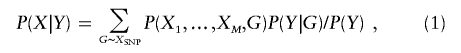where the summation is taken over all disease-SNP haplogenotypes that are consistent with the observed SNP genotypes. Summing over all possible inheritance vectors at the disease locus and applying Baum’s¹³ forward and backward algorithms,

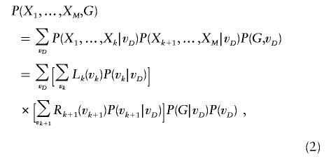where k and k+1 are flanking markers on the left and right side of the candidate SNP. The summation over all possible inheritance vectors allows the handling of incomplete inheritance information and phase ambiguity by incorporating prior probabilities of the inheritance vectors. At any marker m(1⩽m⩽M),

and

The calculation of equation (2) requires three probabilities: (1) the prior probability of inheritance vector v_D, (2) the inheritance vector transition probability between two consecutive markers, and (3) the conditional probability of marker genotypes, given the inheritance vector at that marker. Clearly, the prior probability P(v_D)=2^-2s.

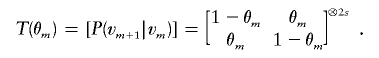
The transition probability between inheritance vectors at markers m and m+1 can be obtained from the transition matrix, which is expressed as the Kronecker power of 2×2 transition matrices corresponding to transitions at each of the 2s meioses,

For example, for a sib pair,

and

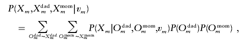
Let O^dad_m and O^mom_m represent the ordered genotypes of the father and the mother at marker m. In ordered genotypes, the maternal allele always precedes the paternal allele. Although observed genotypes are typically unordered, summing over ordered genotypes is computationally convenient, because, taken together, ordered genotypes for the founders and the inheritance vector specify the genotypes of all individuals in the pedigree. Thus, the conditional probability of sibship genotype X_m, given inheritance vector v_m, can be calculated as

where P(X_m|O^dad_m,O^mom_m,v_m) takes the value of 1 if the sibship’s genotype data X_m are consistent with the ordered parental genotypes O^dad_m and O^mom_m and the inheritance vector v_m, and 0 otherwise. The summation is taken over all ordered parental genotypes. P(G|v_G) can be calculated in a similar fashion, by regarding each haplogenotype as a genotype of the superlocus formed by combining the disease and SNP loci.

Recursive calculation of L_m(v_m) and R_m(v_m) with use of these three probabilities allows equation (2) to be evaluated in a manner linear in the number of marker loci M. Equation (2) is an extension of the retrospective likelihood calculation for ASPs described by Li et al.⁸ Here, the sibship size can be >2, and siblings can be either affected or unaffected. Our likelihood calculation easily allows for missing genotypes. For example, to accommodate sibships in which only a subset of the siblings is genotyped at the candidate SNP, we sum over all possible SNP genotypes for those siblings of known disease status but with missing SNP genotypes. It is essential to include all these members, because siblings with known phenotypes but missing genotypes contribute association information.

Our calculation can be readily extended to accommodate parental genotypes. Following the derivation of equation (2), the critical part in the calculation is the conditional probability of marker genotypes for the siblings and their parents, given the inheritance vector at a particular marker. Let X^dad_m and X^mom_m represent the observed unordered parental genotypes at marker m. Then the conditional probability of the observed genotypes given the inheritance vector at marker m is

where the summation is taken over all ordered parental genotypes that are consistent with the observed unordered parental genotypes. This extension enables us to analyze nuclear families with genotyped parents, including parent-affected offspring trios, which are the basic sampling units used by the transmission/disequilibrium test.¹⁴

Under the assumption that the disease phenotypes are independent given the genotypes at the disease locus, P(Y|G) is the product of simple functions of penetrances. An affected sibling j (1⩽j⩽s) with disease-SNP haplo-genotype G_j contributes a term f_Gj, and an unaffected sibling j contributes a term 1-f_Gj. By the law of the total probability, the probability of the disease phenotypes for the sibship

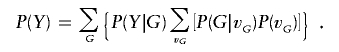Substituting equation (2), P(Y|G), and P(Y) into equation (1), we obtain the conditional probability for the sibship P(X|Y) as a function of model parameters {f_dd,f_Dd,f_DD,p_DA,p_Da,p_dA}.

In the calculation of P(Y|G) and P(Y), we assume that the disease statuses of the siblings are conditionally independent, given their genotypes at the disease locus. This assumption is exactly true only when there are no other genetic or environmental risk factors shared among the siblings. If the disease is influenced by multiple disease variants, then the calculation will depend on genotypes at the other disease loci as well. For example, if the disease is influenced by two unlinked disease loci, then

where subscripts 1 and 2 denote the two unlinked disease loci.

Conditional Probability of Marker Data, Given Disease Phenotype for a Single Individual

In principle, equation (1) can be applied to singleton individuals who can be regarded as sibships with one sibling. However, data sets containing solely unrelated individuals do not allow the estimation of all our model parameters. In this case, we assume that the disease and SNP loci are in complete LD, so that p_D=p_A, and we reparameterize our model. For case-control data,

which is a function of {f_dd,f_Dd,f_DD,p_A}. For a sample of unrelated cases, P(X_SNP|Y) is simply a function of the two SNP genotype frequencies, P(AA|case) and P(Aa|case). For studies that involve only unrelated individuals, flanking markers do not contribute information on association; therefore, we need to consider only the SNP genotypes. It is worth noting that, for SNPs that are in incomplete LD with the disease locus, the genetic effect will be underestimated; however, there is no loss of efficiency for the association test.

Pooling across Different Sampling Units

A key advantage of our likelihood calculation is that it allows the joint analysis of different sampling units in a unified statistical framework, which leads to more efficient use of the available data. The retrospective likelihood for data that contain N independent sibships, which may be of different sizes and disease phenotype configurations, is

Here, we choose to use a retrospective likelihood, since the sibships are ascertained through disease status. Using a retrospective likelihood avoids the problem of ascertainment bias and provides parameter estimates that are valid for the general population.^15,16 In addition, it ensures that our test remains valid even if there are additional genetic or environmental factors that induce correlation between family members.

Test of Association

We wish to evaluate whether a SNP is associated with the putative disease locus. Under the null hypothesis of no association, the SNP and the disease locus are in linkage equilibrium, and the disease-SNP haplotype frequencies are the product of the corresponding disease and SNP allele frequencies (for example, p_DA=p_Dp_A). In this case, parameters that need to be estimated are {f_dd,f_Dd,f_DD,p_D,p_A}, and we set

Under the alternative hypothesis, we maximize a total of six parameters {f_dd,f_Dd,f_DD,p_DA,p_Da,p_dA}. For data including only ASPs or only unrelated individuals, these parameters are not all identifiable, and we reparameterize the likelihood as described by Li et al.⁸ or maximize a subset of the parameters as detailed in table 1. We perform this maximization using a simplex algorithm,¹⁷ an optimization method that does not require derivatives.

Table 1.

Parameters and Constraints for Different Sampling Units^[Note]

	General Model (0⩽r2⩽1)		Linkage Equilibrium Model (r2=0)
Sampling Units	Parameters	Constraints	Parameters	Constraints
Sibship (s⩾3 or mixed sampling units)	{fdd,fDd,fDD,pDA,pDa,pdA}	0⩽fdd,fDd,fDD⩽1; 0⩽pDA,pDa,pdA⩽1; 0⩽pDA+pDa+pdA⩽1	{fdd,fDd,fDD,pD,pA}	0⩽fdd,fDd,fDD⩽1; 0<pD,pA<1
Sib pair (s=2)	{fdd,fDd,fDD,pDA,pDa,pdA}	0⩽fdd,fDd,fDD⩽1; 0⩽pDA,pDa,pdA⩽1; 0⩽pDA+pDa+pdA⩽1	{z0,z1,pA}	0⩽z1⩽0.5,0⩽z0⩽0.5z1 (ASP); 0.5⩽z1⩽2z0,0⩽z0+ z1⩽1 (DSP); 0<pA<1
Case-control	{fdd,fDd,fDD,pA}	0⩽fdd,fDd,fDD⩽1; 0<pA<1	{pA}	0<pA<1
Case only	{P(AA|case),P(Aa|case)}	0⩽P(AA|case),P(Aa|case)⩽1; 0<P(AA|case)+P(Aa|case)<1	{pA}	0<pA<1

Note.— Disease penetrances f_dd, f_Dd, and f_DD are assumed to be not all equal. z_i,i=0, 1, 2, is the probability of sharing i alleles identical by decent for a sib pair.

Following Li et al.,⁸ we use a likelihood-ratio statistic to test for association. We compare the likelihood maximized under the general model (0⩽r²⩽1), , with the likelihood maximized under the null model (r²=0), , using the likelihood-ratio statistic . Parameters associated with each model for the different sampling units and the corresponding parameter constraints are summarized in table 1. For data sets that contain only unrelated cases and controls, our association test is similar to the unconstrained genotype test proposed by Thompson et al.,¹⁸ except that we do not assume known disease prevalence. Our test is also similar to the goodness-of-fit test proposed by Wittke-Thompson et al.¹⁹

In principle, the asymptotic distribution of T_LE under the null hypothesis can be approximated by mixture of χ² distributions,²⁰ but we have not derived the degrees of freedom and mixing parameters because of the complexity of parameter constraints and boundaries. Instead, we assess significance of the test statistic empirically by simulating marker genotypes under the null hypothesis and comparing the observed statistic with the simulated null distribution.

Under the null hypothesis, we sample SNP genotypes for a sibship conditional on their observed flanking-marker genotypes and parameter estimates for the linkage equilibrium model. We leave flanking-marker genotypes unchanged from their observed values. For a single individual, we sample the SNP genotype according to the estimated SNP genotype frequencies. The null distribution of T_LE can be obtained by calculating the statistic for a large number of simulated data sets.

Study Designs for Test of Genetic Association

Our likelihood calculation allows the analysis of sibships of arbitrary size and disease-phenotype configuration, including unrelated affected or unaffected individuals, ASPs, and discordant sib pairs (DSPs). For ease of presentation, we consider only sibships of size ⩽2. To construct different study designs, we select either (1) one or two cases from each ASP or (2) unrelated affected individuals. We use either cases only or select controls from unrelated unaffected individuals or unaffected siblings. Different combinations of cases and controls result in seven study designs (fig. 1). It is worth noting that both the one sibling per ASP–control design and the case-control design use unrelated affected and unaffected individuals. The difference is that, for the one sibling per ASP–control design, the cases are selected from ASPs, whereas, in the case-control design, the cases are randomly selected from the general population.

Figure 1.

Association study designs. The black arrows denote individuals to be genotyped at the candidate SNP. The number of individuals to be genotyped at the SNP is fixed at 1,000 for each study design.

Given fixed genotyping resources, it is important to know which study designs are the most powerful for detecting disease-SNP association. Since disease-mapping studies often start from linkage analysis and since flanking-marker genotypes often are already available, for these studies, we compare the efficiency of different study designs by fixing the total number of individuals to be genotyped at the candidate SNP, and we do not account for the cost or effort associated with collecting flanking-marker data.

Simulations

We performed a set of simulations to evaluate the efficiency of different study designs and to compare the statistical power of our test with other existing association tests. Table 2 describes the single-locus disease models that we considered, which varied over a range of attributable fractions, disease allele frequencies, and GRRs. We set the locus-specific sibling recurrence risk ratio λ_s²¹ to 1.02.

Table 2.

Characteristics of the Simulated Single-Locus Disease Models When λ_s=1.02^[Note]

Model and fdd	fDD	pD	AFa	GRRb
Dominant:
.045	.071	.1	.098	1.57
.039	.060	.3	.214	1.53
.031	.056	.5	.380	1.82
.013	.054	.7	.744	4.19
Recessive:
.049	.179	.1	.026	3.68
.046	.087	.3	.074	1.88
.044	.069	.5	.126	1.58
.040	.061	.7	.205	1.53
Additive:
.045	.092	.1	.094	1.52, 2.04
.041	.072	.3	.186	1.38, 1.76
.036	.064	.5	.282	1.39, 1.79
.028	.059	.7	.430	1.54, 2.09

Note.— Population disease prevalence K was fixed at 5%.

^aAF = attributable fraction.

^bGRR=f_g/f_dd for g∈{Dd,DD}.

When simulating the data, we assumed that the disease and SNP allele frequencies are identical, in contrast to our model in which these frequencies are allowed to differ. Setting these frequencies to be equal allowed us to compare the efficiency of different study designs over a broad range of LD (0⩽r²⩽1) between the disease alleles and the SNP. We assumed a map of 10 markers, each with four equally frequent alleles (heterozygosity H=0.75) evenly spaced at 11.16-cM intervals, corresponding to θ=0.1 under Haldane’s²² no-interference map function. We centered the disease locus and candidate SNP in the middle of the map and assumed zero recombination between them. The disease locus genotypes were removed prior to data analysis. For each of the disease models in table 2, we simulated 5,000 replicate data sets for each design under linkage equilibrium, to estimate the null distribution. We next simulated 2,000 replicate data sets with various levels of LD, to assess the empirical power of our association test.

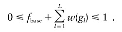
To examine the impact of multilocus inheritance on the relative efficiency of the case-control design and the one sibling per ASP–control design, we also simulated data sets using the additive multilocus disease models for which the multilocus penetrance is the total of the penetrance summands as defined by Risch.²³ For example, given L unlinked diallelic loci contributing to susceptibility in a recessive manner, the penetrance for each genotype is

Here, f_base is the baseline penetrance for the genotype containing no disease-predisposing genotypes, Δ_l is the increment in penetrance for the disease-predisposing genotype at locus l, and I_l is an indicator of whether the individual is homozygous for the disease-predisposing allele at locus l.

We simulated data sets assuming L⩾2 unlinked diallelic disease loci, each with predisposing allele frequency of 0.1. We simulated an associated SNP with minor-allele frequency of 0.1 completely linked to the first disease locus, which we call the test locus. We considered three scenarios: (1) increasing the locus-specific λ_s at the test locus from 1.02 to 1.25 but fixing the locus-specific λ_s at the remaining background disease loci at 1.02, (2) fixing the locus-specific λ_s at each disease locus at 1.02 and increasing the number of disease loci from 2 to 10, and (3) increasing the locus-specific λ_s at one of the background disease loci from 1.02 to 1.7 but fixing the locus-specific λ_s at the remaining disease loci, including the test locus, at 1.02. We fixed the disease prevalence at 5% in all scenarios. All disease genotypes were removed prior to data analysis. Precise details of the penetrances are available in the appendix.

Results

In this section, we compare power of different study designs when the number of individuals to be genotyped is fixed under single-locus disease models. Further, we examine designs with familial cases and singleton cases under multilocus disease models. We also evaluate the usefulness of flanking markers, compare our approach with other tests of association, and illustrate how to combine data from different family structures.

Power Comparisons of Different Study Designs

For each of the 12 disease models in table 2, we estimated the empirical power of the seven study designs for test of association at four levels of disease-SNP LD (r²=0.25, 0.50, 0.75, and 1). We ranked each study design by its estimated power assessed at the 1% empirical significance level, so that the most powerful design has rank 1 and the least powerful design has rank 7. Each study design was ranked 12×4=48 times. Figure 2 displays the histograms of ranks for each study design. Our simulation results for the single-locus models indicate that, for a fixed number of SNP genotypes, the one sibling per ASP–control design is usually most powerful (rank=1 in 41 of 48 settings, average rank = 1.31), followed by the ASP-control design. For all 12 single-locus disease models we considered, the case-control design is less powerful than designs that include familial cases. In addition, we found that the DSP design is always less powerful than designs that include population controls. For a fixed genotyping effort, we also found that, under common dominant (p_D=0.7) and rare recessive (p_D=0.1) models, designs including only affected individuals can be more powerful than designs that also include unaffected individuals. Nevertheless, we generally do not advocate such designs, since they are more vulnerable to genotyping error and deviations from Hardy-Weinberg equilibrium. Our results suggest that the rankings were similar when r²=1 and when r²=0.25, and no designs behave better or worse at these two extremes.

Figure 2.

Histograms of ranks for different study designs. Results are based on 2,000 replicates of the corresponding sampling units for each study design. All models have disease prevalence of K=5% and sibling recurrence risk ratio of λ_s=1.02. Power is assessed at the 1% level. For each disease model in table 2 and at each level of disease-SNP LD (r²=.25, .50, .75, and 1), the seven study designs are ranked by estimated power.

Given a set of ASPs, an investigator may initially genotype candidate SNPs in only one sibling per ASP, halving genotyping costs on the cases. We compared the power of the ASP-control design with that of the one sibling per ASP–control design, where the latter uses only one sibling per ASP from the ASPs generated for the previous design (table 3). We found that the loss of power by genotyping only one sibling per ASP generally is modest. This suggests that, for an initial screen of SNPs, it may be cost effective to initially genotype only one sibling per ASP, with genotyping of the other siblings performed only when a candidate SNP shows at least suggestive evidence of association.

Table 3.

Power (%) Comparison of the ASP-Control Design and the One Sibling per ASP–Control Design for a Fixed Number of Sibships^[Note]

	Dominant		Additive		Recessive
pD=pA and r2	1/ASP-Control	ASP-Control	1/ASP-Control	ASP-Control	1/ASP-Control	ASP-Control
.1:
.25	22	25	23	28	22	31
.50	50	57	48	59	59	76
.75	74	80	71	81	85	94
1.00	86	92	85	90	92	99
.3:
.25	18	23	21	24	18	26
.50	45	58	50	53	51	65
.75	74	85	70	80	81	91
1.00	88	96	84	91	94	99
.5:
.25	16	21	20	24	18	24
.50	47	59	49	55	49	58
.75	79	90	72	80	75	85
1.00	94	99	87	92	91	97
.7:
.25	9	19	19	27	18	26
.50	36	60	47	60	49	59
.75	77	94	70	83	75	85
1.00	98	100	86	95	90	96

Note.— Results are based on 2,000 replicates of 250 ASPs and 500 controls (1,000 SNP genotypes) and 250 cases (one sibling per ASP) and 500 controls (750 SNP genotypes). All models have disease prevalence of K=5% and sibling recurrence risk ratio of λ_s=1.02. Power is assessed at the 1% level.

Impact of Multiple Disease Loci

We analyzed simulated data sets that included multiple disease loci. We compared the power of the case-control design and the one sibling per ASP–control design, since these designs are typically among the most powerful and represent a choice commonly faced by investigators—namely, whether to collect familial cases or unrelated cases. Figure 3 indicates that, for the five-locus additive disease models that we considered, where the background untested disease loci have small effect (λ_s=1.02), both study designs have increasing power as the effect of the test locus increases. Further, the increment in power is more pronounced for the one sibling per ASP–control design. Similar patterns were observed for models for which all disease loci are dominant or recessive and for models with larger numbers of disease loci (data not shown).

Figure 3.

Comparison of case-control design and one sibling per ASP–control design, under five-locus disease models, when the effect size of the test locus increases and the effect size of the four remaining disease loci are fixed. Results are based on 2,000 replicate data sets. The disease prevalence K=5%. The disease is influenced by five unlinked disease loci, each with a predisposing-allele frequency of 0.1. The SNP, with a minor-allele frequency of 0.1, is completely linked to the first disease locus, and r² between the two loci is 0.5. All disease loci follow an additive model, with locus-specific λ_s at the test locus increasing from 1.02 to 1.25 and the locus-specific λ_s for the four remaining disease loci fixed at 1.02. Power is assessed at the 1% level. The solid line is for design with 500 cases (one sibling per ASP) and 500 controls. The dashed line is for design with 500 cases and 500 controls.

We also investigated the impact of multiple disease loci when all loci have the same effect (fig. 4). We found that the case-control design has approximately constant power across different number of disease loci, whereas the power of the one sibling per ASP–control design decreases as the number of disease loci increases, corresponding to greater familial aggregation. A similar finding was reported by Risch,⁹ who found that, when the sibling residual correlation is high, multiplex affected sibships and familial cases sometimes provide a smaller advantage over randomly selected cases. Although the advantage of familial cases diminishes as the number of disease loci increases, we found that the one sibling per ASP–control design remained more powerful than the case-control design for all the disease models that we considered.

Figure 4.

Power comparison of case-control design and one sibling per ASP–control design, under multilocus disease models, when the effect size of each disease locus is fixed and the number of disease loci increases. Results are based on 2,000 replicate data sets. The disease prevalence K=5%. The disease is influenced by L (2⩽L⩽10) unlinked disease loci, each with a predisposing-allele frequency of 0.1. The SNP, with a minor-allele frequency of 0.1, is completely linked to the first disease locus, and r² between the two loci is 0.5. All disease loci follow a dominant, an additive, or a recessive model, with locus-specific λ_s at each disease locus fixed at 1.02. Power is assessed at the 1% level. The solid line is for design with 500 cases (one sibling per ASP) and 500 controls. The dashed line is for design with 500 cases and 500 controls.

As expected, for disease models for which the test locus has a fixed small effect (λ_s=1.02), we found that the power of the case-control design is not influenced by the effect size of the untested background locus (fig. 5) when the disease prevalence is fixed. In contrast, the power of the one sibling per ASP–control design decreases as the effect size of the background locus increases. Generally, the one sibling per ASP–control design has greater power than the case-control design, but the case-control design becomes more powerful when the effect of the background locus is very large (λ_s>1.6 in our simulations) relative to the test locus (λ_s=1.02 in our simulations).

Figure 5.

Power comparison of case-control design and one sibling per ASP–control design, under five-locus disease models, when the effect size of the large-effect background disease locus increases and the effect size of the small-effect disease loci, including the test locus, is fixed. Results are based on 2,000 replicate data sets. The disease prevalence K=5%. The disease is influenced by five unlinked disease loci, each with a predisposing-allele frequency of 0.1. The SNP, with a minor-allele frequency of 0.1, is completely linked to the first disease locus, and r² between the two loci is 0.5. All disease loci follow a dominant, an additive, or a recessive model, with locus-specific fixed λ_s at the large effect background disease locus increasing from 1.02 to 1.7 and the locus-specific λ_s for the small effect disease loci, including the testing locus, fixed at 1.02. Power is assessed at the 1% level. The solid line is for design with 500 cases (one sibling per ASP) and 500 controls. The dashed line is for design with 500 cases and 500 controls.

Improvement of Power by Including Flanking Markers

In sib pair samples, our method makes use of genotypes on flanking markers, which may provide valuable information about the underlying disease models, especially when these markers are closely linked to the unobserved disease locus. To assess the utility of flanking-marker data on our test of association, we repeated the power estimation procedure for the ASP design and the one sibling per ASP design. Table 4 suggests that the flanking-marker data can substantially increase the association power for dominant and additive models. Our results also indicate that the flanking markers are more useful for SNPs in which one allele is rare.

Table 4.

Improvement of Power (%) by Including Flanking Markers^[Note]

	Dominant		Additive		Recessive
Design, pD=pA, and r2	SNP Only	SNP and Flanking Markers	SNP Only	SNP and Flanking Markers	SNP Only	SNP and Flanking Markers
ASP:
.1:
.25	2	9	1	6	31	46
.50	5	20	1	12	87	92
.75	14	35	1	18	89	100
1.00	24	55	2	27	100	100
.3:
.25	4	6	1	3	11	14
.50	17	19	1	4	54	56
.75	47	51	1	8	91	93
1.00	77	80	2	10	100	100
One sibling per ASP:
.1:
.25	2	8	1	5	54	61
.50	7	21	2	10	98	99
.75	21	43	3	15	100	100
1.00	39	65	4	22	100	100
.3:
.25	6	8	1	4	18	21
.50	30	34	1	7	71	74
.75	68	72	3	11	97	98
1.00	93	95	4	16	100	100

Note.— Results are based on 2,000 replicates of 500 ASPs and 1,000 cases (one sibling per ASP). All models have disease prevalence of K = 5%, sibling recurrence risk ratio of λ_s=1.02. Data were simulated using 10 flanking markers, each with four equally frequent alleles and intermarker recombination fraction 0.1. For the one sibling per ASP design, both siblings have genotypes on flanking markers. Power is assessed at the 1% level.

Comparison with Other Tests of Association

We compared the power of our test with other tests of association. The significance for all tests was determined empirically by simulating null distributions and getting critical values. For the case-control design, we compared with Pearson’s χ²₂ statistic for the 2×3 table of genotype frequencies in cases and controls. For the ASP-control design, we compared with Risch and Teng’s⁵ test

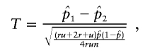where n is the number of sibships, each with r affected sibs, and u is the number of unrelated controls matched to each sibship,

and and are the estimated SNP allele frequency for the ASPs and the controls, respectively. For the design with 250 ASPs and 500 controls, r=2, u=2, and n=250.

Table 5 shows that, for most of the models we considered and especially for recessive models, our test has greater power than the Pearson’s χ²₂ test. Our test is less powerful than Risch and Teng’s test for the additive models examined. This is because Risch and Teng’s test is a 1-df test, whereas our test relies on the estimation of several disease model parameters, resulting in more degrees of freedom. We found that when assuming a prespecified disease model (e.g., additive, dominant, or recessive) by imposing constraints on penetrances estimated in our model, the power of the two tests became comparable (data not shown). This suggests that fixing some disease model parameters is likely to improve the power if these parameters can be approximated from previous studies. Note that neither our test nor Risch and Teng’s test controls for population stratification.

Table 5.

Power (%) Comparison with Other Tests of Association^[Note]

	Dominant		Additive		Recessive
Design, pD=pA, and r2	TLE	χ22	TLE	χ22	TLE	χ22
Case-control:
.1:
.25	12	10	8	9	10	5
.50	26	25	22	25	32	15
.75	43	42	41	44	63	32
1.00	63	62	55	57	86	52
.3:
.25	12	11	14	13	12	7
.50	35	32	28	26	37	22
.75	60	53	50	48	68	44
1.00	79	70	67	65	89	68
	TLE	R & T	TLE	R & T	TLE	R & T
ASP-control:
.1
.25	26	34	31	37	31	19
.50	58	66	62	70	76	43
.75	81	84	83	87	93	60
1.00	93	93	91	93	99	70
.3:
.25	26	29	25	32	26	26
.50	59	61	54	63	65	54
.75	86	83	81	86	91	78
1.00	96	93	91	93	99	86

Note.— Results are based on 2,000 replicate data sets. All models have disease prevalence of K=5% and sibling recurrence risk ratio of λ_s=1.02. R & T = Risch and Teng’s⁵ test. Power is assessed at the 1% level.

Combining Data from Different Family Structures

A key advantage of our method is its ability to combine data from different sampling units. In many association studies, particularly those that follow an initial linkage study, an investigator may have different sampling units available. For example, the data may contain nuclear families with different numbers of genotyped parents and affected and unaffected siblings collected for the initial linkage analysis and unrelated affected or unaffected individuals from additional sampling. A simple strategy for analyzing such data would be to use all unrelated affected individuals and one affected sibling per sibship to form the case group and then use all unrelated unaffected individuals to form a control group. However, this does not use all available data and can give variable results, depending on which affected siblings are selected.⁷

To assess the gain in power by using all available data simultaneously, we simulated different combinations of ASPs, DSPs, unrelated cases, and unrelated controls. We compared the power of our test when using all available data with tests that use only partial data obtained by selecting one sibling per sampling unit. Table 6 suggests that there could be a substantial loss of power when only a subset of the data is used. As expected, when the proportion of data being used decreases, the loss of power increases, suggesting that when the majority of the data are sampled from sibships or families, it is important to use all available data.

Table 6.

Power (%) Comparison with Complete Data and Partial Data

	With All Individuals		With Subset ofUnrelated Individuals
q and Model	No. of Genotypes	TLEa	No. of Genotypes	TLEb
1/2c:
Dominant	600	44	300	31
Recessive	600	80	300	49
Additive	600	22	300	11
2/3d:
Dominant	600	54	400	39
Recessive	600	79	400	54
Additive	600	41	400	21
3/4e:
Dominant	600	54	450	41
Recessive	600	76	450	55
Additive	600	42	450	24

^aPower is estimated using all available data.

^bPower is estimated using one sibling per ASP and unrelated cases as the case group and the unaffected sibling per DSP and unrelated controls as the control group. q is the proportion of individuals used in the analysis for whom there was partial data. Results are based on 2,000 replicate data sets with population disease prevalence of K=5%, sibling recurrence-risk ratio of λ_s=1.02, allele frequency of p_D=p_A=0.3, and r²=1. Power is assessed at the 1% level.

^cSampling units: 150 ASPs and 150 DSPs.

^dSampling units: ASPs, 100 DSPs, 100 cases, and 100 controls.

^eSampling units: 75 ASPs, 75 DSPs, 150 cases, and 150 controls.

As when deciding to genotype all affected siblings or only one sibling per ASP, we found that including the genotypes of all affected family members increases power. When it is not cost-effective to do this additional genotyping for all markers, it could be considered for an additional follow-up phase.

Discussion

We have developed a unified likelihood framework to test for disease-marker association that allows the analysis of sibships of arbitrary size and disease-phenotype configuration. Our likelihood calculations allow us to accommodate different association-study designs and to compare their efficiencies. By use of simulation studies, we found that when the number of individuals to be genotyped at the candidate SNP is fixed, for single-locus models, the one sibling per ASP–control design was generally most powerful, followed by the ASP-control design. As others have noted⁶, we also found that familial cases contributed more association information than did singleton cases and that the DSP design was less powerful than designs that include unrelated unaffected individuals. This pattern holds for disease prevalence 2%⩽K⩽20%, with similar relative efficiency for the seven study designs that we considered (data not shown). Additional simulations reveal that our conclusions regarding the relative efficiency of different study designs remain unchanged at more-stringent critical values (α=.0001, .00001, and .000001).

In most of our simulations, we generated data in which allele frequencies were identical at the disease and SNP loci. To evaluate the robustness of our model to differences in allele frequency between the two loci, we conducted additional simulations over a broad range of allele-frequency differences. We considered combinations of p_D ∈{.1,.3,.5,.7} and p_A ∈{.1,.3,.5,.7} for dominant, additive, and recessive models. Results of these additional simulations suggest that the relative efficiency of different study designs remains unchanged, although all designs have low power when the allele frequencies are very different, since r² is low.

Our results show that the proposed test is usually more powerful than the Pearson’s χ² test for the case-control design. One reason for this advantage is that our test uses an explicit genetic model for the disease, whereas the Pearson’s χ² test is nonparametric in nature. Our results are consistent with those of Thompson et al.,¹⁸ who showed that even simple modeling assumptions, such as assuming Hardy-Weinberg equilibrium in the general population, increase power of genetic-association studies.

Our method does not depend on transmission disequilibrium and can incorporate parental genotypes when available. To evaluate the potential gain in power afforded by collecting parental genotypes, we generated data sets with 500 controls and 500 parent–affected offspring trios for disease models (table 2). We analyzed the data, first taking into account only genotypes for the 500 unrelated cases and controls (average power=39%; α=.01) and then also incorporating parental genotypes (average power=54%, α=.01). We expect that parental data will be less useful on a per-genotype basis but will still provide useful information on allelic association.

Our method assumes that the superlocus formed by combining the disease and SNP loci is in Hardy-Weinberg equilibrium in the general population. In the presence of population stratification, the Hardy-Weinberg equilibrium assumption may be violated and our test may be invalid. An important step for avoiding population stratification is to carefully match cases and controls on the basis of their genetic background. When the degree of stratification is small, it may be possible to adjust our test statistics with genomic control²⁴ or a similar strategy.

We initially assumed that there is a single disease-predisposing variant in the region. As others have noted,⁵ under this assumption, familial cases tend to be enriched for the disease-predisposing allele and thus create a stronger contrast with unaffected individuals. For diseases that are influenced by multiple genes, the advantage of familial cases will depend on the underlying disease models. Our results indicate that, for disease models for which the test locus has equal or stronger effect than the remaining background disease loci, familial cases provide more association information than do randomly selected cases. This remains true unless the effect size of the test locus is much smaller (e.g., λ_s=1.02) than at least one other untested disease locus (e.g., λ_s=1.6). A similar pattern was observed by Howson et al.¹⁰ for additive and crossover two-locus disease models and by Allison et al.²⁵ for extreme sampling in quantitative trait linkage/association studies.

Our findings have important implications for genetic-association studies of many complex diseases, such as depression and schizophrenia, for which loci of large effect have not been identified. For such diseases, designs with familial cases are likely to be a good choice for the initial association studies. One might consider genotyping additional affected family members for those markers that show suggestive evidence of association. Our findings also have implications for disease for which a major gene is known to play a role—such as many auto-immune disorders for which a strong human leukocyte antigen effect has been demonstrated—and age-related macular degeneration, for which two major loci have been identified.^1,26–30 For these diseases, the standard case-control design might be preferred for detecting genes that contribute only a small fraction of the overall disease risk.

Enabled by improvements in genotyping technologies, association studies are beginning to be conducted genomewide.^1,2 We believe our method will be useful for analyzing the results of these studies. Nevertheless, applying our method to hundreds of thousands of markers may present a computational challenge, because it relies on an iterative procedure to maximize the likelihood of the data under alternative models. If computational resources are limited, one option is to first screen all markers with a computationally inexpensive test and then apply our method to markers that show suggestive evidence of association.

In this article, we focused on comparing efficiency of different study designs when the genotyping cost is fixed. Although familial cases provide more association information than do singleton cases in most settings we considered, familial cases (if not already sampled) are typically more difficult to collect and hence may result in higher phenotyping costs. It would be interesting to investigate the relative efficiency of familial cases and singleton cases, taking into account both genotyping and phenotyping costs, with the goal of minimizing total study cost.

In summary, we have developed a unified statistical framework to test for disease-marker association, using sibships of arbitrary size and disease-phenotype configuration. Our method can be readily extended to allow general pedigrees. We compared the efficiency of seven study designs when the number of individuals to be genotyped at the candidate SNP is fixed. Our results suggest that familial cases are more advantageous than are randomly selected cases when the disease follows a single-locus model. This also appears to be true for multilocus disease models, unless the effect size of the test locus is much smaller than that of at least one untested disease locus. On a cost basis, genotyping one sibling per affected sibship and using existing flanking-marker information provides a powerful design for initial association studies. We believe our findings will be helpful for researchers designing and analyzing complex disease–association studies and will increase power and facilitate genotyping resource allocation. We implemented our method in a C++ program, which can be downloaded from the University of Michigan Center for Statistical Genetics Web site.

Appendix : Parameters for Multilocus Disease Models

Assume the disease is influenced by L unlinked diallelic disease loci. For locus l (1⩽l⩽L), let D_l denote the disease-predisposing allele and d_l denote the low-risk allele. Let f_base denote the baseline penetrance for the genotype in which all disease loci are homozygous for the low-risk allele. For an individual with genotype ∈{d_ld_l,D_ld_l,D_lD_l}, let g_l denote the genotype score that counts the number of the D_l alleles. Further, assume that the penetrance is increased over the baseline by w(g_l). The increment of penetrance depends on the marginal disease model at the corresponding locus. For example, for additive, dominant, and recessive models w(g_l) can be defined as shown in table A1. For an individual with genotype scores (g₁,…,g_L), the corresponding multilocus penetrance is

The individual’s disease status can be determined once the genotype is known. Samples of unrelated cases and controls and familial cases can be simulated as usual.

Tables A2–A4 list disease-model parameters for the additive multilocus-disease models described in this article.

Table A1.

Increment of Penetrance

		w(gl)
Genotype at Locus l	gl	Additive	Dominant	Recessive
dldl	0	0	0	0
Dldl	1	0.5Δl	Δl	0
DlDl	2	Δl	Δl	Δl

Table A2.

Disease-Model Parameters for Figure 3^[Note]

	Additive			Dominant			Recessive
λs,test	fbase	Δtest	Δbackground	fbase	Δtest	Δbackground	fbase	Δtest	Δbackground
1.02	.0264	.0471	.0471	.0255	.0258	.0258	.0435	.1307	.1307
1.05	.0237	.0745	.0471	.0226	.0408	.0258	.0427	.2067	.1307
1.10	.0206	.1054	.0471	.0194	.0578	.0258	.0418	.2924	.1307
1.15	.0182	.1291	.0471	.0169	.0707	.0258	.0412	.3581	.1307
1.20	.0162	.1491	.0471	.0148	.0817	.0258	.0406	.4134	.1307
1.25	.0145	.1667	.0471	.0130	.0913	.0258	.0401	.4622	.1307

Note.— Data are a comparison of five-locus disease models for which the effect size of the test locus increases and the effect size of the four remaining disease loci are fixed. The disease prevalence K is fixed at 5%. The predisposing allele frequency at each locus is fixed at 0.1. The locus-specific sibling recurrence risk ratio, λ_s,test, at the test locus is increased from 1.02 to 1.25, and the locus-specific sibling recurrence risk ratio at the four remaining disease loci is fixed at 1.02. Δ_test is the increment of penetrance at the test locus, and Δ_background is the increment of penetrance at each of the four remaining disease loci.

Table A3.

Disease Model Parameters for Figure 4^[Note]

	Additive		Dominant		Recessive
L	fbase	Δ	fbase	Δ	fbase	Δ
2	.0406	.0471	.0402	.0258	.0474	.1307
4	.0301	.0471	.0304	.0258	.0448	.1307
6	.0217	.0471	.0206	.0258	.0422	.1307
8	.0123	.0471	.0107	.0258	.0395	.1307
10	.0029	.0471	.0009	.0258	.0369	.1307

Note.— Data are a comparison of L-locus disease models for which the effect size of each disease locus is fixed and the number of disease loci increases. The disease prevalence K is fixed at 5%. The predisposing allele frequency at each locus is fixed at 0.1. The locus-specific sibling recurrence risk ratio λ_s at all disease loci is fixed at 1.02. Δ is the increment of penetrance at each locus.

Table A4.

Disease Model Parameters for Figure 5^[Note]

	Additive			Dominant			Recessive
λs,large	fbase	Δsmall	Δlarge	fbase	Δsmall	Δlarge	fbase	Δsmall	Δlarge
1.02	.0264	.0471	.0471	.0255	.0258	.0258	.0435	.1307	.1307
1.1	.0206	.0471	.1054	.0194	.0258	.0578	.0418	.1307	.2924
1.2	.0162	.0471	.1491	.0148	.0258	.0817	.0406	.1307	.4134
1.3	.0129	.0471	.1826	.0114	.0258	.1001	.0397	.1307	.5064
1.4	.0101	.0471	.2108	.0084	.0258	.1155	.0389	.1307	.5847
1.5	.0076	.0471	.2357	.0058	.0258	.1292	.0382	.1307	.6537
1.6	.0053	.0471	.2582	.0035	.0258	.1415	.0376	.1307	.7161
1.7	.0033	.0471	.2789	.0013	.0258	.1528	.0370	.1307	.7735

Note.— Data are a comparison of five-locus disease models for which the effect size of the large-effect background disease locus increases and the effect size of the small-effect disease loci, including the test locus, is fixed. The disease prevalence K=5%. The predisposing allele frequency at each locus is fixed at 0.1. The locus-specific sibling recurrence risk ratio, λ_s,large, at the large-effect background locus is increased from 1.02 to 1.7, and the locus-specific sibling recurrence risk ratio at the four remaining loci, including the test locus, is fixed at 1.02. Δ_large is the increment of penetrance at the large-effect background locus, and Δ_small is the increment of penetrance at each of the four remaining loci.

References

- 1.Klein RJ, Zeiss C, Chew EY, Tsai J-Y, Sackler RS, Haynes C, Henning AK, SanGiovanni JP, Mane SM, Mayne ST, Bracken MB, Ferris FL, Ott J, Barnstable C, Hoh J (2005) Complement factor H polymorphism in age-related macular degeneration. Science 308:385–389 10.1126/science.1109557 [DOI] [PMC free article] [PubMed] [Google Scholar]
- 2.Maraganore DM, de Andrade M, Lesnick TG, Strain KJ, Farrer MJ, Rocca WA, Pant PVK, Frazer KA, Cox DR, Ballinger DG (2005) High-resolution whole-genome association study of Parkinson disease. Am J Hum Genet 77:685–693 [DOI] [PMC free article] [PubMed] [Google Scholar]
- 3.International HapMap Consortium (2003) The International HapMap Project. Nature 426:789–796 10.1038/nature02168 [DOI] [PubMed] [Google Scholar]
- 4.——— (2005) A haplotype map of the human genome. Nature 437:1299–1320 10.1038/nature04226 [DOI] [PMC free article] [PubMed] [Google Scholar]
- 5.Risch N, Teng J (1998) The relative power of family-based and case-control designs for linkage disequilibrium studies of complex human diseases. I. DNA pooling. Genome Res 8:1273–1288 [DOI] [PubMed] [Google Scholar]
- 6.Risch N (2000) Searching for genetic determinants in the new millennium. Nature 405:847–856 10.1038/35015718 [DOI] [PubMed] [Google Scholar]
- 7.Fingerlin TE, Boehnke M, Abecasis GR (2004) Increasing the power and efficiency of disease-marker case-control association studies through use of allele-sharing information. Am J Hum Genet 74:432–443 [DOI] [PMC free article] [PubMed] [Google Scholar]
- 8.Li M, Boehnke M, Abecasis GR (2005) Joint modeling of linkage and association: identifying and quantifying SNPs responsible for a linkage signal. Am J Hum Genet 76:934–949 [DOI] [PMC free article] [PubMed] [Google Scholar]
- 9.Risch N (2001) Implications of multilocus inheritance for gene-disease association studies. Theor Popul Biol 60:215–220 10.1006/tpbi.2001.1538 [DOI] [PubMed] [Google Scholar]
- 10.Howson JMM, Barratt BJ, Todd JA, Cordell HJ (2005) Comparison of population- and family-based methods for genetic association analysis in the presence of interacting loci. Genet Epidemiol 29:51–67 10.1002/gepi.20077 [DOI] [PubMed] [Google Scholar]
- 11.Lander ES, Green P (1987) Construction of multilocus genetic linkage maps in humans. Proc Natl Acad Sci USA 84:2363–2367 [DOI] [PMC free article] [PubMed] [Google Scholar]
- 12.Kruglyak L, Daly MJ, Reeve-Daly MP, Lander ES (1996) Parametic and nonparametric linkage analysis: a unified multipoint approach. Am J Hum Genet 58:1347–1363 [PMC free article] [PubMed] [Google Scholar]
- 13.Baum LE (1972) An inequality and associated maximization technique in statistical estimation for probabilistic functions of Markov processes. Inequalities 3:1–8 [Google Scholar]
- 14.Spielman RS, McGinnis RE, Ewens WJ (1993) Transmission test for linkage disequilibrium: the insulin gene region and insulin-dependent diabetes mellitus (IDDM). Am J Hum Genet 52:506–516 [PMC free article] [PubMed] [Google Scholar]
- 15.Cannings C, Thompson EA (1977) Ascertainment in the sequential sampling of pedigrees. Clin Genet 12:208–212 [DOI] [PubMed] [Google Scholar]
- 16.Epstein M P, Lin X, Boehnke M (2002) Ascertainment-adjusted parameter estimates revisited. Am J Hum Genet 70:886–895 [DOI] [PMC free article] [PubMed] [Google Scholar]
- 17.Nelder JA, Mead R (1965) A simplex method for function minimization. Comput J 7:308–313 [Google Scholar]
- 18.Thompson D, Witte JS, Slattery M, Goldgar D (2004) Increased power for case-control studies of single nucleotide polymorphisms through incorporation of family history and genetic constraints. Genet Epidemiol 27:215–224 10.1002/gepi.20018 [DOI] [PubMed] [Google Scholar]
- 19.Wittke-Thompson JK, Pluzhnikov A, Cox NJ (2005) Rational inferences about departures from Hardy-Weinberg equilibrium. Am J Hum Genet 76:967–986 [DOI] [PMC free article] [PubMed] [Google Scholar]
- 20.Self SG, Liang KY (1987) Asymptotic properties of maximum likelihood estimators and likelihood ratio tests under non-standard conditions. J Am Stat Assoc 82:605–610 [Google Scholar]
- 21.Risch N (1987) Assessing the role of HLA-linked and unlinked determinants of disease. Am J Hum Genet 40:1–14 [PMC free article] [PubMed] [Google Scholar]
- 22.Haldane JBS (1919) The combination of linkage values and the calculation of distances between the loci of linked factors. J Genet 8:299–309 [Google Scholar]
- 23.Risch N (1990) Linkage strategies for genetically complex traits. I. Multilocus models. Am J Hum Genet 46:222–228 [PMC free article] [PubMed] [Google Scholar]
- 24.Devlin B, Roeder K (1999) Genomic control for association studies. Biometrics 55:997–1004 10.1111/j.0006-341X.1999.00997.x [DOI] [PubMed] [Google Scholar]
- 25.Allison DB, Heo M, Schork NJ, Wong S-L, Elston RC (1998) Extreme selection strategies in gene mapping studies of oligogenic quantitative traits do not always increase power. Hum Hered 48:97–107 10.1159/000022788 [DOI] [PubMed] [Google Scholar]
- 26.Haines JL, Hauser MA, Schmidt S, Scott WK, Olson LM, Gallins P, Spencer KL, Kwan SY, Noureddine M, Gilbert JR, Schnetz-Boutaud N, Agarwal A, Postel EA, Pericak-Vance MA (2005) Complement factor H variant increases the risk of age-related macular degeneration. Science 308:419–421 10.1126/science.1110359 [DOI] [PubMed] [Google Scholar]
- 27.Edwards AO, Ritter R, Abel KJ, Manning A, Panhuysen C, Farrer LA (2005) Complement factor H polymorphism and age-related macular degeneration. Science 308:421–424 10.1126/science.1110189 [DOI] [PubMed] [Google Scholar]
- 28.Zareparsi S, Branham KE, Li M, Shah S, Klein RJ, Ott J, Hoh J, Abecasis GR, Swaroop A (2005) Strong association of the Y402H variant in complement factor H at 1q32 with susceptibility to age-related macular degeneration. Am J Hum Genet 77:149–153 [DOI] [PMC free article] [PubMed] [Google Scholar]
- 29.Jakobsdottir J, Conley YP, Weeks DE, Mah TS, Ferrell RE, Gorin MB (2005) Susceptibility genes for age-related maculopathy on chromosome 10q26. Am J Hum Genet 77:389–407 [DOI] [PMC free article] [PubMed] [Google Scholar]
- 30.Rivera A, Fisher SA, Fritsche LG, Keilhauer CN, Lichtner P, Meitigner T, Weber BHF (2005) Hypothetical LO C387715 is a second major susceptibility gene for age-related macular degeneration, contributing independently of complement factor H to disease risk. Hum Mol Genet 14:3227–3236 10.1093/hmg/ddi353 [DOI] [PubMed] [Google Scholar]