Coverage and Power in Genomewide Association Studies

Abstract

The ability of genomewide association studies to decipher genetic traits is driven in part by how well the measured single-nucleotide polymorphisms “cover” the unmeasured causal variants. Estimates of coverage based on standard linkage-disequilibrium measures, such as the average maximum squared correlation coefficient (r²), can lead to inaccurate and inflated estimates of the power of genomewide association studies. In contrast, use of the “cumulative r² adjusted power” measure presented here gives more-accurate estimates of power for genomewide association studies.

With millions of validated SNPs now available as a result of the International HapMap Project and other SNP discovery projects, investigators are faced with the decision of which SNPs to use in genomewide association studies. One of the most important factors that investigators must take into account in making this decision is coverage, a measure of how well the genotyped SNPs reflect all variants in the genome. Coverage is determined by the degree of linkage disequilibrium (LD) between SNPs that are in the genotyping set and those that are not. Genomewide association studies will have little power in regions of the genome that are not covered and, in such regions, may fail to find an association when one truly exists.

Several recent articles described large sets of SNPs and their coverage, including an article by Hinds et al.,¹ which described a set of 1.6 million SNPs, and a HapMap study,² which described 1 million SNPs. To measure the ability of their 1.6 million SNPs to cover unobserved SNPs, Hinds et al.¹ compared their SNP set with SNPs from the SeattleSNPs project.³ The SeattleSNPs project has generated an effectively complete set of common (minor-allele frequency [MAF]⩾5%) SNPs in >100 genes by studying 24 European Americans and 24 African Americans. By including the same subjects used in the SeattleSNPs project in the development of their own SNP set, Hinds et al.¹ were able to examine directly the LD between their set and the effectively complete SeattleSNPs set. They also limited the effect of variation in SNP ascertainment due to sample size by examining only SNPs with an allele frequency ⩾10%.

Hinds et al.¹ presented two metrics of coverage (table 1). The first is a threshold metric—that is, the percentage of all known SNPs above a given LD (r²) threshold with measured SNPs:

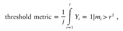where j is the number of all known SNPs and Y_i is an indicator variable that equals 1 if the maximum r² for that SNP, m_i, is greater than a given r² value and equals 0 if it is not.

Table 1.

Average and Threshold Coverage Metrics from Two Studies^[Note]

Study and Sample	SNPs with Maximum r2>.8 (%)	Average Maximum r2
Perlegen:
African American	54	.72
European American	73	.84
HapMap:
Yoruban African	45	.67
CEPH European American	74	.85
Chinese and Japanese	72	.83

Note.— The Perlegen study compared Perlegen SNPs with SeattleSNPs, and the HapMap study compared HapMap SNPs with ENCODE SNPs.

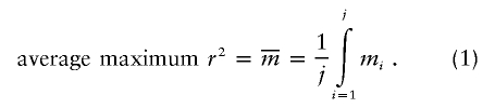
The second metric is the average maximum r², which is the average across all SNPs of the highest r² value between each known SNP and any measured SNP:

For the European Americans studied, 73% of all common (MAF>10%) SNPs had an r²>0.8 with at least one measured common SNP, and the average maximum r² was 0.84. For the African Americans studied, the values were lower, with 54% of all common SNPs having an r²>0.8 with at least one measured common SNP, and the average maximum r² was 0.72. These values demonstrate that the majority of common SNPs in the SeattleSNPs data set are highly correlated with the SNPs selected by Hinds et al.¹

The HapMap study presented a similar analysis—in this case, it was a simulated comparison of 1 million HapMap SNPs with data from the ENCODE study in which 48 subjects were completely resequenced for 10 regions 500 kb in length (table 1). Here, the analysis examined three groups: one with 16 Yoruban African subjects, one with 16 CEPH European American subjects, and one with 8 Chinese and 8 Japanese subjects. By use of the r²>0.8 threshold metric of coverage, the HapMap SNPs provided coverage of 45%, 74%, and 72% for the Yoruban African, European American, and Asian populations, respectively. By use of the average metric of coverage, the average maximum r² for HapMap SNPs for the three populations was 0.67, 0.85, 0.83, respectively.

The LD measure r² is directly related to the sample size required to detect an unmeasured causal variant by use of another measured variant. Specifically, sample size must be increased by a factor of 1/r² to detect an unmeasured variant, compared with the sample size for testing the variant itself.^4,5 The implicit assumption in presenting threshold and average r² metrics of large sets of SNPs is that studies will have sufficient power in using these SNP sets if the sample size is increased by the reciprocal of the threshold value or average maximum r².

The required sample size for a desired level of power is not, however, a simple function of 1/(threshold r²) or 1/(average maximum r²). The power to detect a causal variant is a function of sample size, n; the maximum r² value, m; and all other parameters that affect power (effect size, disease-allele frequency, etc.), which we denote here as y. Thus,

where β is the type II error.

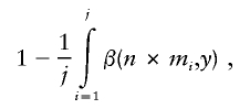
Power can be expressed as a function of the effective sample size, which is the product of the sample size and the maximum r² value. The average maximum r² adjusted power is then

where is as given in equation (1).

Since there is often a widespread distribution in r² values, which are both greater and less than the average or threshold value, the average and threshold r² metrics can give inaccurate estimates of the power of a study. Instead, a metric that correlates more directly with power uses the cumulative distribution of maximum r² values—that is, the “cumulative r² adjusted power,” which equals

where j is the number of potentially causal variants and m_i is the maximum r² for a given SNP. This is equivalent to the weighted sum of the power for sample sizes adjusted for each r² threshold. Thus, the cumulative r² adjusted power equals

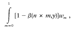where m is the r² threshold; n is the actual, unadjusted sample size; 1-β(n×m,y) is the power for each maximum r² value, determined by the adjusted sample size, n×m; and w_m is the percentage of all SNPs with the particular maximum r² value.

To compare the cumulative r² adjusted power with the power expected using the average maximum r² metric, we used information from the study by Hinds et al.¹ (and from personal communication with D. Hinds) (fig. 1). Tagging SNPs (tSNPs) were chosen using a pairwise r²-based LD bin method (see the article by Hinds et al.¹ for additional details). We used the simple but powerful model of a population-based case-control study and a range of allele frequencies (0.01–0.99) and odds ratios (ORs) (1.2–2.0) under a multiplicative model, with various α levels (0.05 to 10⁻⁸) and a range of sample sizes from 100 cases and 100 controls to 3,000 cases and 3,000 controls. To look at the effect of varying each parameter on study power, we chose the initial parameter values to be allele frequency 0.3, OR 1.5, α level 10⁻⁶, and a sample size of 1,000 cases and 1,000 controls. We then varied each parameter individually, keeping the other parameters constant. All power calculations were performed using the software Quanto^,6 version 0.5.

Figure 1.

Cumulative distribution of maximum r² values from the study by Hinds et al.¹

Results from our comparisons are given in figure 2. The greatest differences in estimates between the average r² adjusted power and cumulative r² adjusted power occurred in the range generally required to detect effects (i.e., power>80%). Looking first at the effect of sample size, we found that estimates for the average maximum r² adjusted power were similar or slightly less than those for the cumulative r² adjusted power when the sample size was <1,600 subjects (800 cases and 800 controls) for the European American sample and <1,800 subjects (900 cases and 900 controls) for the African American sample (i.e., for low values of power in fig. 2A). For larger sample sizes (i.e., when power was >50%), the average metric provided estimates of power that were inflated relative to the cumulative metric. The greatest difference between estimates for the European American group was 12% (98% for average metric vs. 86% for cumulative metric), which occurred at a sample size of 2,800 subjects. For the African American group, the greatest difference was 20% (97% vs. 77%), which occurred at a sample size of 3,200 subjects.

Figure 2.

Effects of varying parameter values on average and cumulative r² adjusted power. Plots are based on a case-control study with 1,000 cases and 1,000 unmatched controls, disease-allele frequency 0.3, OR 1.5, α level 10⁻⁶, and a log additive (multiplicative) model. For each plot, power was calculated by varying one parameter while holding the other parameters constant. AA = African American; EA = European American. A, Sample size is varied from 100 cases and 100 controls to 3,000 cases and 3,000 controls. B, OR is varied from 1.2 to 2.0. C, Disease-allele frequency is varied from 0.01 to 0.99. D, The α level is varied from 10⁻⁸ to 0.05.

In examining a range of ORs, we found that the average metric provided similar or lower estimates of power than those from the cumulative metric for ORs <1.5 (i.e., for low values of power in fig. 2B). For ORs >1.5, the average metric provided inflated estimates of power, with the greatest difference between the two metrics occurring at OR 1.7. Here, the difference between the average and cumulative metrics was 11% (99% vs. 88%) in European Americans and 21% (96% vs. 75%) in African Americans.

Allele frequency also had an effect on the difference between estimates of power from the two metrics (fig. 2C), with the average metric providing inflated estimates at allele frequencies between 0.3 and 0.7. The greatest difference in estimates occurred at an allele frequency of 0.5 for both European Americans (9% difference [89% vs. 80%]) and African Americans (12% difference [76% vs. 64%]).

In addition, the two metrics differed in their estimates of power across the range of α levels examined (fig. 2D). At α⩽10^-7, the average metric provided an underestimate of power, compared with the cumulative metric estimate. At α>10^-7, the average metric provided an inflated estimate of power, with the greatest difference occurring at α=10^-4 for both European Americans (10% difference [98% vs. 88%]) and African Americans (17% difference [93% vs. 76%]).

Both the average and cumulative r² adjustments can be used to determine the sample size increase required to achieve the same power as testing variants directly. Compared with the sample size of a study that has 80% power to test variants directly, given our baseline parameters (described above), sample size must be increased 21% for the European American sample and 46% for the African American sample, if tested using the average maximum r² metric. If the cumulative adjusted r² metric is used, considerably larger sample size increases of 41% for the European American sample and 134% for the African American sample will be required (table 2). In both cases, use of the average maximum r² metric results in an underestimate of the increase in sample size required for sufficient power.

Table 2.

Sample Size Increases Required for 80% Power with Average and Cumulative r² Adjustments

	Sample Size Increase (%)for 80% Powera with
Sample and SNPs	Average r2 Adjustment	Cumulative r2 Adjustment
European American:
All SNPs	21	41
tSNPs	27	48
African American:
All SNPs	46	134
tSNPs	50	139

^aPower for a case-control study with one unmatched case per control, disease-allele frequency 0.3, OR 1.5, α level 10⁻⁶, and a log additive (multiplicative) model.

The differences in estimated power and required sample sizes between these coverage metrics are mainly because of the percentage of SNPs that are in low LD with the SNPs in the genotyping set. An example of this can be seen in figure 2A, in which large increases in sample size provide nearly complete power for the average metric but not for the cumulative metric. The difference is more pronounced in the African American sample, which has a higher density of SNPs with low values of maximum r² than does the European American sample. This also drives the differences in estimated power between the European American and African American groups in terms of the percentage of SNPs having a maximum r²<0.5 with a genotyped SNP (14% and 29%, respectively).

To illustrate this point, we examined the increase in power for various levels of r² when the sample size is increased by 25% and 100% (table 3). Increasing the sample size by 25% led to increases in power of slightly greater than 0.2 for variants with maximum r² values in the range of 0.6–0.8. When the sample size was increased by 100%, the largest increases in power occurred for variants with maximum r² values in the range of 0.4–0.7. In either case, the increase in power for variants with maximum r²<0.3 was considerably less than for variants with maximum r²⩾0.3.

Table 3.

Effects of Sample Size Increases on Power for Various Values of r²

		Powera for Sample Size Increase of
r2	Powera for Initial Sample	25%	100%
.1	.00	.00	.01
.2	.01	.02	.11
.3	.04	.09	.33
.4	.11	.21	.60
.5	.20	.37	.80
.6	.33	.55	.92
.7	.47	.70	.97
.8	.60	.81	.99
.9	.72	.89	1.00
1	.80	.94	1.00

^aPower for a case-control study with one unmatched case per control, disease-allele frequency 0.3, OR 1.5, α level 10⁻⁶, and a log additive (multiplicative) model.

In addition to the use of the cumulative distribution, a gold standard measure of coverage for a large SNP set must be determined by comparing that set with one or more SNP sets that are ascertained by full resequencing of genomic regions, such as the SeattleSNPs³ and ENCODE⁷ SNPs. Although both of these projects examined 48 subjects, they used different sampling methods, which could lead to different estimates of coverage. SNP sets that are used to test coverage must examine a sufficient number of chromosomes to fully ascertain SNPs of a given frequency.⁸ Examining coverage within a SNP set rather than against a comprehensive register of SNPs can overstate coverage because of the structure of LD—in particular, the presence of LD holes—in the human genome.^9,10

Finally, any gold standard measure of coverage should also be determined using a population similar to the one used in the genomewide association study. The frequency of copy-number polymorphisms can vary by population,¹¹ as can undetected variation in primer sequences, leading to unforeseen genotyping errors and a further reduction in power. In addition, variation in LD patterns between populations can lead to inaccurate assumptions about coverage. For example, with the use of the Hinds et al.¹ SNP set, a study with a sample size large enough to provide an adjusted power of 80% for the European American sample would provide an adjusted power of only 65% for the African American sample (fig. 2). Ignoring the appropriate metric can lead to overestimates of power and a larger number of false-negative results than expected.

References

- 1.Hinds DA, Stuve LL, Nilsen GB, Halperin E, Eskin E, Ballinger DG, Frazer KA, Cox DR (2005) Whole-genome patterns of common DNA variation in three human populations. Science 307:1072–1079 10.1126/science.1105436 [DOI] [PubMed] [Google Scholar]
- 2.Altshuler D, Brooks LD, Chakravarti A, Collins FS, Daly MJ, Donnelly P (2005) A haplotype map of the human genome. Nature 437:1299–1320 10.1038/nature04226 [DOI] [PMC free article] [PubMed] [Google Scholar]
- 3.Crawford DC, Carlson CS, Rieder MJ, Carrington DP, Yi Q, Smith JD, Eberle MA, Kruglyak L, Nickerson DA (2004) Haplotype diversity across 100 candidate genes for inflammation, lipid metabolism, and blood pressure regulation in two populations. Am J Hum Genet 74:610–622 [DOI] [PMC free article] [PubMed] [Google Scholar]
- 4.Risch N, Teng J (1998) The relative power of family-based and case-control designs for linkage disequilibrium studies of complex human diseases I. DNA pooling. Genome Res 8:1273–1288 [DOI] [PubMed] [Google Scholar]
- 5.Pritchard JK, Przeworski M (2001) Linkage disequilibrium in humans: models and data. Am J Hum Genet 69:1–14 [DOI] [PMC free article] [PubMed] [Google Scholar]
- 6.Gauderman WJ (2002) Sample size requirements for association studies of gene-gene interaction. Am J Epidemiol 155:478–484 10.1093/aje/155.5.478 [DOI] [PubMed] [Google Scholar]
- 7.ENCODE (2004) The ENCODE (ENCyclopedia Of DNA Elements) Project. Science 306:636–640 10.1126/science.1105136 [DOI] [PubMed] [Google Scholar]
- 8.Kruglyak L, Nickerson DA (2001) Variation is the spice of life. Nat Genet 27:234–236 10.1038/85776 [DOI] [PubMed] [Google Scholar]
- 9.Wall JD, Pritchard JK (2003) Assessing the performance of the haplotype block model of linkage disequilibrium. Am J Hum Genet 73:502–515 [DOI] [PMC free article] [PubMed] [Google Scholar]
- 10.Ke X, Hunt S, Tapper W, Lawrence R, Stavrides G, Ghori J, Whittaker P, Collins A, Morris AP, Bentley D, Cardon LR, Deloukas P (2004) The impact of SNP density on fine-scale patterns of linkage disequilibrium. Hum Mol Genet 13:577–588 10.1093/hmg/ddh060 [DOI] [PubMed] [Google Scholar]
- 11.Jorgenson E, Tang H, Gadde M, Province M, Leppert M, Kardia S, Schork N, Cooper R, Rao DC, Boerwinkle E, Risch N (2005) Ethnicity and human genetic linkage maps. Am J Hum Genet 76:276–290 [DOI] [PMC free article] [PubMed] [Google Scholar]