Multilocus Association Mapping Using Variable-Length Markov Chains

Abstract

I propose a new method for association-based gene mapping that makes powerful use of multilocus data, is computationally efficient, and is straightforward to apply over large genomic regions. The approach is based on the fitting of variable-length Markov chain models, which automatically adapt to the degree of linkage disequilibrium (LD) between markers to create a parsimonious model for the LD structure. Edges of the fitted graph are tested for association with trait status. This approach can be thought of as haplotype testing with sophisticated windowing that accounts for extent of LD to reduce degrees of freedom and number of tests while maximizing information. I present analyses of two published data sets that show that this approach can have better power than single-marker tests or sliding-window haplotypic tests.

Although results that are based on simulated and real data have been mixed, it is generally appreciated that multilocus methods have higher potential for powerful detection of trait-marker associations than do single-marker methods.^1–3 However, this potential has not yet been fully realized because of difficulties balancing degrees of freedom or number of tests with maximal extraction of information.

I propose a new approach that is based on inhomogeneous variable-length Markov chains (VLMCs). These are higher-order Markov chain models in which the length of memory of the process depends on the context. Thus, in regions of high linkage disequilibrium (LD) between markers, the models will have a longer memory, whereas, in regions of low LD, the memory will be short. I fit these graph models using haplotype data from all individuals and then test for association between trait data and graph-edge counts. The focus in this study is on case-control traits, but I consider quantitative traits in the “Discussion” section.

My proposed method has several advantages. It is easy to apply, with no need to choose a haplotype-window size or to select tagging markers. The method automatically balances degrees of freedom and number of tests with maximal information extraction, which results in high power to detect association. The results are simple to interpret and robust to low haplotype frequencies. There is flexibility to choose different types of association tests and to adjust for covariates. The method has the potential for efficient implementation and application to whole-genome scan data (hundreds of thousands of markers).

In the remainder of this section, I give a brief review of existing multilocus methods, with focus on unresolved issues that the proposed method can help to resolve. The “Methods” section describes the VLMC model framework, gives an algorithm for fitting the model to genetic data, and outlines the testing procedure. In the “Results” section, I present results from analysis of two published data sets, demonstrating the power of my method. In the “Discussion” section, I provide ideas for extension of the method to unphased data and for the analysis of quantitative traits and adjustment for covariates.

The standard approach to multilocus case-control analysis is haplotype analysis, typically with use of an expectation-maximization (EM) algorithm to account for uncertain haplotype phase. Haplotype frequencies can be inferred⁴ and then used in various types of association tests, or a likelihood ratio test can be used that incorporates the EM algorithm.⁵ Some related approaches, such as multilocus scoring,⁶ do not make use of phase information and are thus computationally more efficient. To have a test that is robust (i.e., gives correct type I error rates, even in the presence of low haplotype frequencies), it is common to apply permutation testing, in which the trait values are permuted and the test statistic is recalculated a large number (usually thousands) of times. Alternative approaches for ensuring robustness of the test include dropping or combining haplotype categories with low counts, which also reduces degrees of freedom of the test, or the use of Fisher’s exact test, provided the number of haplotype categories is small enough for this to be computationally feasible.

In assessing a small number of markers in a region of high LD, it is sensible to include all markers in a single haplotype test. Complexities arise when a large candidate gene, an extended region under a linkage peak, or a whole chromosome from a genome-association scan is considered. LD typically follows a complex pattern, so it is unclear which markers should be considered jointly in a haplotype analysis. Although a block structure is often seen in haplotype data, the blocks do not capture the full picture, with some haplotypes extending over several blocks,⁷ and definitions of haplotype blocks can be somewhat arbitrary.

A sliding-window approach is commonly used to apply haplotype analysis over a large region. One chooses a window size (generally small, for computational reasons) and slides it along the region of interest, calculating a test statistic in each window.⁸ For example, if a window of size 5 is chosen, markers 1–5 will make up the first haplotype test, markers 2–6 the second, and so on. This approach does not adapt to the degree of LD, which can vary greatly throughout a region. If the window size is too small for the degree of LD, information is lost, whereas, if the window size is too large, excessive noise is introduced. An exhaustive approach can be taken, in which all window sizes (up to some maximum) are considered,⁹ with adjustment for multiple testing by permutation. Although this brute-force approach has potential, it is currently unfeasible except for small maximum-window sizes. A Markov chain–Monte Carlo algorithm (MCMC) can be used to adapt window sizes on the basis of extent of LD for haplotype-phase estimation,¹⁰ and perhaps such an approach could be adapted for association testing, but it would be computationally intensive.

Cladistic¹¹ and haplotype-similarity¹² methods test for clustering of similar haplotypes within the samples of cases and controls. More-complex developments of these ideas include decay of haplotype sharing,¹³ which uses a hidden Markov model (HMM) for haplotype ancestry to develop a likelihood-based approach to haplotype sharing, and a coalescent-based cladistic approach,¹⁴ which uses MCMC to sample from the space of possible realizations of the coalescent. On large genomic regions, these methods still face the issue of determining which markers to consider simultaneously. For example, a sliding-window approach has been used with cladistic analysis.¹⁵

Several other, more-complex methods for multilocus association analysis exist. In general, these approaches are computationally intensive and often require substantial user input and sophisticated interpretation. They may be most useful as a follow-up for significant results found using simpler methods.

A graphical models approach^16,17 fits graphical Markov models jointly to the marker and trait variables. A parsimonious model is found, and dependencies between the trait and markers are of interest. This type of approach can be extended to genomewide studies by using windows to break the genome into small regions on the basis of LD.¹⁸ Graphical Markov models are similar to VLMCs, in that they involve Markov properties (conditional independence) between variables. Graphical Markov models have less intrinsic reliance on variable (marker) order than do VLMCs, but they cannot allow the memory (i.e., choice of variables on which a conditional probability is based) to depend on the state of some of those variables. Moreover, fitting these models by maximum likelihood is computationally expensive.

Also close in spirit to my proposed method are methods based on HMMs. A first-order Markov chain can be applied to dependencies between haplotype blocks, with MCMC used to find optimal block divisions.¹⁹ Alternatively, one can model the ancestral haplotype state—that is, whether a region on a haplotype is descended from the founder chromosome on which the disease mutation first arose—as a first-order Markov chain along the chromosome.²⁰

VLMCs have some important advantages over HMMs.²¹ With an HMM approach, it is necessary to prespecify the structure of the model, which often involves making many simplifying assumptions about processes of which little is known (e.g., the Markov structure for the ancestral haplotype state²⁰). Also, to fit the HMM model, it is generally necessary to use an iterative approach such as MCMC, which is computationally expensive and requires careful supervision to ensure convergence. In contrast, VLMCs do not require explicit modeling yet are flexible enough to closely approximate HMMs and can be fitted using heuristic methods that are fast and automatic.

VLMCs are not unknown to the statistical genetics field, since they been used in haplotype-phase reconstruction.²² With the use of VLMCs, my proposed method avoids the problem of choosing an appropriate window size, clusters haplotypes to improve power, and employs a computationally efficient heuristic algorithm that does not require sophisticated user input.

Methods

In VLMC models, the “memory” of a Markov chain is allowed to depend on the history of the chain.^21,23 For example, consider a two-state variable–memory-length model with the following properties:

where

This chain has a memory of length 1 if the most recent state (X_t-1) takes the value 1, whereas it has a memory of length 2 if the most recent state takes the value 2. In my application, the variable X_t represents the allele at marker t.

A model for alleles at markers along a chromosome must necessarily be inhomogeneous, because transition probabilities and memory length vary from one position to another. An inhomogeneous VLMC can be represented by a directed acyclic graph. Figure 1 shows an example of the graph of a model of a region composed of haplotype blocks. Note that the proposed method does not require the existence (or prespecification) of a haplotype-block LD structure. (In figs. 2–7, the directionality of the graph is not shown, but it is implied [from left to right].) See also figures 3 and 5, which show models fit to real data.

Figure 1.

VLMC model for a region containing three haplotype blocks. Solid arrows represent SNP allele 1; dashed arrows represent SNP allele 2. Edges to be tested are marked “T.”

Figure 2.

A, Tree graph constructed using the haplotype data in table 1. Circles represent nodes, and the values in them represent level and node identifier within level; for example, “3.2” denotes node 2 at level 3. A solid edge between nodes at levels i and i+1 represents allele 1 at SNP marker i; a dashed edge represents allele 2. Numbers above edges represent haplotype counts. Thus, 137 over the edge between 3.3 and 4.4 represents 137 haplotypes that have allele 2 at the first SNP, 1 at the second SNP, and 1 at the third SNP. Although directional arrows are not shown, a left-to-right direction is implied. B, The graph from figure 2A after merging. Nodes 3.1 and 3.3 in figure 2A have been merged, as have all nodes at level 5. Notation is as described for panel A. Edges to be tested are marked with “T.”

Figure 3.

Model fitted to the cystic fibrosis region-coded data. Each of the various line patterns represents an allele code (alleles A–H²⁵). The nodes are shown as circles, with area proportional to the total count for the node.

Figure 4.

P values for tests of association between the region markers and cystic fibrosis: Fisher’s exact single-marker allelic test P values (○); graph-edge test P values (×).

Figure 5.

Model fitted to the cystic fibrosis RFLP data. Solid lines represent allele 1; dashed lines represent allele 2. The nodes are shown as circles, with area proportional to the total count for the node.

Figure 6.

P values for tests of association between the RFLP markers and cystic fibrosis: Fisher’s exact single marker allelic test P values (○); graph-edge test P values (×).

Figure 7.

P values for tests of association between the genetic markers and Crohn disease: Fisher’s exact single marker test P values (○); graph-edge test P values from the model fit to markers 1–60 (+) and from the model fit to markers 44–103 (×).

A VLMC model captures the LD structure in the genetic data and allows us to test for associations with a trait in an automated yet sensible way. Each edge of the graph represents a cluster of haplotypes that are tested for association with the trait (further described below).

Ron et al.²⁴ presented an algorithm for fitting inhomogeneous VLMCs. Their algorithm is applied to cursive writing and spoken words, and only one letter or word is modeled at a time. I give a brief description of the algorithm, along with details of modifications I made to enable the algorithm to handle much longer sequences of information and to focus on obtaining a parsimonious model. The reader is referred to Ron et al.²⁴ for more-detailed information.

To describe my algorithm, I will first make some comments and provide notation. The directed acyclic graph representing the VLMC model has the property of being leveled.²⁴ Each node of the graph has a level that corresponds to a position in the sequence of markers. At level 1, there is only one node, which does not itself contain information. A node at level d (d=2,3,…,D+1, where D is the number of markers) represents a history or collection of possible allele sequences (i.e., haplotypes) up to and including marker d-1. Each edge originating from a node at level d (d=1,2,…,D) terminates at a node in level d+1. An edge marked by allele a and originating from node x at level d represents the event of allele a at marker d following the history represented by node x and thus also represents a collection of haplotypes involving alleles at markers up to and including marker d.

When two edges are directed into the same node, the history of this node represents a union of the two histories represented by the incoming edges. This feature represents historical recombination. In terms of the probabilistic model, this represents a Markov (loss of memory) property. For example, consider node 3.1 in figure 2B. This node represents the collection x={x₁,x₂} where x₁ represents the haplotype 2,1 (allele 2 at the first marker and allele 1 at the second), whereas x₂ represents the haplotype 1,1. Let A be the random variable representing the sequence of alleles at markers 3 and 4. Given the graph, P(A|x₁)=P(A|x₂)=P(A|x); that is, the conditional probability of A given x does not depend on whether the alleles at the previous two markers were given by x₁ or x₂.

My algorithm starts by taking phased haplotype data (without regard to trait status) and putting it into a tree graph. Each path from the root to a terminal node of the tree represents a distinct observed haplotype. Figure 2A shows an example that corresponds to the data in table 1 (which consists of 300 case and 300 control haplotypes on four biallelic markers). Starting from the root of the tree (level 1) and working down the levels, the algorithm checks to see if nodes at the same level can be merged. Merging of nodes corresponds to recognizing decay of memory in the model. Two nodes are merged if the transition probabilities corresponding to all downstream (descendant) nodes are sufficiently similar. In the appendix, I give my criterion for determining which nodes to merge, which is similar to that of Ron et al.²⁴ Figure 2B shows the graph from figure 2A after merging has occurred. Note that the decision to merge nodes 3.1 and 3.3 in this graph also results in the downstream merging of nodes 4.1 and 4.4 and of nodes 4.2 and 4.5.

Table 1.

Haplotype Counts for Figure 2A

	Count
Haplotype	Total	Case	Control
1111	21	12	9
1112	79	43	36
1122	95	43	52
1221	116	59	57
2111	25	14	11
2112	112	60	52
2122	152	69	83

Merging proceeds at each level in turn, and all nodes at the final level are always merged. Once the model has been fitted to the combined (case and control) data, one can go through the model to determine specific case and control counts (or distribution of other trait variables) that correspond to each edge. Given any haplotype sequence, one can follow its path through the graph by following the sequence of alleles. For example, in the graph in figure 2B, haplotype 2112 corresponds to the path from node 1.1 through nodes 2.2, 3.1, and 4.1 to node 5.1 (via the dashed edge between nodes 4.1 and 5.1).

At each edge of the graph, one can test for association with trait status. For example, consider the edge from node 3.1 to node 4.1 (fig. 2B) with the data in table 1. This edge corresponds to haplotypes of the form *11*, where the asterisk (*) represents an arbitrary allele, with 129 case haplotypes and 108 control haplotypes in total, compared with 171 case and 192 control haplotypes not on this edge, which results in a P value of .095 with Fisher’s exact test.

Not every edge of the graph needs to be tested, since many edges represent the same or similar haplotype clusters, whereas other edges have counts that are too low to be worth testing. Haplotype clusters change at points of splitting or merging in the graph. For example, the split at node 2.1 of figure 2B divides the haplotype cluster consisting of haplotypes of the form 1*** into a cluster containing haplotypes of the form 11** and a cluster containing haplotypes of the form 12**. The merge at node 3.1 of figure 2B combines a cluster containing haplotypes of the form 11** with a cluster containing haplotypes of the form 21**. Call an edge a “splitting edge” if it is one of two or more edges directed out of a node, whereas an edge is called a “merging edge” if it is one of two or more edges directed into a node. An edge that is not splitting or merging represents exactly the same haplotype cluster as one or more other edges; for example, the edge from node 3.2 to node 4.3 in figure 2B represents the same cluster (haplotype 1221) as does the edge from node 2.1 to node 3.2 or the edge from node 4.3 to node 5.1. A splitting edge that is not also a merging edge represents either the same haplotype cluster as some merging edge farther on in the graph, or, if further splitting occurs before merging, represents a supercluster that combines two or more haplotype clusters represented by merging edges farther on in the graph. Such superclusters tend to reflect the sequential nature of the VLMC model rather than inherent biological phenomena. On the other hand, merging reflects historical recombination. Thus, merging edges tend to more fully reflect the haplotype clusters of biological interest than do splitting edges.

I test only merging edges (edges that merge with others into a node). Edges with very low counts are ignored in this merging criterion, so that if an edge with a large count merges with an edge with a count of just 1 or 2 and does not merge with any other edges, I do not test either of these edges. In figure 1, I would test the haplotype clusters corresponding to the edges marked with “T” (assuming all edge counts are sufficiently high). In this way, I test all haplotype clusters found in the graph, except that superclusters that split before merging will not themselves be tested, although their component subclusters are tested. For example, in block 2 of figure 1, haplotypes 112 and 121 are tested individually, but the edge containing both haplotypes together is not tested. In figure 1, the tests include all haplotypes within each haplotype block. In addition, haplotype clusters *211 (where the asterisk [*] denotes an arbitrary allele) and **11 in block 1 are tested. These clusters indicate that the algorithm is responding to apparent historical recombination between markers 1 and 2 and between markers 2 and 3 within this block. Also, in the results presented here, I do not test an edge if the total count for the edge is <50. (In general, the threshold chosen should depend on the strength of signal expected—for a low frequency haplotype with high penetrance, a small threshold should be used, whereas a higher threshold is appropriate for common haplotypes with low penetrance.) Figure 2B shows the edges to be tested in that graph. Note that the solid edge from node 4.1 to node 5.1 is not tested, even though it is a merging edge, because it has a count of <50.

Fisher’s exact test is particularly appropriate for testing, since it is exact rather than asymptotic and can deal with the small counts that often occur in haplotype data. However, provided that the edges with low counts are not tested, Pearson’s χ² test is also appropriate. In the results presented here, I use Fisher’s exact test because I wish to accurately compare very small P values.

For comparison with results from my method, I present results from single-marker and haplotypic tests. The single-marker tests are allelic tests performed using Fisher’s exact test, with one test per marker. The haplotypic tests use the same estimated haplotypes that go into my model. I chose not to use EM-based haplotypic tests that would sum over possible haplotypes, since the haplotype phases are fairly well determined by family data in the two data sets considered. As with tests using my model, I test individual haplotypes and do not consider a haplotype if the total count (cases and controls) for the haplotype is <50, to reduce the number of tests considered. I note that, for these data, the same smallest P values are found when testing all haplotypes or graph edges (including those with count <50), even though many more tests are required.

To investigate the type I error of my method and to obtain thresholds for experimentwise significance, I permuted case-control status to simulate data under the null hypothesis of no marker-trait association. For each permutation, P values were calculated using the new case-control values. Note that the graph itself stays the same in each permutation, since it is not dependent on case-control status. Similarly, the same set of edges satisfies the criteria for testing in each permutation.

Software

I have implemented the algorithm in R, and my code is freely available from the HapVLMC Web site. This prototype implementation has suboptimal memory handling so can only process ∼60 markers at a time; however, we are developing an improved version that should be able to handle an unlimited number of markers. Note that the computational time for the merging algorithm is approximately linear in relation to the number of markers, so that, for large numbers of markers, the most important programming consideration is efficient use of memory.

Cystic Fibrosis Data

I considered data consisting of 94 cystic fibrosis (MIM 219700) haplotypes and 92 control haplotypes.²⁵ I used PHASE v2.1.1^26,27 to estimate missing data and unresolved phase. I analyzed the data two ways, one using the nine haplotype regions (each region gives a multiallelic marker with up to eight alleles) defined by Kerem et al.,²⁵ and the other using the 23 biallelic RFLP markers directly.

Crohn Disease Data

I considered data consisting of 258 individuals with Crohn disease (MIM 266600) and their parents, genotyped on 103 SNPs in a 500-kb region on chromosome 5q31.²⁸ I used Merlin²⁹ to determine haplotype phase for the trios, followed by PHASE v2.1.1 to estimate missing genotypes and unresolved phase. I split the parental haplotypes into 258 haplotypes transmitted to the affected offspring (the “case” haplotypes) and 258 untransmitted haplotypes (the “controls”). The 5q31 region has extensive LD, so it has proven difficult to localize the causative mutations for Crohn disease in this region.³⁰

Results

Cystic Fibrosis Data

The cystic fibrosis data have a very strong signal, so test P values tend to be extremely small. Figure 3 shows the graph fitted to the nine multiallelic regional markers. The results of the graph-edge tests are shown in figure 4, with results of single-marker allelic tests for comparison. Some levels have more than one P value, because more than one edge was tested. Other levels have no graph-edge P values, since no edges at those levels satisfied the testing criteria, either because the edges had insufficient counts or because LD is sufficiently strong that the corresponding clusters of haplotypes are tested elsewhere.

The smallest graph-edge test P value was 1.9×10^-23 (from nine tests), whereas the smallest single-marker test P value was 3.5×10^-16. For comparison, I ran sliding-window haplotype tests of all window sizes from 2 to 9, testing each haplotype individually with Fisher’s exact test. The smallest of these P values was 1.9×10^-23 (from a total of 26 tests, excluding tests of haplotypes with count <50).

Figure 5 shows the graph fitted to the 23 biallelic RFLP markers. The results of the graph-edge tests (and single-marker allelic tests for comparison) are shown in figure 6. The smallest graph-edge test P value was 3.9×10^-22 (from 14 tests), whereas the smallest single-marker test P value was 6.3×10^-15. For comparison, I again ran sliding-window haplotype tests of all possible window sizes. The smallest of these P values was 1.9×10^-23 (from a total of 199 tests, excluding tests of haplotypes with count <50). In 10,000 permutations of case-control status, I found that the 5th percentile of minimum graph-edge test P values was .008, which is much greater than 3.9×10^-22, so the graph-edge test result is clearly significant after correcting for multiple testing. Also, the proportion of P values that fall below .05 was 0.041, so that the test is shown not to be anticonservative. In fact, since Fisher’s exact test was used, it is redundant to check false-positive error rates, since Fisher’s exact test is always exact or slightly conservative.

To investigate the haplotypes underlying a significant result, one can look at which haplotypes pass through the corresponding edge of the graph. Table 2 shows the haplotypes passing through the most significant edge of the graph that is based on the RFLP markers (the edge corresponding to allele 2 and originating at node 2 of level 19 in figure 5; this is the dashed edge coming out of the second-to-lowest node at level 19 and connecting to the highest node at level 20). One can look at any window of markers, but I chose here to look at markers 7–22, since adding further markers to either end of this window merely increases the number of unique haplotypes observed without adding recognizable pattern. Markers 11–20 exhibit a common haplotype, 2212121121 (shown in bold italics in table 2), shared by all but three haplotypes passing through this edge. It is this haplotype that is driving the results in both the RFLP and region-coding analyses. The ΔF₅₀₈ deletion, which appears to be the cause of 70% of cystic fibrosis cases, is located between RFLP markers 17 and 18 and is found almost exclusively in this particular haplotype background.²⁵

Table 2.

Haplotypes and Frequencies for Markers 7–22 for Most-Significant Edge of Cystic Fibrosis RFLP Graph^[Note]

Haplotype	Frequency
2111221212112111	25
2111221212112122	22
2111221212112121	1
1111221212112122	10
1111221212112111	7
1111221212112121	4
1211221212112111	1
1211221212112121	1
1211221212112122	2
1222221212112122	1
2122112111222122	1
1222112111222122	1
1222112111222111	1

Note.— Markers 11–20 exhibit a common haplotype, 2212121121 (shown in bold italics).

It is unwise to make too much of comparisons of P values that are this small; however, these results demonstrate that my method is competitive with standard single-marker and haplotypic tests on these data. My method does not require the specification of a haplotype-window size yet involves only a fairly small number of tests.

Crohn Disease Data

The prototype software implementation of my algorithm could not handle all 103 SNP markers at once, so I split the data into two overlapping sets: SNPs 1–60 and SNPs 44–103. Figure 7 shows the graph-edge test P values and single-marker allelic test P values.

The smallest single-marker test P value was 3.8×10^-6 at marker 28. This is similar to results obtained with a TDT test (smallest P value 7×10^-6, also at marker 28).³¹ The smallest graph-edge test P value was 2.0×10^-6 (from 81+61 tests). In 1,000 permutations of case-control status, I found that the 5th percentile of minimum graph-edge test P values was .001, which is much higher than 2.0×10^-6, so the graph-edge test result is clearly significant after correcting for multiple testing. For comparison, I ran sliding-window haplotype tests of all window sizes, of which the smallest P value was 5.0×10^-7 (from 8,543 tests, excluding tests of haplotypes with count <50). Although one haplotypic test found a stronger signal than did my method, a huge number of haplotypes were tested to obtain that result.

Rioux et al.³¹ found a single extended-risk haplotype, which is the red (top) haplotype in figure 2a of Daly et al.²⁸ Daly et al.²⁸ provide haplotype-block information for the SNPs in this study. There is extensive LD throughout the region, with the strongest LD stretching from block 4 (starting at SNP 25) through block 9 (ending at SNP 91). It is noteworthy that my most significant result is found on an edge at level 48 of the graph based on SNPs 44–103 and thus represents SNP 91, or the end of this region of strongest LD. My tests are restricted to edges that merge; since merging represents historical recombination, my tests will tend to occur at the end of haplotype blocks, with the tested edges corresponding to clusters of haplotypes within those blocks. I examined the haplotypes passing through the most significant edge, considering markers 44–91 but excluding markers 74, 77, and 85, which fall between blocks or for which either allele may be present in the risk haplotype discussed by Rioux et al.³¹ Of 134 haplotypes on this edge, 98 were identical with the risk haplotype of Rioux et al.³¹ on these markers, whereas only 3 haplotypes on this edge differed in more than four markers from the risk haplotype. In contrast, for haplotypes not on this edge, only 6 (of 382) differed from the risk haplotype in four or fewer markers. Thus, this graph-edge test is detecting the signal found by Rioux et al.³¹ but without requiring definition of haplotype-block structure or extensive haplotype testing.

To investigate the impact of SNP selection on my method, I used the method of Carlson et al.,³² with a threshold of r²>0.8, to select 54 tagging SNPs (tSNPs). The graph fit to the tSNP data is similar to those fit to the unselected data, with up to 15 nodes per level (the graphs fit to the unselected data on SNPs 1–60 and on SNPs 44–103 have up to 17 and 18 nodes per level, respectively). The smallest graph-edge test P value is 1.2×10^-6 (from 69 tests). From these results, it seems that, although the selection of tSNPs is not necessary for the success of my method, it is not detrimental either.

Discussion

I have presented a method for multilocus analysis of haplotype data and have demonstrated, through application to two published data sets, that it is competitive with standard haplotype tests. A major advantage of my method is that it is adaptive to LD, so that there is no need to specify haplotype blocks or a window size for haplotype tests.

My method is computationally feasible for large data sets. The most computationally demanding part is fitting a graph model with the merging process; however, the algorithm is approximately linear in the number of markers and approximately quadratic in the number of nodes per level. The number of nodes per level is bounded by the number of haplotypes, so, with appropriate implementation (which my collaborator and I are developing), it should scale to hundreds of thousands of markers and thousands of individuals. Once the fitting is complete, a variety of tests can be performed, with minor computational effort.

Each P value produced by the method is exact if Fisher’s exact test is used and is at least robust to low haplotype frequencies if Pearson’s χ² test is used with appropriate thresholding. If a single P value is desired to summarize evidence for association over a region or to obtain a threshold for experimentwise significance, permutation testing can be used. At each iteration of the permutation procedure, trait status would be permuted among individuals. Fortunately, since the graph is fitted without regard to trait status, the only part of the procedure that would need to be repeated at each iteration is the testing of each eligible edge, which is computationally fast.

The method is very flexible in terms of data type. It is suitable for multiallelic markers (such as microsatellites) as well as biallelic markers (such as SNPs), as demonstrated through analysis of the cystic fibrosis data. A reasonably large number of individuals is required to obtain a graph that models the underlying LD structures fully; however, the model can be fit with small numbers of individuals and the tests will still be valid, although not as powerful. With just 100 individuals (200 haplotypes) in the cystic fibrosis data, the method performed well.

Phased data with imputed missing values are required as input; however, this is becoming less of an issue. Good haplotype-phasing programs are now available, with improved programs being developed³³ to handle thousands of markers. Moreover, it may not be long before molecular haplotyping is cost-effective.³⁴ An alternative to use of a single estimated haplotype pair for each individual is to take into account all possible haplotype pairs consistent with each individual’s genotype, weighted by the probability of the haplotype pair given the genotype. To do so, haplotype counts are replaced by haplotype weights, and permutation must be used to obtain valid P values.³⁵ Another option is to fit a model by using genotypic data rather than haplotypes and by treating each genotype as an allele. This results in a genotypic-based test that may be more suitable for some disease models than the allelic-based tests I have used here. On the other hand, use of genotypes effectively halves the sample size (each individual has two haplotypes but one multilocus genotype) and results in a less parsimonious graph.

A feature of the fitted graph models is that they start with a single node and build up over the first few levels to a number of nodes per level that reflects the underlying number of ancestral haplotypes in the region. In the final levels of the graph, the number of nodes again decreases because of lack of information to distinguish differences between nodes. These features reflect the reduced amounts of haplotypic information available at the ends of the genotyped region. Thus, in selecting markers to genotype in a region of interest, it is a good idea to extend the genotyping a little beyond the ends of the region on each side.

The core of my method is the fitting of a VLMC graph to the haplotype data without regard for trait status. I modified the algorithm of Ron et al.²⁴ to fit the graph. Ron et al.²⁴ present theoretical results that show that the fitted and true models are, in some sense, close. I leave such results on my algorithm for further work but emphasize that, since the model is fit without regard to trait status, the validity of the association tests does not depend on finding the true model.

The fitted graphs can be used with many different types of trait data. In this study, I have focused on the application of the graphs to case-control association testing; however, the graphs can also be used, for example, to test for association with quantitative traits via analysis of variance (ANOVA) or related nonparametric methods, and covariates could be added through the use of generalized linear models (logistic regression for binary traits).

Appendix A: Merging Algorithm

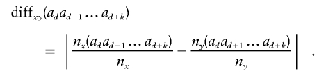
The similarity score of two nodes at level d-1 of the graph is defined as follows. Let n_x be the haplotype count for node x and n_y be the count for node y. For allele a_d at marker d, let n_x(a_d) be the count of those haplotypes that start with the sequences given by the history of node x followed by allele a_d at the marker d; similarly, n_y(a_d) for node y. Now continue, letting n_x(a_da_d+1) be the count for allele a_d+1 at marker d+1 following allele a_d at marker d, following the sequences given by the history of x. Similarly n_x(a_da_d+1a_d+2) and n_y(a_da_d+1a_d+2), and so on. The observed conditional probability difference for the sequence a_da_d+1…a_d+k is

The similarity score for x and y is the maximum over k=0,1,2,3,…,D-d and a_da_d+1…a_d+k of the observed conditional probability difference. The function “Similar” in the work of Ron et al.²⁴ can be used (with slight modification) to efficiently obtain this score.

In general, the algorithm merges nodes x and y if their score is less than a cutoff α (which corresponds to μ/2 in the work of Ron et al.²⁴). I allow α to be a function of the node counts. This is because a node x with small count will have high variability in the observed conditional probability n_x(a_da_d+1…a_d+k)/n_x and hence will be unlikely to have a score less than a fixed cutoff for a node y, even if x and y represent the same conditional probability distribution. Thus, to avoid having the graph with excess numbers of small nodes at each level, with consequent loss of power, the algorithm needs to be less rigorous with small nodes. My choice for α is (n^-1_x+n^-1_y)^1/2.

To justify this choice of cutoff α, assume that the two subtrees (i.e., the nodes x and y with their descendants) are conditionally independent, given the node counts n_x and n_y, and are generated from the same conditional probability distributions (so that these are nodes that should be merged). When an allele sequence ada_d+1…a_d+k is considered, the variance of diff_xy(a_da_d+1…a_d+k) is the variance of n_x(a_da_d+1…a_d+k)/n_x plus the variance of n_y(a_da_d+1…a_d+k)/n_y. This variance is maximized when the true conditional probabilities are one-half, in which case the variance is

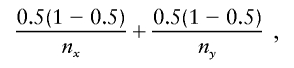which equals

Thus, the maximal standard deviation of diff_xy(a_da_d+1…a_d+k) is 0.5(n^-1_x+n^-1_y)^1/2. Testing of multiple allele sequences adds variability; however, the tests are highly correlated. My choice of cutoff α is twice this SD. In limited simulations comparing subtrees generated from the same conditional probability distributions, I found that the 90th percentile of the similarity score tends to approximate α=(n^-1_x+n^-1_y)^1/2 (data not shown). Thus, a high proportion of subtrees with the same probability distribution will be merged, as they should be.

To ensure that the most strongly supported merges are made, I calculate the score between all pairs of nodes at a level and merge the pair with the lowest score that is below the corresponding cutoff. If a merge occurs, scores are calculated between the new merged node and all other nodes, and I again merge the pair with the lowest score that is below the corresponding cutoff. This process is continued until no more merges are possible.

As an illustration, consider the tree graph shown in figure 2A. I start by considering merging nodes 2.1 and 2.2. The similarity cutoff for these nodes is

I compare the transition probability for edge 1 from each of these nodes and find that it is

for node 2.1 but is

for node 2.2, with a difference of 0.373. Thus, the similarity score for these two nodes is at least 0.373, which exceeds the cutoff, and these two nodes will not be merged.

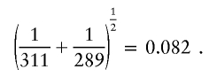
At level 3, I find that the scores for the pairs 3.1/3.2 and 3.2/3.3 exceed the corresponding cutoffs. I describe calculation of the similarity score for nodes 3.1 and 3.3 in detail. The cutoff for these nodes is

The observed conditional probability difference for these nodes and the suffix a₃=1 is

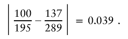The observed probability difference for a₃=2 is also 0.039. When descendants of these nodes are examined, the observed conditional probability difference for suffix a₃=1,a₄=1 is

for a₃=1,a₄=2, it is

and, for a₃=2,a₄=2, it is

Thus, the similarity score for nodes 3.1 and 3.3 is max(0.039,0.039,0.021,0.018,0.039)=0.039, which is less than the cutoff, so the merge can occur. Figure 2B shows the resultant graph. I would continue to look for acceptable merges at level 4 of the new graph (it turns out that there are no further acceptable merges, except for merging all nodes at the final level).

My merging algorithm described above closely follows the algorithm of Ron et al.,²⁴ with two differences. My cutoff for considering merges is a function of the node counts rather than a fixed value. This ensures that low-frequency haplotypes are continually merged into the graph, providing parsimony and ensuring that the graph does not become increasingly spread out over the course of a long sequence of markers. Rather than considering each pair of nodes at a level in turn and merging them if their score is less than the cutoff, I consider all pairs of nodes at once and first merge those pairs that are most similar, subject to the appropriate cutoffs. This ensures that the best merges are made first, rather than allowing borderline merges first that might then rule out other merges that were more strongly supported by the data.

References

- 1.Clark AG (2004) The role of haplotypes in candidate gene studies. Genet Epidemiol 27:321–333 10.1002/gepi.20025 [DOI] [PubMed] [Google Scholar]
- 2.Schaid DJ (2004) Evaluating associations of haplotypes with traits. Genet Epidemiol 27:348–364 10.1002/gepi.20037 [DOI] [PubMed] [Google Scholar]
- 3.Akey J, Jin L, Xiong M (2001) Haplotypes vs single marker linkage disequilibrium tests: what do we gain? Eur J Hum Genet 9:291–300 10.1038/sj.ejhg.5200619 [DOI] [PubMed] [Google Scholar]
- 4.Excoffier L, Slatkin M (1995) Maximum-likelihood estimation of molecular haplotype frequencies in a diploid population. Mol Biol Evol 12:921–927 [DOI] [PubMed] [Google Scholar]
- 5.Zhao JH, Curtis D, Sham PC (2000) Model-free analysis and permutation tests for allelic associations. Hum Hered 50:133–139 10.1159/000022901 [DOI] [PubMed] [Google Scholar]
- 6.Chapman JM, Cooper JD, Todd JA, Clayton DG (2003) Detecting disease associations due to linkage disequilibrium using haplotype tags: a class of tests and the determinants of statistical power. Hum Hered 56:18–31 10.1159/000073729 [DOI] [PubMed] [Google Scholar]
- 7.The International HapMap Consortium (2005) A haplotype map of the human genome. Nature 437:1299–1320 10.1038/nature04226 [DOI] [PMC free article] [PubMed] [Google Scholar]
- 8.Zhao H, Pfeiffer R, Gail MH (2003) Haplotype analysis in population genetics and association studies. Pharmacogenomics 4:171–178 10.1517/phgs.4.2.171.22636 [DOI] [PubMed] [Google Scholar]
- 9.Lin S, Chakravarti A, Cutler DJ (2004) Exhaustive allelic transmission disequilibrium tests as a new approach to genome-wide association studies. Nat Genet 36:1181–1188 10.1038/ng1457 [DOI] [PubMed] [Google Scholar]
- 10.Excoffier L, Laval G, Balding D (2003) Gametic phase estimation over large genomic regions using an adaptive window approach. Hum Genomics 1:7–19 [DOI] [PMC free article] [PubMed] [Google Scholar]
- 11.Templeton AR, Boerwinkle E, Sing CF (1987) A cladistic analysis of phenotypic associations with haplotypes inferred from restriction endonuclease mapping. I. Basic theory and an analysis of alcohol dehydrogenase activity in Drosophila. Genetics 117:343–351 [DOI] [PMC free article] [PubMed] [Google Scholar]
- 12.Tzeng J-Y, Devlin B, Wasserman L, Roeder K (2003) On the identification of disease mutations by the analysis of haplotype similarity and goodness of fit. Am J Hum Genet 72:891–902 [DOI] [PMC free article] [PubMed] [Google Scholar]
- 13.McPeek MS, Strahs A (1999) Assessment of linkage disequilibrium by the decay of haplotype sharing, with application to fine-scale genetic mapping. Am J Hum Genet 65:858–875 [DOI] [PMC free article] [PubMed] [Google Scholar]
- 14.Zöllner S, Pritchard JK (2005) Coalescent-based association mapping and fine mapping of complex trait loci. Genetics 169:1071–1092 10.1534/genetics.104.031799 [DOI] [PMC free article] [PubMed] [Google Scholar]
- 15.Durrant C, Zondervan KT, Cardon LR, Hunt S, Deloukas P, Morris AP (2004) Linkage disequilibrium mapping via cladistic analysis of single-nucleotide polymorphism haplotypes. Am J Hum Genet 75:35–43 [DOI] [PMC free article] [PubMed] [Google Scholar]
- 16.Thomas A, Camp NJ (2004) Graphical modeling of the joint distribution of alleles at associated loci. Am J Hum Genet 74:1088–1101 [DOI] [PMC free article] [PubMed] [Google Scholar]
- 17.Thomas A (2005) Characterizing allelic associations from unphased diploid data by graphical modeling. Genet Epidemiol 29:23–35 10.1002/gepi.20076 [DOI] [PubMed] [Google Scholar]
- 18.Verzilli C, Whittaker J, Stallard N (2005) Graphical models for association mapping in genome-wide studies. Ann Hum Genet 69:774 [Google Scholar]
- 19.Greenspan G, Geiger D (2004) High density linkage disequilibrium mapping using models of haplotype block variation. Bioinformatics 20:i137–i144 10.1093/bioinformatics/bth907 [DOI] [PubMed] [Google Scholar]
- 20.Morris AP, Whittaker JC, Balding DJ (2000) Bayesian fine-scale mapping of disease loci, by hidden Markov models. Am J Hum Genet 67:155–169 [DOI] [PMC free article] [PubMed] [Google Scholar]
- 21.Ron D, Singer Y, Tishby N (1996) The power of amnesia: learning probabilistic automata with variable memory length. Machine Learning 25:117–149 10.1023/A:1026490906255 [DOI] [Google Scholar]
- 22.Eronen L, Geerts F, Toivonen H (2004) A Markov chain approach to reconstruction of long haplotypes. Pacific Symposium on Biocomputing Kamuela, HI, January 6–10 [DOI] [PubMed] [Google Scholar]
- 23.Bühlmann P, Wyner AJ (1999) Variable length Markov chains. Ann Stat 27:480–513 10.1214/aos/1018031204 [DOI] [Google Scholar]
- 24.Ron D, Singer Y, Tishby N (1998) On the learnability and usage of acyclic probabilistic finite automata. J Comp Syst Sci 56:133–152 10.1006/jcss.1997.1555 [DOI] [Google Scholar]
- 25.Kerem B, Rommens JM, Buchanan JA, Markiewicz D, Cox TK, Chakravarti A, Buchwald M, Tsui LC (1989) Identification of the cystic fibrosis gene: genetic analysis. Science 245:1073–1080 [DOI] [PubMed] [Google Scholar]
- 26.Stephens M, Smith N, Donnelly P (2001) A new statistical method for haplotype reconstruction from population data. Am J Hum Genet 68:978–989 [DOI] [PMC free article] [PubMed] [Google Scholar]
- 27.Stephens M, Donnelly P (2003) A comparison of Bayesian methods for haplotype reconstruction from population genotype data. Am J Hum Genet 73:1162–1169 [DOI] [PMC free article] [PubMed] [Google Scholar]
- 28.Daly MJ, Rioux JD, Schaffner SF, Hudson TJ, Lander ES (2001) High-resolution haplotype structure in the human genome. Nat Genet 29:229–232 10.1038/ng1001-229 [DOI] [PubMed] [Google Scholar]
- 29.Abecasis GR, Cherny SS, Cookson WO, Cardon LR (2002) Merlin—rapid analysis of dense genetic maps using sparse gene flow trees. Nat Genet 30:97–101 10.1038/ng786 [DOI] [PubMed] [Google Scholar]
- 30.Mathew CG, Lewis CM (2004) Genetics of inflammatory bowel disease: progress and prospects. Hum Mol Genet 13:R161–168 10.1093/hmg/ddh079 [DOI] [PubMed] [Google Scholar]
- 31.Rioux JD, Daly MJ, Silverberg MS, Lindblad K, Steinhart H, Cohen Z, Delmonte T, et al (2001) Genetic variation in the 5q31 cytokine gene cluster confers susceptibility to Crohn disease. Nat Genet 29:223–228 10.1038/ng1001-223 [DOI] [PubMed] [Google Scholar]
- 32.Carlson CS, Eberle MA, Rieder MJ, Yi Q, Kruglyak L, Nickerson DA (2004) Selecting a maximally informative set of single-nucleotide polymorphisms for association analyses using linkage disequilibrium. Am J Hum Genet 74:106–120 [DOI] [PMC free article] [PubMed] [Google Scholar]
- 33.Scheet P, Stephens M (2006) A fast and flexible statistical model for large-scale population genotype data: applications to inferring missing genotypes and haplotypic phase. Am J Hum Genet 78:629–644 [DOI] [PMC free article] [PubMed] [Google Scholar]
- 34.Hurley JD, Engle LJ, Davis JT, Welsh AM, Landers JE (2005) A simple, bead-based approach for multi-SNP molecular haplotyping. Nucleic Acids Res 32:e186 10.1093/nar/gnh187 [DOI] [PMC free article] [PubMed] [Google Scholar]
- 35.Becker T, Cichon S, Jönson E, Knapp M (2005) Multiple testing in the context of haplotype analysis revisited: application to case-control data. Ann Hum Genet 69:747–756 10.1111/j.1529-8817.2005.00198.x [DOI] [PubMed] [Google Scholar]