Contrast adaptation and representation in human early visual cortex

Summary

The human visual system can distinguish variations in image contrast over a much larger range than measurements of the static relationship between contrast and response in visual cortex would suggest. This discrepancy may be explained if adaptation serves to recenter contrast response functions around the ambient contrast, yet experiments on humans have yet to report such an effect. By using event-related fMRI and a data-driven analysis approach, we found that contrast response functions in V1, V2 and V3 shift to approximately center on the adapting contrast. Furthermore, we discovered that unlike earlier areas, human V4 (hV4) responds positively to contrast changes regardless of the sign, suggesting that hV4 is sensitive to the salience of the change rather than faithfully representing contrast. These findings suggest that the visual system discounts slow uninformative changes in contrast with adaptation, yet remains exquisitely sensitive to changes that may signal important events in the environment.

Introduction

Our visual system is sensitive to many orders of stimulus strength, capable of distinguishing mountains in the mist seemingly as effortlessly as the stripes on a zebra. This ability is all the more amazing given that neurons in the visual pathways are only sensitive to a small range of stimulus strengths. In the cortical visual system, image contrast, the difference between the brightest and darkest part of an image divided by their sum, is the visual property most associated with stimulus strength. Indeed, increasing stimulus contrast makes things more visible and both single unit recordings (c.f. Albrecht and Hamilton, 1982; Anzai et al., 1995; Dean, 1981; Tolhurst et al., 1981) and human imaging (Avidan et al., 2002; Boynton et al., 1999; Boynton et al., 1996; Heeger et al., 2000; Kastner et al., 2004; Logothetis et al., 2001; Tootell et al., 1995) find monotonically increasing activity in the primary visual cortex (V1) with increases in stimulus contrast. However, neurons in V1 do not respond proportionally to all ranges of contrast; they display a sigmoidally shaped contrast response curve (Albrecht and Hamilton, 1982) which is most sensitive to contrast differences in the midrange of the curve and much less to contrasts above or below this range.

Adaptation mechanisms have been proposed as a possible explanation of how the visual system overall can be sensitive to such a wide range of image contrasts while the individual neurons have only limited dynamic range. Prolonged exposure to a stimulus results in a wide range of visual adaptation effects (e.g. Blakemore and Campbell, 1969). In fact, without eye movements, unchanging stimuli appear to fade from perception (Kelly, 1981). These types of perceptual adaptations are paralleled by decreases in firing rates of neurons in V1 (Dean, 1983; Hammond et al., 1985; Movshon and Lennie, 1979; Vautin and Berkley, 1977). If these decreases in neuronal response were generalized to all contrast levels, a response gain decrease, they would be expected to have a detrimental effect on vision, simply reducing sensitivity to all contrasts. However, single-unit experiments in striate cortex of anesthetized cats (Bonds, 1991; Ohzawa et al., 1982; Ohzawa et al., 1985; Sclar et al., 1985), monkey and prosimian V1 (Allison et al., 1993; Carandini et al., 1997; Sclar et al., 1989) and monkey middle temporal area (MT, Kohn and Movshon, 2003) have revealed that adaptation to contrast results in mostly horizontal shifts of contrast response functions. This finding, a contrast gain change, reflects a more beneficial process for vision in that it serves to recenter contrast response curves around the time-averaged contrast level, allowing these neurons to encode contrasts that are relevant to the scene being viewed.

Despite these provocative findings in anesthetized animals, it is not known if these changes occur in the human visual system, let alone whether they are a general mechanism across visual areas. Imaging studies have conflicting reports on whether (Engel and Furmanski, 2001) or not (Kastner et al., 2004) contrast adaptation can be detected in human visual cortex at all, and have not yet tested for how contrast response functions change with adaptation. Outside of V1 only one study (Kohn and Movshon, 2003) has examined how contrast response functions change with adaptation in monkey MT. Despite this lack of physiological evidence in human, psychophysical measurements of contrast discrimination thresholds have been found to change with adaptation in a way that is consistent with contrast gain and not response gain changes (Greenlee and Heitger, 1988). By imaging early visual cortex in awake humans using an event-related functional magnetic resonance imaging (fMRI) technique, we have established that in V1, V2 and V3 there are profound contrast gain changes that are consistent with psychophysics and confer a beneficial effect on human vision.

We also found a basic difference between the response to contrast changes of human V4 (hV4) and earlier visual cortex that has not been reported in either monkey electrophysiology or fMRI experiments; hV4 responded positively to contrast changes regardless of the sign of the change. This result signals a fundamental shift in visual processing between hV4 and earlier areas. While slowly changing or static contrast levels are unlikely to signal biologically relevant events, changes in contrast regardless of whether they are increases or decreases may signal important changes that our visual system should be sensitive to. Contrast adaptation is a process by which neurons adjust to slowly changing or static contrast levels thus reducing our sensitivity to these uninformative features of the visual world. This response property of hV4 that we found is the expected signatures of a process that counterbalances slow adaptation to static contrast by being sensitive to the salience of dynamic changes.

Results

Measurements of contrast response functions with an event-related fMRI paradigm

We measured blood oxygen level-dependent (BOLD) contrast response functions for three different levels of adaptation contrast (6.25, 12.5 and 25%) using an event-related stimulus paradigm (Figure 1, see experimental procedures for details). After an initial 30 sec baseline phase, we adapted the subject for 60 secs, all the time having the subject perform a detection task on the fixation cross to help control fixation and attentional state. We tested contrast response by incrementing or decrementing the contrast by 1 or 2 octaves (an octave being a doubling) for 3 secs. Contrast was the only aspect of the stimulus that we changed during these periods. After each test contrast, we readapted the subject with the adaptation contrast for 8-12 secs. This stimulus paradigm, adapted from electrophysiology experiments (Ohzawa et al., 1982), was used because both the readaptation (or top-up) contrasts and the balancing of contrast increments and decrements serve to keep the time-averaged contrast during the experiment at the adaptation level.

Figure 1.

Visual stimulation paradigm for event-related contrast adaptation experiment (see text for details).

Examination of the timecourse from a representative voxel taken from one subject's retinotopically mapped V1 (see experimental procedures) shows the BOLD response to the various events in our experiment (Figure 2A). The timecourse begins flat with some fluctuations, corresponding to the baseline period of our stimulus paradigm. Soon after we turn on the adaptation stimulus (yellow arrow), the timecourse displays a rapid rise followed by a slower decay. We interpret this decay in response during the adaptation period as a signature of neural adaptation and analyze it in detail in Figure 6. Following this initial adaptation period the timecourse exhibits transient peaks following the times we increased the contrast by 1 or 2 octaves (green and magenta arrows, respectively). Following the times when we decrease the stimulus contrast by 1 or 2 octaves (purple and cyan arrows, respectively), there are transient dips in the timecourse.

Figure 2.

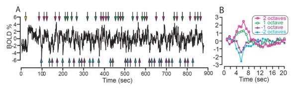
Example timecourse from a single voxel in retinotopically defined V1. A) BOLD response as a function of time from the start of experiment. Yellow arrow marks the time at which the adaptation stimulus was first presented. Green and magenta arrows indicate times at which test contrasts 1 or 2 octaves above the adaptation contrast were presented. Purple and blue arrows mark test contrast presentations 1 or 2 octaves below the adaptation contrast. 0% BOLD is set to the mean level after the 60 sec adaptation period. B) Deconvolved response to each stimulus contrast as a function of time from the beginning of the presentation of each stimulus contrast.

Figure 6.

Analysis of the rate at which adaptation affects BOLD responses. The left column in A, B and C show the response averaged over subjects for the first 60 secs of BOLD response after the adaptation stimulus is first shown, for V1, V2 and V3, respectively. Black arrow indicates the time of initial response that is used to calculate contrast sensitivity shown in the right column (open black squares). The red arrow marks the end of the adaptation period. The open red circles in the right column plot the contrast sensitivity as the average response during the experiment.

To use these transient peaks and dips following contrast increments and decrements as a measure of the contrast response, we first estimated the average response to each contrast using a deconvolution procedure (Figure 2B). This deconvolution procedure, without making any assumptions about the shape of the hemodynamic response, takes a stimulus triggered average and assumes that any overlap in responses results in a linear combination (Boynton et al., 1996; Dale and Buckner, 1997). We found that after an approximately 3 sec delay following increments in stimulus contrast, these hemodynamic responses exhibited a large positive peak followed by a longer lasting negative undershoot, classic features of the hemodynamic response (Kruger et al., 1996). These hemodynamic responses were scaled by the test contrast, displaying a larger response for 2 octaves of contrast as compared to 1 octave (magenta and green curves, respectively). Conversely, when stimulus contrast was transiently decreased the subsequent hemodynamic response displayed a transient decrease in the BOLD response that also scaled with the amount of decrement in stimulus contrast (purple and cyan curves).

We developed a procedure to determine the significance of these types of activations on a voxel-by-voxel basis without recourse to the more usual practice of simply averaging together the response of voxels in a region of interest (ROI) defined by activations from another experiment. We first calculated the amount of variance in the raw timecourse that was accounted for by the hemodynamic responses such as the ones shown in Figure 2B. This value (see experimental procedures for details), r², is equal to 0 if stimulus locked events in the timecourse do not account for any of the variance, and is equal to 1 if these events account for all of the variance. The distribution of r² for all voxels in a volume for one experiment (Figure 3A inset, green bars, mostly obscured by blue bars), shows a broad distribution of values with a mean of 0.09, reflecting the fact that the majority of voxels in the volume are not being activated by our stimulus, and therefore have low r² values. To determine which of these r² values were higher than expected by chance, and therefore significantly activated by our stimulus, we shuffled stimulus times randomly, and recomputed a distribution of r² values (blue bars). An expansion of the tail of the real and randomized distribution (Figure 3A), reveals that the tail of the distribution of real r² values contains values much higher than predicted by chance in the randomized distribution.

Figure 3.

The amount of variance accounted for by stimulus time locked events (r²) is a reliable indicator of activated voxels. A) Distribution of r² values obtained for the real data (green) and when the stimulus times were randomly shuffled (blue). Inset shows the whole distribution for all voxels in the volume, and the main graph shows only the tail of the distribution. Red arrowhead marks the r² cutoff value chosen based on the randomized distribution for this experiment (see text for details). B, C and D show examples of hemodynamic responses from voxels with r² values higher than the cutoff value which are in retinotopically expected areas and show classic hemodynamic responses (same color and symbol convention as Figure 2B).

Maps of r² values (Figure 3, bottom right) with a cutoff chosen based on the randomized distribution (red arrow head, Figure 3A) to produce a false alarm rate probability of p=0.001 validates this measure of activation in two ways. 1) Voxels that have r² values higher than expected by chance were clustered in parts of early visual cortex where they were expected to be based on retinotopy experiments. 2) The hemodynamic response functions of these voxels were all of the classic form (Figure 3B-D). At a cutoff of p=0.001, the image in Figure 3 (cropped to 48×48 voxels) is expected to have 2.3 voxels falsely classified as activated and has 2 obvious false positives located outside the brain (the full image [64×64 voxels) is expected to have 4.1 false positives and has 6).

Using this voxel-by-voxel measure of significance we constructed contrast response functions from the hemodynamic responses of significantly activated voxels (p<0.001). We first calculated the response to the adaptation contrast as the difference between the mean level during the experiment after the adaptation period and the mean level during the baseline period. The rationale for using the mean response was that for the majority of the time during the experiment, the adaptation contrast was presented, and the test stimuli were balanced for contrast increments and decrements, thus making the time-average contrast the same as the adaptation contrast (see below for discussion on possible sources of error). We then fit gamma functions to each one of the estimated hemodynamic functions (Figure 2B) and used the peak of this function as the response to each one of the test contrasts (see experimental procedures for details). These points were then plotted above and below the response to the adaptation contrast. We discarded voxels with a higher than 5% response amplitude as these were likely due to signals from large draining veins and voxels in which the amplitude of the gamma fit was not adequately constrained by the data (variance of the amplitude parameter estimate greater than 50%).

Horizontal shifts of contrast response functions

We plotted contrast response functions in this way for each of the three adaptation contrasts (6.25, 12.5 and 25% contrast, cyan, red and black curves respectively, Figure 4A-C, top row). Each contrast response function shows the average contrast response function (and standard error) constructed from all voxels that showed significant activations (p<0.001) taken from 8 experiments conducted on 5 different subjects (two subjects were tested multiple times). The number of voxels used to construct the curves for 6.25%, 12.5% and 25% adaptation for V1 was 51, 74 and 77, respectively. For V2 there were 34, 46, and 39 voxels and for V3 there were 11, 15 and 22. Examination of these curves reveals that the primary affect of adaptation is to shift the contrast response curves horizontally to the right with higher adaptation contrasts. This trend can be seen for curves generated for V1 (Figure 4A), as well as V2 and V3 (Figure 4B and 4C).

Figure 4.

Contrast response functions for different adaptation levels and in different visual areas. The top row of A, B and C show contrast response functions constructed as detailed in the text for voxels in retiontopically defined V1, V2 and V3 and averaged over all subjects. The bottom three rows show distributions of parameters of fits of contrast response functions performed on a voxel by voxel basis, where the second, third and fourth rows are the distribution of parameters for c₅₀, R_max and offset, respectively (see text for details). Arrows indicate mean values of distributions. As detailed in the text, 0% BOLD is set to the mean response during the baseline period of the experiment.

We next used a voxel-by-voxel analysis to quantitatively examine the shifts in contrast response functions. For this analysis, we fit a sigmoidal function (Albrecht and Hamilton, 1982; Naka and Rushton, 1966) to contrast response functions constructed separately for each activated voxel at each adaptation level (see experimental procedures for equation). In this analysis, we required that a voxel be activated at p<0.001 for all adaptation contrast tested (which was 3 contrasts, except for 2 of the 8 experiments in which we collected only the data for 6.25% and 12.5% adaptation contrast for one and only the 12.5% adaptation contrast for the other). We adjusted three parameters to minimize the squared difference between the curve and the data; the center (c₅₀), the amplitude (R_max) and the offset. These curves fit our data satisfactorily, accounting for 93% of the variance on average. Comparing the distributions of the obtained c₅₀ parameter for different adaptation levels in V1 (2nd row, Figure 4A) shows a systematic shift towards higher values with higher adaptation contrasts. In fact, the mean of the distributions closely track the adaptation contrast for which they were obtained, indicating that the center of the contrast response curves shift near the adaptation contrast. The distribution of R_max (Figure 4A, 3rd row) shows a trend for larger amplitude contrast response functions with higher adaptation levels, but this effect did not generally reach statistical significance (see below). There were no systematic differences in the distribution of offsets (bottom row) for different adaptation levels. The effects of adaptation on these three parameters of the sigmoidal fits to the contrast response functions were qualitatively similar for all three visual areas.

To test the statistical significance of the qualitative results reported above, we used a nested ANOVA in which we tested the difference across adaptation conditions of the data for each voxel nested inside groups collected on different days from different subjects. This analysis confirmed the difference across adaptation conditions of the c₅₀ parameter for V1-V3 (p<0.001), and found no significant difference in means for the offset and R_max parameters (all p>0.7), except for a difference in R_max for V2 (p=0.034). Inter-subject variations were not significant except for the offset parameter for some areas (p=0.0034, p=0.022, p=0.1, V1-V3 respectively) and for the c₅₀ parameter only in V3 (p<0.001, all other p>0.3). These results confirm that the main difference in contrast response functions across adaptation conditions is a shift in the horizontal location (c₅₀) with differences in the amplitude (R_max) reaching borderline significance in one case. Furthermore, there was only a modest amount of inter-subject variation, primarily for the offset parameter.

Horizontal shifts of contrast response functions regardless of voxel selection

We next explored the consequences of changing the voxel selection criteria from the fairly restrictive cutoff used in Figure 4 to one that includes all voxels in the ROI defined from retinotopic mapping. We did this by systematically changing the r² cutoff value for including voxels in the construction of the contrast response functions in V1-V3, using cutoff values of 0.11, 0.10, 0.09, 0.08, 0.05 and 0 (Figure 5, in descending order of color saturation). The final cutoff value corresponds to including all the voxels defined from the retiontopic ROI and included 942, 715 and 633 voxels respectively for V1, V2 and V3. Contrast response functions in V1 and V2 still maintained horizontal shifts with adaptation even when all voxels in the retinotopic ROI were included. However, as more voxels that were not activated by the stimulus were included in the analysis, the contrast response functions become correspondingly more flat. This effect is most pronounced for area V3 which had the least number of activated voxels, flattening the curves to such an extent as to obscure the consequences of adaptation on contrast response.

Figure 5.

Change in contrast response functions with different r² cutoffs. Contrast response functions for V1, V2 and V3 are shown in A, B and C respectively. Curves are constructed with voxels exceeding a cutoff r² value the same as Figure 4 (most saturated colors and thickest lines) and with cutoff values 0.11, 0.1, 0.09, 0.08, 0.05 and 0 (in descending order of color saturation and line thickness). Note that the curve with cutoff of 0 is one that is equivalent to an ROI based approach because it includes all voxels in the ROI.

To quantitatively assess whether these changes in the method of selecting voxels for analysis affect how contrast response functions change with adaptation, we performed a nested ANOVA analysis (similar to the above) on all voxels from V1-V3 defined using the ROI method. Again the difference in c₅₀ was significant for V1-V3 (p<0.001) and no other parameters showed significant differences (p=0.094 for R_max in V1, all other p>=0.4). Inter-subject variations were only significant for the offset parameter for some areas (p<0.001, p=0.23, p=0.050, V1-V3 respectively), the c₅₀ parameter for V3 (p<0.001) and the R_max parameter for V2 (p=0.017, all other p>0.5). These results indicate that our primary observation that the horizontal shift of c₅₀ as a consequence of contrast adaptation in early visual cortex is largely independent of the voxel selection.

Possible sources of error in construction of contrast response functions

In estimating the response to the adaptation contrast we use the mean during the experiment which may be subject to two sources of error. First, though the contrast increments and decrements were balanced on a log scale, the neural responses may not be completely balanced and thus using the mean during the experiment may be a biased measure of the response to the adapting contrast. Second, the high-pass filter used to remove slow drifts in the MR signal, though set to be quite conservative, could have filtered out differences in adaptation level. To test whether these factors might substantially change our results, we recalculated the response to the adaptation contrast, using the timecourse data without any temporal filtering. Also, rather than using the average during the experiment as the response to the adapting contrast, we averaged the last 15 time points acquired in the last 12 secs in the adaptation period, when the response is expected to be near the steady-state level, but not be contaminated by responses to our test stimuli. Using the same nested ANOVA approach as above to examining the new contrast response functions on a voxel-by-voxel basis, we confirmed that this way of constructing the contrast response functions produced equivalent results. Differences in the c₅₀ parameter across adaptation conditions were significant (p<=0.015, V1-V3); the slightly larger p values presumably reflecting the noisier response estimation without filtering. The offsets and R_max parameters were all non-significant across adaptation conditions (p>0.7) except for the R_max parameter for V2 (p=0.033). Employing the full ROI based method and including all voxels regardless of their r² value, again resulted in significant differences for the c₅₀ parameter for all areas (p<=0.011) and non-significance for differences of the offsets and R_max parameters (p>0.3) except for the R_max parameter for V3 (p=0.024).

Timecourse of adaptation

We next examined the timecourse over which neural adaptation to contrast effects the BOLD measurements by examining the initial 60 sec response when the adaptation stimulus was first turned on (starting at yellow arrow, Figure 2A). The average response for voxels in each visual area shows an initial rise in the BOLD signal in response to the adaptation stimulus being turned on, followed by a slower decay as the signal adapts to that contrast. We fit these responses from the time of peak to the end of the adaptation period with a decaying exponential function (solid curves, Figure 6A-C). These functions made reasonable fits to the data accounting for 57-84% of the variance in V1, 50-70% in V2 and 24-63% of the variance in V3. The time constants for the adaptation effect show that this effect has a time scale on the order of tens of secs, with the median time constants from V1-V3 being 14.42 secs (18.03 ± 3.19 secs, mean and standard error).

Previous fMRI experiments have used block design experiments to test contrast sensitivity (Avidan et al., 2002; Kastner et al., 2004; Tootell et al., 1995), in which the response to each contrast is typically measured over many secs. Block design experiments may therefore be more sensitive to the adapted response near the end of adaptation (red arrow, Figure 6A), rather than the initial response to the contrast before adaptation (black arrow, Figure 6A). We examined the difference in contrast sensitivity that these two measures showed, by plotting the initial peak (black squares, Figure 6, right column) and the adapted response taken as the mean during the experiment (red circles). The range of response from the smallest to the largest contrast was much greater for the pre-adaptation data than for the post-adaptation data. For example, the difference in response amplitude for V1 when the stimulus was 6.25% contrast versus 25% contrast was 1.09% of BOLD response. After adaptation, this difference was only 0.28%. Taking the ratio of these values, reveals that the contrast sensitivity was 3.88 times greater before adaptation. Contrast sensitivity measured in this way was 3.10 and 3.37 times greater for V2 and V3, respectively.

Positive responses to contrast decrements in hV4

We found that the responses to contrast decrements in hV4 were fundamentally different from the responses in earlier visual cortex. While earlier visual areas all showed decreases in response when contrast was decremented, voxels in hV4 responded to both contrast decrements and contrast increments with positive responses, a single voxel example of which is shown in Figure 7A. These responses, averaged over voxels, led to flatter contrast response functions than earlier visual areas (Figure 7B), though only a few voxels survived the criteria (p<0.001, on average 4 voxels in each experiment), thus making the curves hard to interpret. When we opened up the criteria to accept false positive probabilities of 0.005, 0.01, 0.02, 0.05, 0.1 (r² from 0.14 to 0.11, Fig 7C, in descending order of color saturation), as well as the full hV4 ROI which had an average of 106 voxels surviving, we found that the contrast response functions began to display a more U, rather than S, shaped curve because of the positive responses to contrast decrements (Figure 7C).To examine these positive responses in detail, we conducted another set of experiments which had two purposes. The first purpose was to increase the yield of voxels in hV4 to confirm that positive responses to contrast decrements was indeed a property of hV4. Our previous experiments were optimized by the slice prescription and surface coil location to examine signals in V1 surrounding the calcarine sulcus. Higher visual areas successively take up less cortical surface (Dougherty et al., 2003) and are further away from the surface coil, thus yielding less voxels for our analysis and consequently the larger error bars in Figures 4 and 7. We therefore reduced our field of view from 24×24 cm² to 20×20 cm² to obtain voxels with smaller inplane resolution (3.125×3.125 mm²). We also tested only two relatively large test contrasts, 87.5% and 12.5%, from an adaptation contrast of 50%, in an effort to elicit large responses. The second, and more fundamental, purpose of this experiment was to test how rapidly contrast decrements had to occur to evoke positive responses from hV4. We therefore had our stimulus modulate as half a period of a sinusoidal modulation of contrast rather than an abrupt change of contrast as we had done before (Figure 8A, insets). These sinusoidal modulations were presented for 12.5, 8.3, 6.25, 4.167 or 3.125 secs. Each block contained a contrast increment and decrement of one length presented at least 12 times each. The stimulus sequence was analogous to the first experiment (Figure 1), except that the initial adaptation period was 40 secs.

Figure 7.

Responses to contrast decrements in hV4 were positive rather than negative. A) Hemodynamic responses to test contrasts for a representative voxel in hV4 (same conventions as Figure 2B). B shows the average contrast response function constructed for voxels in hV4 with the same criteria as Figure 4 (B, p<0.001). C shows curves constructed from voxels with p < 0.001, 0.005, 0.01, 0.02, 0.05, 0.10 and for the full ROI (r² >= 0.136, 0.128, 0.124, 0.120, 0.114 and 0.109, and 0 respectively) in descending order of color saturation and line thickness.

Figure 8.

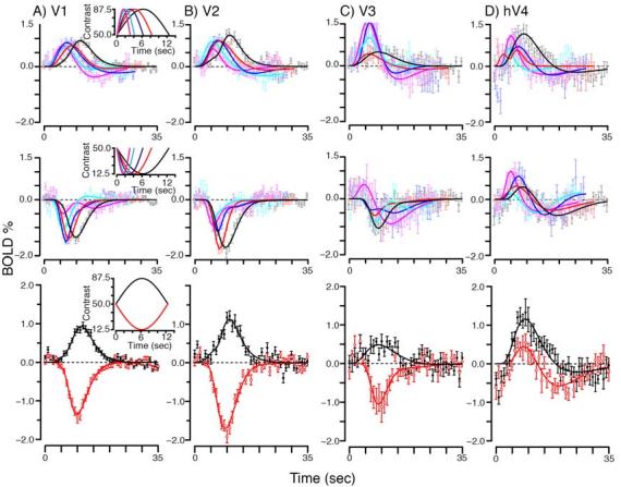
Positive responses to contrast decrements in hV4 examined with different stimulus lengths. Each column represents the responses found to contrast increments (top row) or contrast decrements (middle row) presented as one half period of a sinusoidal modulation. Magenta, cyan, blue, red and black traces and symbols represent the responses for 3.125, 4.167, 6.25, 8.3 and 12.5 secs of stimulus duration, respectively. Insets in the first column display stimulus types. Bottom row replots the response to the longest stimulus duration (12.5 secs) for both contrast increments (black) and decrements (red), to facilitate comparison between the two (see text for details).

As expected, we found that V1-V3 responded with positive responses to contrast increments (top row, Figure 8A-C) and negative responses to contrast decrements (middle row). These positive and negative responses scaled appropriately with the stimulus lengths (magenta, cyan, blue, red and black traces, in length order). In contradistinction, hV4 exhibited positive responses regardless of whether the contrast was incremented (top row, Figure 8D) or decremented (middle row). We note that, one response (to the shortest length) in V3 (magenta curve, middle row, Figure 8C) showed an early positive response to a contrast decrement. However, the error bars on the positive portion of this response suggest caution in interpretation without further replication.

One puzzling aspect of the positive response in hV4 to contrast decrements is that as contrast is decremented, the visual input to hV4 from V1-V3 is decreased and would be expected to result in a lower response in hV4. By examining the timecourse of the response in hV4, we found evidence that the initial positive hV4 response to contrast decrements is followed by a slower negative response. This can be appreciated by directly comparing the positive and negative responses (bottom row, Figure 8D) for the longest duration (12.5 sec) contrast change (solid line is a difference of gamma fit to the data, see experimental procedures). The response to contrast decrements (red trace), starts out positive, but then ends with a large negative component. In principle, this negative response could be the post-undershoot (Kruger et al., 1996) component of the hemodynamic response, attributable to a lagged blood volume effect (Buxton et al., 2004; Mandeville et al., 1998) and not a decrease in neural firing. If this were the case, we would expect this negative portion of the response to scale with the initial positive response. In particular, the negative component should be the same magnitude or smaller than the negative component of the response to the contrast increment (black trace) which has a larger initial positive response. That it is not, suggests that the negative component of the response to contrast decrements is not simply a post-undershoot, but a decrease in the underlying neural response that occurs after the initial increase to the contrast decrement. For all 5 stimulus lengths, the negative component of the response to the contrast decrements was more negative than the positive response; on average the difference in the minimum of the fits was 0.28% of BOLD response (p<0.01, different from 0, student's t-test).

Discussion

We measured contrast response functions in human early visual cortex after contrast adaptation and found that these curves displayed primarily horizontal shifts that nearly recenter these curves on the adapting contrast. While these horizontal shifts of contrast response functions were very evident for V1-V3, we found that hV4 showed a qualitatively different response to contrast decrements. Earlier cortex showed positive responses to contrast increments and negative responses to contrast decrements, but hV4 showed positive responses regardless of whether contrast was incremented or decremented.

Methodology

To test for adaptation effects on contrast response functions, it was imperative to use event-related imaging techniques to have test stimuli that were short enough to measure the contrast response without significantly altering the adaptation state itself. We implemented an analysis technique that did not make assumptions about the shape of the hemodynamic response and used the event related responses themselves to determine activations. We believe this technique was critical for our measurements not simply because it gave us the ability to test contrast sensitivity without inducing significant adaptation, but because it allowed us to make measurements on a voxel-by-voxel basis. Event-related experiments often rely on a ROI defined using a separate set of localizer experiments and average together the responses of all identified voxels to calculate the response in the event-related experiment. This tends to include some voxels not activated in the event-related experiment, thus reducing the signal. Our technique measures the activity in the event-related experiment itself and therefore allows us to analyze only voxels that are significantly activated in the paradigm, thus improving the quality of the signal we measure.

Possible mechanisms of adaptation

Adaptation is unlikely to be simply a passive consequence of a decreased ability to maintain high firing rates due to a lack of metabolic capacity, i.e. neural fatigue, as it confers beneficial properties on visual processing. Moreover, adaptation is associated with a tonic hyperpolarization in V1 neurons (Carandini and Ferster, 1997; Sanchez-Vives et al., 2000b) that may be attributable to synaptic depression (Adorjan et al., 1999; Chance et al., 1998; Finlayson and Cynader, 1995) or Ca²⁺ and Na⁺ activated K⁺ currents (Sanchez-Vives et al., 2000a), suggesting that it is an active process regulated by the cortex. Our data may suggest that this active process of adaptation also serves to reset the metabolic baseline; producing less metabolic demands for static stimuli, and thus providing reserve ability to sustain higher activity necessary to encode changes in visual scenes. This suggestion is based on the indirect relationship between the BOLD signal and changes in metabolism; the part of the BOLD signal that we use in our analysis is dominated by a signal induced by a change in cerebral blood flow (CBF) that overcompensates for changes in the cerebral metabolic rate of oxygen consumption (CMRO₂) (Buxton et al., 2004). However, CBF and CMRO₂ are usually coupled (Hoge et al., 1999), suggesting that the overall change in BOLD signal that we measure is positively correlated with metabolic demands. If adaptation is caused by an active hyperpolarization of cortical activity, this process is metabolically efficient, requiring less metabolic resources than simply maintaining activity related to stimuli that do not change.

Early experiments with contrast adaptation found that contrast gain shifts were present at the level of striate cortex but not at the inputs from the lateral geniculate nucleus (Bonds, 1991; Ohzawa et al., 1982), suggesting that the adaptation in the BOLD signal we measure is not due to feedforward synaptic input, but rather neuronal firing and recurrent feedback. However, more recent findings have suggested that contrast adaptation may not be specific to cortical processing, but may also occur in the LGN (Shou et al., 1996), particularly in the magnocellular division (Solomon et al., 2004) as well as the retina (Chander and Chichilnisky, 2001; Smirnakis et al., 1997). While it would be interesting to know if our stimulus conditions give rise to contrast gain changes in the human LGN, our slice prescription and imaging procedures were optimized to record signals in V1 and therefore would require further retooling and optimization to record useful signals from the LGN (Chen et al., 1998; Kastner et al., 2004).

Relation to previous experiments

While anesthetized cat experiments (Bonds, 1991; Ohzawa et al., 1982; Ohzawa et al., 1985; Sclar et al., 1985) have described contrast gain changes with adaptation to contrast, some human imaging experiments (Kastner et al., 2004) have not found contrast adaptation, while others (Engel and Furmanski, 2001) have. Our experiments have uncovered robust contrast gain changes that very nearly center contrast-response functions on the adapting contrast, closely mirroring the cat data in terms of contrast gain (Ohzawa et al., 1982) and rate of adaptation (Albrecht et al., 1984). While individual neurons in single-unit studies may show a range of susceptibility to adaptation (Sclar et al., 1989), our measurements are sensitive to the activity of large populations of neurons and therefore indicate that on the whole, contrast gain changes shift contrast response to the range that is functionally beneficial. Previous block design imaging experiments (Kastner et al., 2004), which have compared contrast response functions measured with ascending versus descending contrasts, may not have been as sensitive to adaptation changes as event-related studies (this study and Engel and Furmanski, 2001). Changes in contrast response functions measured with BOLD imaging have been noted in surround suppression experiments (Zenger-Landolt and Heeger, 2003), sharing some similarities with the effect we find with adaptation. However, surround suppression induces more response-gain changes and is likely to be mediated by neurons with different receptive field locations. Finally, the contrast gain changes that we have documented are closely paralleled to psychophysical measurements (Greenlee et al., 1991; Greenlee and Heitger, 1988). These psychophysical findings demonstrate that adaptation to a high contrast results in lowering of contrast discrimination thresholds at high contrast at the expense of discrimination at lower contrasts, just as would be predicted by our findings.

Our results have implications for previous measurements of contrast sensitivity using functional imaging techniques. Functional imaging experiments have typically used longer block designs to improve signal to noise ratio by averaging responses over longer periods of time. However, the time constants of adaptation that we found, with a median of ∼14 secs, indicate that long blocks of stimulation may confound contrast sensitivity with adaptation. In fact, our measurements of contrast sensitivity before and after adaptation, indicate that block design experiments (depending on the length of the block) could, in the limit, underestimate contrast sensitivity by more than three times. Accurate measurements of contrast sensitivity are particular important for studies that wish to relate BOLD measurements to behavior (Boynton et al., 1999; Zenger-Landolt and Heeger, 2003) or to level of neural activity (Heeger et al., 2000). Moreover, when comparing contrast sensitivity across areas (Avidan et al., 2002), differences in adaptation rates may result in misestimation of contrast sensitivities. Adaptation rates have been found to increase with higher order areas (Tolias et al., 2001), suggesting that decreases in contrast sensitivity may in part be due to differences in rates of adaptation.

Functional baseline

Our method for constructing contrast response functions relies on both steady-state and transient BOLD responses, thus we implicitly assume that it is valid to combine these two types of measurements. If the hemodynamic response itself undergoes adaptation, our results may overestimate the amount of neural adaptation that has occurred. However, this is generally not thought to be the case (Bandettini et al., 1997). Moreover, the time constants of the adaptation we observed are very similar to those reported from single-unit studies, thus supporting our interpretation of neural and not hemodynamic adaptation.

Our study also uses both positive and negative BOLD responses which may not be directly comparable. Indeed, we have noted some differences in temporal dynamics of the two (Gardner et al., 2005). However, there is no evidence that the magnitude of these positive and negative BOLD responses correspond to different magnitude changes of neural response. Even if this were to be the case, differences in the magnitude of positive and negative BOLD responses would be expected to affect all of our contrast response functions, thus changing the shape of the curves but not the horizontal shift with adaptation.

The comparison of transient to sustained baseline responses is not limited to our study or even adaptation studies in general, but is ubiquitous among functional imaging studies. For example, testing the response to a visual stimulus from a neutral background assumes that the neutral background gives the natural baseline response for visual cortex, an assumption that is debatable (Gusnard and Raichle, 2001). While studies have manipulated the hemodynamic baseline pharmacologically (Hyder et al., 2002) or through hypercapnia (Cohen et al., 2002) to examine the consequences for transient responses, it is not clear if these artificial interventions are relevant to natural changes in baseline. Our results provide a functionally relevant way to change baseline and therefore suggest that the baseline for visual cortex is an adaptive state, controlled in part by the cortex itself.

Contrast representation in hV4 vs V1-V3

Our experiments picked up a fundamental difference between the response of V1-V3 and hV4 to contrast decrements; while earlier areas responded with increases and decreases in BOLD response to contrast increments and decrements respectively, hV4 responded with increased responses to both increments and decrements of contrast (c.f. Engel, 2005). Only at a longer time scale did hV4 decrease its response to decrements in stimulus contrast. Previous lesion experiments have implicated monkey V4 as being especially important for detecting stimuli like decrements in contrast that are less salient than neighboring distractors (Schiller and Lee, 1991)—a task that shows benefits with spatially directed attention (Braun, 1994). Our results may be another signature of the same phenomenon, suggesting that hV4 does not faithfully represent contrast as much as earlier areas, but signals the salience of changes in stimulus contrast.

This result for hV4 is not predicted by previous reports of task-related or attentional modulations in human visual cortex (Pessoa et al., 2003). We controlled attention across presentations of different stimulus type, by having the subjects perform a detection task on the fixation cross throughout the experiment. Even still, abrupt changes in stimulus contrast can automatically grab spatial attention (Jonides and Yantis, 1988) and therefore our results could be associated with this type of transient attention. If it is, it is very different than previous reports of modulations due to task contingencies and sustained attention (Brefczynski and DeYoe, 1999; Gandhi et al., 1999; Somers et al., 1999; Tootell et al., 1998; Watanabe et al., 1998) or transient attention (Liu et al., 2005) which have found large effects in early visual cortex often including V1.

Our findings indicate that earlier visual areas do not show positive responses to contrast decrements, the way hV4 does, suggesting that this visual function emerges in hV4 itself. This type of response which does not distinguish between increments and decrements in contrast may be functionally analogous to the way that complex cells in V1 signal both increments and decrements of luminance. It could in principle be achieved through rectification and summing or squaring of the output of neurons in earlier visual areas that show signed responses to contrast increments and decrements. However, unlike luminance, there are no known analogous cell classes to on- and off-type LGN cells that respond with positive responses to contrast increments and decrements respectively. It therefore seems likely that the synaptic mechanisms in hV4 that give rise to these responses is qualitatively different than those of V1 neurons, and may involve cortical feedback mechanisms rather than feedforward mechanisms.

This property that distinguishes hV4 from early visual cortex could be used as a functional marker that could help in defining the hierarchy of human visual areas (Hadjikhani et al., 1998; McKeefry and Zeki, 1997; Wandell et al., 2005; Zeki et al., 1998; Zeki et al., 1991) and aid in determining homologies to the monkey hierarchy.

Conclusion

In conclusion, our results demonstrate contrast gain changes in human cortex that roughly serve to center contrast response functions on the adaptation contrast, thus allowing neurons with limited dynamic range to represent the much larger range of contrasts present in the visual world. Contrast gain changes like what we have measured are a slow process which adjusts sensitivity of neurons to unchanging and therefore less informative aspects of visual scenes. We have also discovered a complementary mechanism which is not present in visual areas earlier than hV4. This mechanism is very sensitive to changes in contrast, regardless of the sign of the change. Differences in time scale of changes in stimulus contrast can be an informative cue as to their behavioral relevance. Things that change rapidly signal events in the world that may be dangerous, like a predator, or potentially rewarding, like a prey. Slow changes may be due to lighting differences or otherwise uninformative aspects of the environment. Our study demonstrates two mechanisms in the human visual system, one that makes contrast gain adjustments so as to be insensitive to slow changes in overall contrast, and another that is sensitive to rapid changes in contrast that could signal informative events.

Experimental Procedures

Human Subjects

We studied the occipital visual cortex of five healthy male subjects, two of which are authors (ages 29-41). All procedures were approved in advance by the RIKEN Functional MRI Safety and Ethics Committee and subjects gave prior written informed consent before each experiment.

Imaging Hardware

All experiments were conducted on a Varian Unity Inova 4 Tesla whole-body MRI system (Varian NMR Instruments, Palo Alto, CA) equipped with a Magnex head gradient system (Magnex Scientific Ltd., Abingdon, UK). High-resolution three-dimensional T1-weighted anatomical MR images were scanned with a bird-cage radio-frequency (RF) coil or a transverse electromagnetic RF coil. A 5 inch transmit/receive butterfly quadrature RF surface coil was used to acquire functional (T2*-weighted) and anatomical (T1-weighted) images during the contrast adaptation experiments.

Rigid head motion was restricted by requiring subjects to use a bite-bar and by firmly padding the head into the head-rest with spongy rubber. Two pressure sensors placed around the subject's head were used to monitor any head motion during the experiment. The subject's heartbeat was monitored with a pulse oximeter, and respiration was monitored with a pressure sensor. Both signals were recorded along with the timing of RF pulses for later corrections of physiological fluctuations.

Visual Stimulation

Visual stimuli were generated on a Macintosh computer using the Psychophysics Toolbox (Brainard, 1997; Pelli, 1997) running on Matlab 5.2.1 (Mathworks, Natick, MA) and were displayed to the subject via an optic fiber goggle system (Silent Vision binocular glasses, Avotec Inc., Jensen Beach, FL) which subtended 30° by 23° of visual angle. Subjects adjusted two refractive correction lenses on the goggle system to achieve corrected-to-normal vision. The luminosity of the brightest white color achievable on the goggles was ∼4 Lux and the darkest black color was ∼0.5 Lux (measured with Extech 403125 Light ProbeMeter, Extech Instruments Co., Waltham, MA), resulting in a contrast of 8. Gamma of the goggles was measured with a psychophysical procedure and corrected using routines from the Psychophysics Toolbox.

The stimulus sequence began with 30 secs of fixation in which the subject viewed a gray screen (Figure 1). To help the subject maintain fixation and evenly allocate attention we had the subject do a moderately demanding detection task on the fixation cross throughout the whole experiment. Every 3-5 secs the fixation cross would turn red for 100 ms, and the subject was required to report that event with a button press. We nevertheless monitored and recorded the subject's eye positions using an eye tracker built in the goggle system with an SMI iView software package (SensoMotoric Instruments, Boston, MA). The off-line analysis of the eye positions confirmed that the subject maintained fixation throughout the experiment. After the initial baseline period, an adaptation stimulus was presented for 60 secs. The stimulus consisted of four 8 deg diameter stimuli placed 7 deg diagonally away from the fixation point. The checkerboards had a checker size of 1 deg and flickered at 7.5 Hz. We split the stimuli into four quadrants, avoiding the fovea and the horizontal and vertical meridians so as to aid with later retinotopic mapping. The stimulus contrast defined as the difference in luminance between the bright and dark squares divided by the sum (and multiplied by 100) was set to an adaptation level of 6.25, 12.5 or 25%. After this initial adaptation period, we would randomly interleave test contrast stimuli which had a different contrast but were otherwise identical to the adaptation stimulus. We tested contrast that were 1 or 2 octaves above or below the adaptation contrast (an octave being a double of contrast). These test contrasts were presented in random order and we ran the full experiment for approximately 16 minutes so as to get 15 or more repeats of each test contrast. In between each test contrast we presented the adaptation contrast again for 8-12 secs to maintain the adaptation level.

Imaging Parameters

We collected 8 slices perpendicular to the calcarine sulcus. Anatomical images were collected with a four segment T1-weighted FLASH sequence. Functional images were acquired with a two segment centric ordered EPI sequence which had a volume TR of 0.8 secs (100 ms per slice) and a TE of 25 ms. Functional images had a slice thickness of 4 mm and an in-plane resolution of either 3.75 x 3.75 mm² (field of view [FOV] = 24×24 cm², matrix size = 64×64) for the contrast adaptation experiments (Figures 1-7) or 3.125 × 3.125 mm² (FOV = 20×20 cm², matrix size = 64×64) for the contrast sinusoid experiments (Figure 8). Longitudinal magnetization was allowed to reach steady state before EPI images were collected. A reference scan of a full volume without phase encoding was taken at the beginning of the sequence and used to correct for phase errors (Bruder et al., 1992). The first echo in each segment was acquired as a navigator echo which was used to correct intersegment phase and amplitude variations (Kim et al., 1996).

Data Processing and Analysis

After the EPI images were reconstructed, physiological (cardiac and respiratory) fluctuations were further removed from the time series using a retrospective estimation and correction method with the pulse and respiration data recorded during image acquisition (Hu et al., 1995). We then applied a motion correction algorithm (Maas et al., 1997) to correct for any residual translational motion. Both physiological and motion corrections were performed in k space. A high-pass filter was then used to remove linear trends. This filter was set to have a cutoff frequency of 0.004 cycles/sec but to retain the DC level. This frequency was chosen so as not to interfere with stimulus related responses in the time series. The event-related responses were of sufficiently high frequency to be largely unaffected by this filter. However, the initial decay that we analyze in Figure 6 could have been affected (i.e. the high pass filter could accentuate the exponential decay we report in the signal). Analysis of time-courses without application of the filter resulted in qualitatively similar exponential decay and did not substantially affect our results. We therefore opted to use the filter, because without it the event-related analysis would be strongly biased by the slow drifts caused by noise. All further analyses after these preprocessing steps were preformed with custom-built software in Matlab 6.5 (Mathworks, Natick, MA).

We computed estimated hemodynamic response functions for each stimulus in individual voxels without making any assumptions about the shape of the hemodynamic response. We did this by assuming the following model of the BOLD timecourse in our experiment, in block matrix format:

$$\text{Equation 1}:\left[S_1{S}_2\dots S_n\right]\times {\left[H_1{H}_2\dots H_n\right]}^T+\text{noise}={\left[\text{BOLD}\right]}^T$$

S_i is the stimulus convolution matrix for the i^th stimulus. Each S_i has dimensions M×N where M is the number of time points in the timecourse and N is the number of time points for which we calculate the estimated hemodynamic response (We calculate 20 secs of response, which for a TR of 0.8 secs contains 25 time points). Each H_i is a 1×N array of the unknown hemodynamic response to the i^th stimulus. T is the transpose operation. Noise is assumed to be zero-mean Gaussian. BOLD is a 1×M array which contains a mean subtracted time series for the voxel. We then computed the hemodynamic responses (H_i) to each stimuli at each voxel that minimized the squared error between the left and right sides of equation 1 by applying the normal equations to the BOLD response for that voxel. We chose to randomize interstimulus times so that in addition to sampling different combinations of responses to the different stimuli, we would also sample different temporal combinations of responses (Burock et al., 1998). We also attempted to reduce estimation errors of the hemodynamic response due to violations of temporal linearity, by separating stimuli in time by a longer time interval than the main positive part of the hemodynamic response (i.e. 8-12 secs). Raw imaging values were converted to percent modulations by dividing the timecourses by the average response during the baseline period. 0% modulation was set to the mean during the experiment.

We developed a statistical analysis procedure in which we could use the event-related responses in each individual voxel without reference to a separate localizer to evaluate activation. Our analysis asks what percent of the variance in the BOLD response could be accounted for by events that are time-locked to stimulus presentations. We did this by first generating an estimated timecourse by convolving the estimated hemodynamic responses with the stimulus convolution matrices. We then computed the amount of variance in the original timecourse that is accounted for by this estimate (r²):

$$\text{Equation 2}:r^2=1-\frac{\mathrm{var}\mathit{iance}\left(\mathit{residual}\right)}{\mathrm{var}\mathit{iance}\left(\mathit{original}\right)}$$

Where the residual was the difference between the estimated timecourse and the original timecourse.

To estimate the statistical significance of a particular value of r² we used a randomization procedure. We shuffled the stimulus times so that they were no longer time-locked to stimulus events. We then recalculated hemodynamic responses for every voxel in the volume according to the least-squares solution of Equation 1 and then recalculated r² values. We took the distribution of r² values calculated in this way to represent the distribution of r² values that would be expected by chance correlations of noise with stimulus times. When we compared the distributions of r² values calculated in this way to the real r² distribution and found that the tails of the distribution were different. The real r² distribution had many larger values of r² than the randomized distributions. These values of r² we took to be significantly activated. We could then get p-values based on the randomized distribution by finding a cutoff that included only a desired amount of noise voxels, for example, 0.1%, by picking the r² value of the voxel that ranked as the 99.9% highest r² value in the randomized distribution. This would insure that in the real data, with a cutoff chosen in this way that we could expect to have 0.1% of the voxels that were deemed activated by the stimulus to actually be simply noisy voxels with spurious correlations with the stimulus times (Figure 3). The cutoff value was determined for each scan individually.

To quantify the magnitude of activation to each stimulus type, we estimated parameters of a gamma function of the following form to the data:

$$\text{Equation 3}:\mathrm{A}\frac{{\left(\frac{t-\mathit{lag}}{\tau }\right)}^{n-1}{e}^{-\frac{t-\mathit{lag}}{\tau }}}{\tau (n-1)!}$$

Where A is the amplitude, n is a shape parameter that was allowed to take on integer values from 4 to 6, τ was another shape parameter, roughly corresponding to the width of the response and was allowed to take on values from 0.5 to 2 secs. The lag value controlled when the gamma function began relative to stimulus onset and took on values ranging from 0 to 4 secs. When (t-lag) took on negative values, the function was assumed to give a value of 0. The maximum value of these gamma functions was taken as a measure of the peak response. A difference of gamma functions (Equation 3), in which the second gamma function was allowed to have τ values between 0.5 and 4 secs, and the lag was allowed to take on values from 2-8 secs was used to capture the delayed negative response of the hemodynamic function.

We fit the parameters of the gamma functions by first making an estimated timecourse in which each stimulus occurrence was replaced by a gamma function (for each stimulus type we used a separate set of parameters). Any overlap in the gamma functions from one stimulus to the next was assumed to sum linearly. We then used LevenbergMarquardt optimization to find the parameters of each gamma function that minimzed the mean squared difference between the estimated timecourse and the actual timecourse. Our stimulus presentation times were intentionally not synched to volume acquisition so that on different stimulus presentations, different time points relative to the stimulus onset would be sampled. Furthermore, our multi-shot protocol was not interleaved across slices so that we could use the actual time of slice acquisition instead of the volume TR to get better time resolution of the response.

We fit contrast response curves with the following equation:

$$\text{Equation 4}:\mathrm{Re}\mathit{sponse}=R_{\max }\frac{{\mathit{contrast}}^n}{{\mathit{contrast}}^n+{c_{50}}^n}+\mathit{offset}$$

Where R_max is the maximum amplitude and c₅₀ is the contrast at which the curve reaches half height, and n controls the steepness of the curve. We set n to 2, so as to avoid overfitting of the data. Offset was allowed to take on any value while R_max and c₅₀ were allowed to only take on positive values. 0% BOLD for the contrast response functions is taken as the response during the baseline condition.

To estimate the rate of adaptation, we minimized the squared error between a decaying exponential equations of the following form and the initial portion of the response:

$$\text{Equation 5}:{\mathit{Ae}}^{-\frac{t}{\tau }}+\mathit{offset}$$

Where A is the amplitude and τ is the time constant.

Retinotopy

We segmented our data into ROIs for different visual areas by running a retinotopy scan in which we mapped the horizontal and vertical meridians (c.f. Engel et al., 1994; Sereno et al., 1995). We did this with an event-related stimulus paradigm similar to the one we used for the contrast adaptation experiments. We presented 45 deg wide wedges of flickering checkerboards either along the horizontal or vertical meridian (randomly interleaved) for 3 secs. Each presentation of the stimulus was followed by 4-8 secs of a gray field. We computed hemodynamic responses and mapped the meridians by displaying the difference between the peak response to the horizontal or vertical stimuli. We then marked the visual regions as areas that extended from one meridian to the next meridian along the gray matter and marked these using the software package BrainVoyager. We defined V1-V3 in both dorsal and ventral aspects, and since we did not see significant differences between the dorsal and ventral V1-V3 areas (though our slice positioning tended to oversample the ventral areas), we combined data from the two. Human V4 (hV4) was defined as the ventral visual area that continues laterally from V3. This area, typically located on the medial lip of the collateral sulcus but avoiding the depth of the sulcus, corresponds mostly to V4v defined in other retinotopic studies (Hadjikhani et al., 1998; Sereno et al., 1995). These data were then registered with a 3D anatomical image collected from the whole brain. Each functional dataset was also registered with this 3D anatomical view of the brain. We determined whether a voxel was in a particular visual area in a strict fashion by requiring that the voxel overlapped with the ROI for that visual area and not with any other ROI.

References

- Adorjan P, Piepenbrock C, Obermayer K. Contrast adaptation and infomax in visual cortical neurons. Rev Neurosci. 1999;10:181–200. doi: 10.1515/revneuro.1999.10.3-4.181. [DOI] [PubMed] [Google Scholar]
- Albrecht DG, Farrar SB, Hamilton DB. Spatial contrast adaptation characteristics of neurones recorded in the cat's visual cortex. J Physiol. 1984;347:713–739. doi: 10.1113/jphysiol.1984.sp015092. [DOI] [PMC free article] [PubMed] [Google Scholar]
- Albrecht DG, Hamilton DB. Striate cortex of monkey and cat: contrast response function. J Neurophysiol. 1982;48:217–237. doi: 10.1152/jn.1982.48.1.217. [DOI] [PubMed] [Google Scholar]
- Allison JD, Casagrande VA, Debruyn EJ, Bonds AB. Contrast adaptation in striate cortical neurons of the nocturnal primate bush baby (Galago crassicaudatus) Vis Neurosci. 1993;10:1129–1139. doi: 10.1017/s0952523800010233. [DOI] [PubMed] [Google Scholar]
- Anzai A, Bearse MA, Jr., Freeman RD, Cai D. Contrast coding by cells in the cat's striate cortex: monocular vs. binocular detection. Vis Neurosci. 1995;12:77–93. doi: 10.1017/s0952523800007331. [DOI] [PubMed] [Google Scholar]
- Avidan G, Harel M, Hendler T, Ben-Bashat D, Zohary E, Malach R. Contrast sensitivity in human visual areas and its relationship to object recognition. J Neurophysiol. 2002;87:3102–3116. doi: 10.1152/jn.2002.87.6.3102. [DOI] [PubMed] [Google Scholar]
- Bandettini PA, Kwong KK, Davis TL, Tootell RB, Wong EC, Fox PT, Belliveau JW, Weisskoff RM, Rosen BR. Characterization of cerebral blood oxygenation and flow changes during prolonged brain activation. Hum Brain Mapp. 1997;5:93–109. [PubMed] [Google Scholar]
- Blakemore C, Campbell FW. On the existence of neurones in the human visual system selectively sensitive to the orientation and size of retinal images. J Physiol. 1969;203:237–260. doi: 10.1113/jphysiol.1969.sp008862. [DOI] [PMC free article] [PubMed] [Google Scholar]
- Bonds AB. Temporal dynamics of contrast gain in single cells of the cat striate cortex. Vis Neurosci. 1991;6:239–255. doi: 10.1017/s0952523800006258. [DOI] [PubMed] [Google Scholar]
- Boynton GM, Demb JB, Glover GH, Heeger DJ. Neuronal basis of contrast discrimination. Vision Res. 1999;39:257–269. doi: 10.1016/s0042-6989(98)00113-8. [DOI] [PubMed] [Google Scholar]
- Boynton GM, Engel SA, Glover GH, Heeger DJ. Linear systems analysis of functional magnetic resonance imaging in human V1. J Neurosci. 1996;16:4207–4221. doi: 10.1523/JNEUROSCI.16-13-04207.1996. [DOI] [PMC free article] [PubMed] [Google Scholar]
- Brainard DH. The Psychophysics Toolbox. Spat Vis. 1997;10:433–436. [PubMed] [Google Scholar]
- Braun J. Visual search among items of different salience: removal of visual attention mimics a lesion in extrastriate area V4. J Neurosci. 1994;14:554–567. doi: 10.1523/JNEUROSCI.14-02-00554.1994. [DOI] [PMC free article] [PubMed] [Google Scholar]
- Brefczynski JA, DeYoe EA. A physiological correlate of the ‘spotlight’ of visual attention. Nat Neurosci. 1999;2:370–374. doi: 10.1038/7280. [DOI] [PubMed] [Google Scholar]
- Bruder H, Fischer H, Reinfelder HE, Schmitt F. Image reconstruction for echo planar imaging with nonequidistant k-space sampling. Magn Reson Med. 1992;23:311–323. doi: 10.1002/mrm.1910230211. [DOI] [PubMed] [Google Scholar]
- Burock MA, Buckner RL, Woldorff MG, Rosen BR, Dale AM. Randomized event-related experimental designs allow for extremely rapid presentation rates using functional MRI. Neuroreport. 1998;9:3735–3739. doi: 10.1097/00001756-199811160-00030. [DOI] [PubMed] [Google Scholar]
- Buxton RB, Uludag K, Dubowitz DJ, Liu TT. Modeling the hemodynamic response to brain activation. Neuroimage. 2004;23(Suppl 1):S220–233. doi: 10.1016/j.neuroimage.2004.07.013. [DOI] [PubMed] [Google Scholar]
- Carandini M, Barlow HB, O'Keefe LP, Poirson AB, Movshon JA. Adaptation to contingencies in macaque primary visual cortex. Philos Trans R Soc Lond B Biol Sci. 1997;352:1149–1154. doi: 10.1098/rstb.1997.0098. [DOI] [PMC free article] [PubMed] [Google Scholar]
- Carandini M, Ferster D. A tonic hyperpolarization underlying contrast adaptation in cat visual cortex. Science. 1997;276:949–952. doi: 10.1126/science.276.5314.949. [DOI] [PubMed] [Google Scholar]
- Chance FS, Nelson SB, Abbott LF. Synaptic depression and the temporal response characteristics of V1 cells. J Neurosci. 1998;18:4785–4799. doi: 10.1523/JNEUROSCI.18-12-04785.1998. [DOI] [PMC free article] [PubMed] [Google Scholar]
- Chander D, Chichilnisky EJ. Adaptation to temporal contrast in primate and salamander retina. J Neurosci. 2001;21:9904–9916. doi: 10.1523/JNEUROSCI.21-24-09904.2001. [DOI] [PMC free article] [PubMed] [Google Scholar]
- Chen W, Kato T, Zhu XH, Strupp J, Ogawa S, Ugurbil K. Mapping of lateral geniculate nucleus activation during visual stimulation in human brain using fMRI. Magn Reson Med. 1998;39:89–96. doi: 10.1002/mrm.1910390115. [DOI] [PubMed] [Google Scholar]
- Cohen ER, Ugurbil K, Kim SG. Effect of basal conditions on the magnitude and dynamics of the blood oxygenation level-dependent fMRI response. J Cereb Blood Flow Metab. 2002;22:1042–1053. doi: 10.1097/00004647-200209000-00002. [DOI] [PubMed] [Google Scholar]
- Dale AM, Buckner RL. Selective averaging of rapidly presented individual trials using fMRI. Human Brain Mapping. 1997;5:329–340. doi: 10.1002/(SICI)1097-0193(1997)5:5<329::AID-HBM1>3.0.CO;2-5. [DOI] [PubMed] [Google Scholar]
- Dean AF. The relationship between response amplitude and contrast for cat striate cortical neurones. J Physiol. 1981;318:413–427. doi: 10.1113/jphysiol.1981.sp013875. [DOI] [PMC free article] [PubMed] [Google Scholar]
- Dean AF. Adaptation-induced alteration of the relation between response amplitude and contrast in cat striate cortical neurones. Vision Res. 1983;23:249–256. doi: 10.1016/0042-6989(83)90113-x. [DOI] [PubMed] [Google Scholar]
- Dougherty RF, Koch VM, Brewer AA, Fischer B, Modersitzki J, Wandell BA. Visual field representations and locations of visual areas V1/2/3 in human visual cortex. J Vis. 2003;3:586–598. doi: 10.1167/3.10.1. [DOI] [PubMed] [Google Scholar]
- Engel SA. Adaptation of Oriented and Unoriented Color-Selective Neurons in Human Visual Areas. 2005;Neuron;45:613–623. doi: 10.1016/j.neuron.2005.01.014. [DOI] [PubMed] [Google Scholar]
- Engel SA, Furmanski CS. Selective adaptation to color contrast in human primary visual cortex. J Neurosci. 2001;21:3949–3954. doi: 10.1523/JNEUROSCI.21-11-03949.2001. [DOI] [PMC free article] [PubMed] [Google Scholar]
- Engel SA, Rumelhart DE, Wandell BA, Lee AT, Glover GH, Chichilnisky EJ, Shadlen MN. fMRI of human visual cortex. Nature. 1994;369:525. doi: 10.1038/369525a0. [DOI] [PubMed] [Google Scholar]
- Finlayson PG, Cynader MS. Synaptic depression in visual cortex tissue slices: an in vitro model for cortical neuron adaptation. Exp Brain Res. 1995;106:145–155. doi: 10.1007/BF00241364. [DOI] [PubMed] [Google Scholar]
- Gandhi SP, Heeger DJ, Boynton GM. Spatial attention affects brain activity in human primary visual cortex. Proc Natl Acad Sci U S A. 1999;96:3314–3319. doi: 10.1073/pnas.96.6.3314. [DOI] [PMC free article] [PubMed] [Google Scholar]
- Gardner JL, Sun P, Waggoner RA, Ueno K, Tanaka K, Cheng K. Differences in temporal dynamics of positive and negative BOLD responses. Proc Intl Soc Mag Reson Med. 2005;13:25. [Google Scholar]
- Greenlee MW, Georgeson MA, Magnussen S, Harris JP. The time course of adaptation to spatial contrast. Vision Res. 1991;31:223–236. doi: 10.1016/0042-6989(91)90113-j. [DOI] [PubMed] [Google Scholar]
- Greenlee MW, Heitger F. The functional role of contrast adaptation. Vision Res. 1988;28:791–797. doi: 10.1016/0042-6989(88)90026-0. [DOI] [PubMed] [Google Scholar]
- Gusnard DA, Raichle ME. Searching for a baseline: functional imaging and the resting human brain. Nat Rev Neurosci. 2001;2:685–694. doi: 10.1038/35094500. [DOI] [PubMed] [Google Scholar]
- Hadjikhani N, Liu AK, Dale AM, Cavanagh P, Tootell RB. Retinotopy and color sensitivity in human visual cortical area V8. Nat Neurosci. 1998;1:235–241. doi: 10.1038/681. [DOI] [PubMed] [Google Scholar]
- Hammond P, Mouat GS, Smith AT. Motion after-effects in cat striate cortex elicited by moving gratings. Exp Brain Res. 1985;60:411–416. doi: 10.1007/BF00235938. [DOI] [PubMed] [Google Scholar]
- Heeger DJ, Huk AC, Geisler WS, Albrecht DG. Spikes versus BOLD: what does neuroimaging tell us about neuronal activity? Nat Neurosci. 2000;3:631–633. doi: 10.1038/76572. [DOI] [PubMed] [Google Scholar]
- Hoge RD, Atkinson J, Gill B, Crelier GR, Marrett S, Pike GB. Linear coupling between cerebral blood flow and oxygen consumption in activated human cortex. Proc Natl Acad Sci U S A. 1999;96:9403–9408. doi: 10.1073/pnas.96.16.9403. [DOI] [PMC free article] [PubMed] [Google Scholar]
- Hu X, Le TH, Parrish T, Erhard P. Retrospective estimation and correction of physiological fluctuation in functional MRI. Magn Reson Med. 1995;34:201–212. doi: 10.1002/mrm.1910340211. [DOI] [PubMed] [Google Scholar]
- Hyder F, Rothman DL, Shulman RG. Total neuroenergetics support localized brain activity: implications for the interpretation of fMRI. Proc Natl Acad Sci U S A. 2002;99:10771–10776. doi: 10.1073/pnas.132272299. [DOI] [PMC free article] [PubMed] [Google Scholar]
- Jonides J, Yantis S. Uniqueness of abrupt visual onset in capturing attention. Percept Psychophys. 1988;43:346–354. doi: 10.3758/bf03208805. [DOI] [PubMed] [Google Scholar]
- Kastner S, O'Connor DH, Fukui MM, Fehd HM, Herwig U, Pinsk MA. Functional imaging of the human lateral geniculate nucleus and pulvinar. J Neurophysiol. 2004;91:438–448. doi: 10.1152/jn.00553.2003. [DOI] [PubMed] [Google Scholar]
- Kelly DH. Disappearance of stabilized chromatic gratings. Science. 1981;214:1257–1258. doi: 10.1126/science.7302596. [DOI] [PubMed] [Google Scholar]
- Kim SG, Hu X, Adriany G, Ugurbil K. Fast interleaved echo-planar imaging with navigator: high resolution anatomic and functional images at 5 Tesla. Magn Reson Med. 1996;35:895–902. doi: 10.1002/mrm.1910350618. [DOI] [PubMed] [Google Scholar]
- Kohn A, Movshon JA. Neuronal adaptation to visual motion in area MT of the macaque. Neuron. 2003;39:681–691. doi: 10.1016/s0896-6273(03)00438-0. [DOI] [PubMed] [Google Scholar]
- Kruger G, Kleinschmidt A, Frahm J. Dynamic MRI sensitized to cerebral blood oxygenation and flow during sustained activation of human visual cortex. Magn Reson Med. 1996;35:797–800. doi: 10.1002/mrm.1910350602. [DOI] [PubMed] [Google Scholar]
- Liu T, Pestilli F, Carrasco M. Transient attention enhances perceptual performance and FMRI response in human visual cortex. Neuron. 2005;45:469–477. doi: 10.1016/j.neuron.2004.12.039. [DOI] [PMC free article] [PubMed] [Google Scholar]
- Logothetis NK, Pauls J, Augath M, Trinath T, Oeltermann A. Neurophysiological investigation of the basis of the fMRI signal. Nature. 2001;412:150–157. doi: 10.1038/35084005. [DOI] [PubMed] [Google Scholar]
- Maas LC, Frederick BD, Renshaw PF. Decoupled automated rotational and translational registration for functional MRI time series data: the DART registration algorithm. Magn Reson Med. 1997;37:131–139. doi: 10.1002/mrm.1910370119. [DOI] [PubMed] [Google Scholar]
- Mandeville JB, Marota JJ, Kosofsky BE, Keltner JR, Weissleder R, Rosen BR, Weisskoff RM. Dynamic functional imaging of relative cerebral blood volume during rat forepaw stimulation. Magn Reson Med. 1998;39:615–624. doi: 10.1002/mrm.1910390415. [DOI] [PubMed] [Google Scholar]
- McKeefry DJ, Zeki S. The position and topography of the human colour centre as revealed by functional magnetic resonance imaging. Brain. 1997;120(Pt 12):2229–2242. doi: 10.1093/brain/120.12.2229. [DOI] [PubMed] [Google Scholar]
- Movshon JA, Lennie P. Pattern-selective adaptation in visual cortical neurones. Nature. 1979;278:850–852. doi: 10.1038/278850a0. [DOI] [PubMed] [Google Scholar]
- Naka KI, Rushton WA. S-potentials from colour units in the retina of fish (Cyprinidae) J Physiol. 1966;185:536–555. doi: 10.1113/jphysiol.1966.sp008001. [DOI] [PMC free article] [PubMed] [Google Scholar]
- Ohzawa I, Sclar G, Freeman RD. Contrast gain control in the cat visual cortex. Nature. 1982;298:266–268. doi: 10.1038/298266a0. [DOI] [PubMed] [Google Scholar]
- Ohzawa I, Sclar G, Freeman RD. Contrast gain control in the cat's visual system. J Neurophysiol. 1985;54:651–667. doi: 10.1152/jn.1985.54.3.651. [DOI] [PubMed] [Google Scholar]
- Pelli DG. The VideoToolbox software for visual psychophysics: transforming numbers into movies. Spat Vis. 1997;10:437–442. [PubMed] [Google Scholar]
- Pessoa L, Kastner S, Ungerleider LG. Neuroimaging studies of attention: from modulation of sensory processing to top-down control. J Neurosci. 2003;23:3990–3998. doi: 10.1523/JNEUROSCI.23-10-03990.2003. [DOI] [PMC free article] [PubMed] [Google Scholar]
- Sanchez-Vives MV, Nowak LG, McCormick DA. Cellular mechanisms of long-lasting adaptation in visual cortical neurons in vitro. J Neurosci. 2000a;20:4286–4299. doi: 10.1523/JNEUROSCI.20-11-04286.2000. [DOI] [PMC free article] [PubMed] [Google Scholar]
- Sanchez-Vives MV, Nowak LG, McCormick DA. Membrane mechanisms underlying contrast adaptation in cat area 17 in vivo. J Neurosci. 2000b;20:4267–4285. doi: 10.1523/JNEUROSCI.20-11-04267.2000. [DOI] [PMC free article] [PubMed] [Google Scholar]
- Schiller PH, Lee K. The role of the primate extrastriate area V4 in vision. Science. 1991;251:1251–1253. doi: 10.1126/science.2006413. [DOI] [PubMed] [Google Scholar]
- Sclar G, Lennie P, DePriest DD. Contrast adaptation in striate cortex of macaque. Vision Res. 1989;29:747–755. doi: 10.1016/0042-6989(89)90087-4. [DOI] [PubMed] [Google Scholar]
- Sclar G, Ohzawa I, Freeman RD. Contrast gain control in the kitten's visual system. J Neurophysiol. 1985;54:668–675. doi: 10.1152/jn.1985.54.3.668. [DOI] [PubMed] [Google Scholar]
- Sereno MI, Dale AM, Reppas JB, Kwong KK, Belliveau JW, Brady TJ, Rosen BR, Tootell RB. Borders of multiple visual areas in humans revealed by functional magnetic resonance imaging. Science. 1995;268:889–893. doi: 10.1126/science.7754376. [DOI] [PubMed] [Google Scholar]
- Shou T, Li X, Zhou Y, Hu B. Adaptation of visually evoked responses of relay cells in the dorsal lateral geniculate nucleus of the cat following prolonged exposure to drifting gratings. Vis Neurosci. 1996;13:605–613. doi: 10.1017/s0952523800008518. [DOI] [PubMed] [Google Scholar]
- Smirnakis SM, Berry MJ, Warland DK, Bialek W, Meister M. Adaptation of retinal processing to image contrast and spatial scale. Nature. 1997;386:69–73. doi: 10.1038/386069a0. [DOI] [PubMed] [Google Scholar]
- Solomon SG, Peirce JW, Dhruv NT, Lennie P. Profound contrast adaptation early in the visual pathway. Neuron. 2004;42:155–162. doi: 10.1016/s0896-6273(04)00178-3. [DOI] [PubMed] [Google Scholar]
- Somers DC, Dale AM, Seiffert AE, Tootell RB. Functional MRI reveals spatially specific attentional modulation in human primary visual cortex. Proc Natl Acad Sci U S A. 1999;96:1663–1668. doi: 10.1073/pnas.96.4.1663. [DOI] [PMC free article] [PubMed] [Google Scholar]
- Tolhurst DJ, Movshon JA, Thompson ID. The dependence of response amplitude and variance of cat visual cortical neurones on stimulus contrast. Exp Brain Res. 1981;41:414–419. doi: 10.1007/BF00238900. [DOI] [PubMed] [Google Scholar]
- Tolias AS, Smirnakis SM, Augath MA, Trinath T, Logothetis NK. Motion processing in the macaque: revisited with functional magnetic resonance imaging. J Neurosci. 2001;21:8594–8601. doi: 10.1523/JNEUROSCI.21-21-08594.2001. [DOI] [PMC free article] [PubMed] [Google Scholar]
- Tootell RB, Hadjikhani N, Hall EK, Marrett S, Vanduffel W, Vaughan JT, Dale AM. The retinotopy of visual spatial attention. Neuron. 1998;21:1409–1422. doi: 10.1016/s0896-6273(00)80659-5. [DOI] [PubMed] [Google Scholar]
- Tootell RB, Reppas JB, Kwong KK, Malach R, Born RT, Brady TJ, Rosen BR, Belliveau JW. Functional analysis of human MT and related visual cortical areas using magnetic resonance imaging. J Neurosci. 1995;15:3215–3230. doi: 10.1523/JNEUROSCI.15-04-03215.1995. [DOI] [PMC free article] [PubMed] [Google Scholar]
- Vautin RG, Berkley MA. Responses of single cells in cat visual cortex to prolonged stimulus movement: neural correlates of visual aftereffects. J Neurophysiol. 1977;40:1051–1065. doi: 10.1152/jn.1977.40.5.1051. [DOI] [PubMed] [Google Scholar]
- Wandell BA, Brewer AA, Dougherty RF. Visual field map clusters in human cortex. 2005 doi: 10.1098/rstb.2005.1628. In Submission. [DOI] [PMC free article] [PubMed] [Google Scholar]
- Watanabe T, Sasaki Y, Miyauchi S, Putz B, Fujimaki N, Nielsen M, Takino R, Miyakawa S. Attention-regulated activity in human primary visual cortex. J Neurophysiol. 1998;79:2218–2221. doi: 10.1152/jn.1998.79.4.2218. [DOI] [PubMed] [Google Scholar]
- Zeki S, McKeefry DJ, Bartels A, Frackowiak RS. Has a new color area been discovered? Nat Neurosci. 1998;1:335–336. doi: 10.1038/1537. [DOI] [PubMed] [Google Scholar]
- Zeki S, Watson JD, Lueck CJ, Friston KJ, Kennard C, Frackowiak RS. A direct demonstration of functional specialization in human visual cortex. J Neurosci. 1991;11:641–649. doi: 10.1523/JNEUROSCI.11-03-00641.1991. [DOI] [PMC free article] [PubMed] [Google Scholar]
- Zenger-Landolt B, Heeger DJ. Response suppression in v1 agrees with psychophysics of surround masking. J Neurosci. 2003;23:6884–6893. doi: 10.1523/JNEUROSCI.23-17-06884.2003. [DOI] [PMC free article] [PubMed] [Google Scholar]