Lateral Diffusion Anisotropy and Membrane Lipid/Skeleton Interaction in Outer Hair Cells

Abstract

The organization of the plasma membrane of cells in lipid domains affects the way the membrane interacts with the underlying protein skeleton, which in turn affects the lateral mobility of lipid and protein molecules in the membrane. Membrane fluidity properties can be monitored by various approaches, the most versatile of which is fluorescence recovery after photobleaching (FRAP). We extended previous FRAP experiments on isolated cochlear outer hair cells (OHCs) by analyzing the two-dimensional pattern of lipid diffusion in the lateral membrane of these cells. We found that membrane lipid mobility in freshly isolated OHCs is orthotropic, diffusion being faster in the axial direction of the cell and slower in the circumferential direction. Increasing the cell's turgor pressure by osmotic challenge reduced the axial diffusion constant, but had only a slight effect on circumferential diffusion. Our results suggest that lipid mobility in the OHC plasma membrane is affected by the presence of the cell's orthotropic membrane skeleton. This effect could reflect interaction with spectrin filaments or with other membrane skeletal proteins. We also performed a number of FRAP measurements in temporal bone preparations preserving the structural integrity of the hearing organ. The diffusion rates measured for OHCs in this preparation were in good agreement with those obtained in isolated OHCs, and comparable to the mobility rates measured on the sensory inner hair cells. These observations support the idea that the plasma membranes of both types of hair cells share similar highly fluid phases in the intact organ. Lipid mobility was significantly slower in the membranes of supporting cells of the organ of Corti, which could reflect differences in lipid phase or stronger hindrance by the cytoskeleton in these membranes.

INTRODUCTION

The plasma membrane of cells is not a homogeneous two-dimensional assembly of molecules, but is organized in many distinct microdomains with different lipid and protein compositions that appear to be associated with specific functional properties (1,2). Two main mechanisms have been proposed to explain such a compartmentalization. The lipid raft model poses that a lipid bilayer membrane containing enough sphingolipids and sterols partitions naturally in small domains having different lipid phases (3,4). The membrane skeleton fence model assumes that portions of the cytoskeleton closely associated with the plasma membrane affect the mobility of membrane molecules, leading to a domain organization by confinement and corralling (5). These two models are not incompatible, and considerable experimental evidence suggests that both views are relevant to biological membranes. Skeleton fencing effects in living cells have been convincingly demonstrated by use of single particle tracking and imaging techniques (6). Lipid rafts can be directly observed in model membranes using various imaging techniques (7–9). Although their existence in living cells remains debated (10), they are thought to be involved in a wide range of physiological mechanisms and diseases (4,11) while providing a useful paradigm to investigate cell membrane processes (12).

The organization of the plasma membrane in lipid domains affects its mechanical properties and the way it interacts with the underlying membrane skeleton (13). This interaction is believed to be critically important in the cochlear outer hair cell (OHC), one of the two types of sensory cells of the mammalian hearing organ. In vitro, OHCs display very fast length changes in response to changes in membrane potential. This property, termed electromotility (14), is believed to be at the origin of the active processes responsible for the extreme sensitivity and frequency selectivity of the mammalian ear (15,16). Isolated OHCs can produce forces in phase with electrical stimuli at frequencies as large as 80 kHz (17). The axial stiffness of OHCs is also voltage dependent (18). In addition, lateral membrane mobility in OHCs was found to change with transmembrane voltage (19). To summarize, hyperpolarization of the OHC results in its elongation, increase of axial stiffness, and increase of lateral membrane diffusion rate, whereas depolarization has the reverse effects. All these changes appear to be closely correlated, showing similar patterns of voltage dependency, which suggests a common mechanism that involves coupling between voltage and membrane tension in the OHC (19).

The cylindrical body of the OHC is circumscribed by a specialized trilaminate lateral wall, composed of the outer plasma membrane, the cortical lattice, and a complex of inner membranes forming the subsurface cisternae (20). The cortical lattice is a protein skeleton located between the plasma membrane and the subsurface cisternae, and tightly bound to them. This skeleton is organized in microdomains of actin filaments oriented on average circumferentially, and cross-linked by longitudinal filaments of spectrin (21–23). As a result of this organization the OHC lateral wall displays the mechanical features of a thin orthotropic elastic shell (24–28). The microdomain composition of the cortical lattice is also thought to affect its mechanical properties and deformation in response to stress (29). Under electron microscopy, the OHC plasma membrane displays axial undulations on a length scale of a few tens of nanometers (30,31), and appears to be tethered to an array of pillar proteins attached to the actin filaments of the cortical lattice (32). These micropillars maintain a 25 nm-wide separation between the plasma membrane and the cytoskeleton all along the lateral wall. In addition, the plasma membrane is populated by a large number of particles arranged in a dense array that closely follows the domain organization of the cortical lattice (33–36). Aspiration pipette and tether-pulling experiments demonstrate the presence of a significant excess in the plasma membrane of living OHCs, as well as a strong attachment to the cortical lattice (37,38).

In previous studies of lateral membrane mobility in the OHC by Oghalai et al. (19,37,39), fluorescence recovery after photobleaching (FRAP) (40,41) was used to demonstrate and quantify the voltage dependency of membrane diffusion rates in isolated OHCs. An issue that was not addressed in these studies was the effect of the orthotropy of the cortical lattice on the pattern of lipid mobility in the OHC membrane. Our main motivation in this study was to investigate the possibility of such an effect. Using FRAP experiments to analyze the two-dimensional process of lipid diffusion in the membranes of freshly isolated OHCs, we found that this process is orthotropic, with the rate of axial diffusion being twice or more faster than that of circumferential diffusion. We also studied the effect on this diffusion pattern of an increase of the cell's internal pressure induced by osmotic challenge. Our results suggest that the lipid organization of the OHC plasma membrane is affected by the presence of the cell's orthotropic membrane skeleton, which could reflect interaction with spectrin filaments or with other membrane skeletal proteins.

To compare membrane mobility measurements in isolated OHC with measurements performed in the undisrupted hearing organ, we also performed a series of FRAP experiments directly within excised temporal bone preparations in the guinea pig. The diffusion rates measured for OHCs in this preparation were in good agreement with those obtained in isolated OHCs, and were comparable to the mobility rates measured on the sensory inner hair cells (IHCs). By contrast, lipid mobility was found to be significantly slower in some of the supporting structures of the organ of Corti (pillar cells and Hensen cells).

METHODS

Isolation and staining of outer hair cells

OHCs were isolated from the hearing organs of pigmented guinea pigs (250–400 g, n = 13). All animal procedures in this study were carried out in accordance with local regulations for care and use of animals (approvals Nos. 7c/98 and 10/01). After decapitation, the temporal bones were rapidly excised and stored on ice until they were transferred to tissue culture medium (minimum essential medium with Hanks' salts; Gibco, Gaithersburg, MD) where the middle ear cavity was opened to expose the cochlea. The bony shell of the cochlea and most of the stria vascularis were removed, and the entire modiolus with all the cochlear turns was immersed in tissue culture medium containing the dye solution. After incubation with the dye, the tissue was rinsed and transferred to petri dish where the coils of the hearing organ were gently scraped off the basilar membrane using a fine-tipped scalpel. After brief enzymatic digestion (collagenase type I, 0.5 mg/ml, 3–4 min; Sigma Chemical, St. Louis, MO) and repeated rinsing, the cells were dispersed using gentle mechanical treatment and transferred to uncoated glass slides for observation using confocal microscopy. In most experiments, the lipid dye di-8-ANEPPS (D-3167, Molecular Probes, Eugene, OR; molecular weight 592.88) was applied. (Final concentration ∼402 μM, with 0.1% bovine serum albumin added. Incubation time 15–50 min.) In a few experiments, the styryl dye RH-795 (R-649, Molecular Probes; molecular weight 585.42) was used instead. (Final concentration ∼13.3 μg/ml; incubation time 15–20 min.) In isolated OHC preparations, di-8-ANEPPS molecules stain specifically the plasma membrane and do not internalize significantly (37). RH-795 is a potentiometric dye that is very effective in staining the membranes of sensory hair cells and nerve fibers in situ (42). Isolated cells were selected for study on the basis of standard morphological criteria and used within 3–4 h of animal death. Under the microscope, healthy cells displayed a characteristic cylindrical shape without regional swelling, a basally located nucleus, and with no Brownian motion of subcellular cytoplasmic particles (43).

Temporal bone preparations

The preparation of the guinea pig temporal bone has been described previously (42,44). Young pigmented guinea pigs (n = 16) weighing 250–400 g were used (approvals Nos. 7c/98 and 10/01). The animals were decapitated, the temporal bones were rapidly excised and rigidly clamped in a plastic holder mounted in a Plexiglas chamber containing tissue culture medium (minimum essential medium, with Hanks' salts, 25 mM HEPES buffer, without L-glutamine; Gibco). The middle ear cavity was opened to expose the cochlea. A small window was made into scala vestibuli at the apical tip to provide optical access to the hearing organ (organ of Corti) in the low-frequency region of the cochlea. Another hole was made into scala tympani at the most basal turn, and a plastic tube attached to a fluid-filled reservoir was inserted. The reservoir contained oxygenated medium, which flowed through the tube by gravity feed into the scala tympani at the base of the cochlea and out via the apical opening. Using the perfusion system, fluorescent dyes were applied to the preparation. The preparation was then transferred to the stage of an upright confocal microscope (see below) where the hearing organ was visualized through the intact Reissner's membrane (i.e., scala media was left intact). Although the endocochlear potential, blood supply, and innervations are not preserved in this preparation, the organ of Corti is structurally intact and the sensory cells retain a normal appearance with measurable physiological responses up to 2–3 h after isolation of the cochlea. Different fluorescent dyes were applied to the preparation to selectively stain cellular structures. In about half of the experiments, the dye RH795 was used. RH795 dye was dissolved in methanol (1 mg/ml) and applied at a final concentration of ∼13.3 μg/ml for 15–20 min. Several experiments were performed using di-8-ANEPPS. For these experiments, the dye was dissolved in dimethyl sulfoxide (2.5 mg/ml) and the final concentration was 105–341 μM (incubation time 15–50 min). In a limited set of experiments, the membrane marker FM1-43 (T-3163 Molecular Probes; molecular weight 611.55) was used (stock solution 1 mg/ml methanol; final concentration ∼20 μg/ml, incubation time 15–30 min). Both RH-795 and FM 1-43 are styryl dyes known to internalize well into hair cells when the integrity of mechanical transduction channels is preserved. Contrary to di-8-ANEPPs, they do not localize specifically to the plasma membrane but usually stain significantly the interior membranes of the cells.

Confocal microscopy

The preparations (temporal bone and isolated OHCs) were examined with a Zeiss LSM 510 confocal microscope (Carl Zeiss, Jena, Germany), using a water-immersion objective lens (Zeiss 40×, numerical aperture 0.8). Different wavelengths and emission filters were used depending on the dyes applied to the preparation. In experiments with the dyes di-ANNEPPS or FM1-43, we used an excitation light at 488 nm, and fluorescence was detected with a low-pass (505 nm or 560 nm) filter. For the dye RH795, excitation was applied at 543 nm, and we used a low-pass (560 nm) detection filter. For each experiment, the laser intensity and the pinhole radius were adjusted to optimize image contrast visually. The pinhole radius was set at the beginning of the session and kept unchanged except for a few acquisitions. Laser intensity had to be optimized more often, to compensate for the nonuniform staining of the cells.

FRAP experiments

FRAP was applied as previously described (40), by bleaching a small region of a membrane of interest in the preparations (either isolated OHCs or temporal bone), and by monitoring the fluorescence recovery process in the focal plane of the acquisition. The FRAP data were collected in the form of a few (2 or 3) prebleached images, followed by a series of post-bleach images (between 25 and 40 in number, depending on the experiment) acquired at regular time intervals to cover the main portion of the recovery.

For FRAP experiments in temporal bone preparations, optical access to various structures of the cochlea was provided by a small opening made with a fine needle in the apical turn of the cochlea. The laser was focused on different structures of interest, including the sensory inner and outer hair cells, the inner and outer pillar cells, the Hensen cells, and the Reissner's membrane. In a number of experiments, we also performed measurements on afferent nerve fibers below the inner sulcus region, and on interdental cells of the spiral limbus.

The bleach during normal scanning was usually barely perceptible over the timescale of the experiments (30 s–1 min), and represented typically a few percents of intensity values. In experiments on isolated cells, we quantified the total florescence I_cell of a given cell by summing intensities over the portion of the cell body seen in the image. The ratio

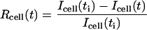(1)

was taken as a measure of the total fraction of bleached fluorophore at time t. The time origin t = 0 s refers here to the time of acquisition of the first postbleach image, which coincided (within 0.01–0.02 s) with the end of the applied bleaching pulse, and t_i corresponds to the time of acquisition of the last prebleach image (i.e., the last image acquired before the bleach), which ranged between t_i = −0.6 s and t_i = −1.9 s. Note that R_cell(t) is an overestimate of the actual fraction of fluorophore bleached in the cell membrane, as only a portion of this membrane can be comprised in the image frame. However, since the total cell intensity is little affected by diffusion in and out of the image frame, and is not affected by diffusion within the image frame, this ratio was a reliable parameter for monitoring the amount of bleach at a given time. For the cells used in our analysis (n = 30), the initial bleached ratio R_cell(0) was in the range 2–8%. After the initial bleach, R_cell(t) usually displayed a slow and near-linear increase with time (and I_cell(t) decreased concomitantly), with total variations after 30 s in the range 0–20%. In some cases, the value of R_cell remained stable (n = 5) or even slightly decreased (n = 4) during the experiment. Such decrease (attributed to noise or to small readjustments of a portion of the cell membrane) never exceeded 4%, and did not affect the recovery in the bleached region. As a rule, we retained in our analysis only experiments for which the variation of I_cell was <5% over the time interval used in the fitting procedure (typically the first 15 s).

Surface and profile bleach configurations

Most isolated OHCs stained with di-8-ANEPPS showed a bright fluorescence localized to the lateral wall, intracellular organelles remaining almost invisible. Two kinds of bleaching experiments were performed on these cells. In one configuration (used by Oghalai et al. (19,37,39)), the focal plane was adjusted vertically at approximately half the diameter of the cell, resulting in a profile view of the OHC membrane as shown in Fig. 1, A and G. The membrane was then bleached on one side of the lateral wall (Fig. 1, H–K). Although this configuration allows good image contrast in the focal plane, the lateral membrane mobility is monitored only in the longitudinal (or axial) direction, and the circular mobility cannot be estimated. In the second configuration, which we refer to as surface bleach, the focal plane was positioned close to the upper surface of the cell membrane (Fig. 1 B). In this configuration, membrane diffusion is monitored in two dimensions (Fig. 1, C–F) and both axial and circular diffusion rates can be measured. To achieve a surface view, the z-position of the microscope's stage was adjusted so that the intensity seen in the center of the cell body would be significant. Due to variability in the experiments, the cell surface settled sometimes slightly above the focal plane (making the lateral boundaries of the cell body to appear brighter due to the curvature of the membrane), and sometimes slightly below (making boundaries less apparent). However, in all experiments, the upper cell surface was well included within the thickness of the optical section (1–2 μm with the objective lens used). This was clear from the fact that the fluorescence in the center of the cell was strongly reduced when the stage was lowered or raised by a few microns. If the surface had been out of focus by more than the thickness of the optical section, almost no fluorescence would have been seen within the bleach spot. It is therefore reasonable to assume that the observed mobility pattern reflected lipid diffusion in the OHC lateral wall, and was little affected by cytoplasmic diffusion or diffusion through the extracellular spaces.

FIGURE 1.

Setup of FRAP experiments on isolated OHCs. (A and B) Confocal sections of the same OHC in profile and surface positions, respectively. The insets show the approximate position of the focal plane with respect to the cell body in each case. Scale bars, 10 μm. (C–F) Detail of the simulation region seen in B, at four times in a FRAP sequence after a surface bleach of the cell (t = 0 s, 1.13 s, 7.9 s, and 24.8 s, where t = 0 s corresponds to the first postbleach image). (G–K) Example of profile bleach experiment, showing the cell just before the bleach (scale bar, 10 μm), and the simulation region at four times after the bleach (t = 0 s, 1.1 s, 2.2 s, and 24 s after the first postbleach image).

Bleach and recovery time issues

When FRAP data are analyzed based on some analytic model of the postbleach fluorescence profile (40,45–48), it is usually assumed that the bleach times are small compared to the time course of recovery, so that one may neglect the effects of diffusion in the membrane during the bleach. As a rule, a bleach period 15 times shorter than the characteristic diffusion time (σ_b being the spatial standard deviation of the bleach intensity spot, and D the diffusion coefficient) is considered short enough for a reliable fit of the recovery curve (40,41). The bleach times in our experiments were variable, ranging from <0.05 s to maximum times of the order of 1 s, whereas half-recovery times ranged between 10 s and 1 min, depending on the cell type, the dye used, and on the bleaching conditions (size, intensity, and duration of the bleach). The half-recovery time τ_1/2 is of the same order, but typically smaller than the characteristic diffusion time (40,41). Our bleach times were thus considered small enough to allow the analysis of fluorescence recovery curves by a theoretical model as described below.

The above bleach time issue does not concern the simulation method described in the next paragraph. In this approach, one simulates the diffusion process starting from the intensity profile observed in the image plane just after the bleach. In contrast with the analytic method of Axelrod et al. (40,41), no assumption is made about the way the bleach was applied (in particular, the fluorescence decay need not be linear), and the shape of the bleach spot can be in principle arbitrary. Therefore, with this method we do not have to care about possible diffusion during the bleach. On the other hand, we must care about the diffusion occurring during scanning after the bleach, since the postbleach images are assumed to represent instantaneous views of the fluorescence profile, at least to a good approximation. The pixel times for the postbleach scanning in our experiments were of 1.44 μs or 2.24 μs depending on the experiment, and the image format was 300 × 400. The corresponding scanning time for one image was ∼0.17 s or 0.27 s (additional line-to-line delays add to much smaller times and may be neglected). The longest image time used was thus >35 times shorter than the typical half-recovery time. Although a small amount of diffusion certainly occurred during the scanning of each image, the corresponding changes in intensity profile were not perceptible and were judged small enough for our purposes.

FRAP experiments during an osmotic challenge

To study the effects of varying membrane tension on lateral diffusion in the OHC membrane, we analyzed a number of FRAP experiments performed while making the medium bath hypotonic to the OHCs. This was achieved by gradually adding 100 μl of distilled water to the solution over a period of ∼20 min. As a result of this osmotic challenge, the cells displayed the morphological changes associated with an increase of turgor pressure, becoming slowly shorter while increasing in radius, and eventually losing their cylindrical shape within a timescale of 10–20 min. The swelling of OHCs in these experiments was a slow process. It took ∼15 min for the cell shown in Fig. 7 to loose its shape. During the time of a single FRAP experiment (∼30 s) neither morphological changes nor the position of the cell's upper surface were perceptible. For each new experiment, the confocal section was readjusted to ensure that the cell surface remained always well in focus during the acquisition.

FIGURE 7.

FRAP experiments on an isolated OHC during osmotic challenge. (A) Plots of the estimated diffusion constants (squares, longitudinal; circles, circumferential) as a function of time during the challenge. (B) Variation of the cell length and radius with time, as observed in the focal plane. (C and D) Plots of the diffusion constants as a function of cell length and cell radius, respectively. (E–H) Confocal views of the OHC used in the experiments at four times during the challenge. Each image shows the cell just after a surface bleach of its membrane, with the simulation rectangle and the estimated diffusion axes, scaled 10 times. Note the gradual change in cell morphology and the visible decrease in axial diffusion rate. Scale bar, 5 μm.

FRAP analysis by two-dimensional simulation

Diffusion model employed

To analyze our FRAP experiments, we followed the approach of Siggia et al. (49), slightly modified to account of a possible anisotropy in the diffusion. The evolution of intensity seen in projection to the focal plane was modeled with the following equation:

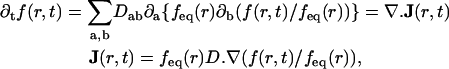(2)

where f(r,t) is the fluorescence intensity at a position r = (x,y) in the focal plane and time t, whereas ∂_t and ∂_a (a = x,y) denote partial derivatives with respect to time and space, respectively. The parameter D = (D_ab) is a 2 × 2 symmetric matrix referred to as the diffusion matrix, which quantifies the mobility of the fluorescent marker in the focal plane. The eigenvectors u₁,u₂ of D define the principal axes of the diffusion process, and the corresponding (positive) eigenvalues D₁, D₂ are the diffusion rates along these axes. The quantity f_eq(r) is the observed steady distribution of intensity in the focal plane, and is included to take account of inhomogeneities (49). To briefly explain the rationale of Eq. 2, the principal assumption made is that the dye molecules in the membrane are in a thermodynamic equilibrium before and after the bleach. The steady distribution is then given by a Boltzmann distribution f_eq(r) = exp(−V(r)) for some effective potential V(r), and Eq. 2 represents the evolution equation (namely, Fokker-Planck equation in the viscous limit) for the distribution of Brownian particles wandering in this potential. Homogeneous diffusion corresponds to a uniform steady state, f_eq being independent of r.

Numerical implementation

The solution to Eq. 2 can be computed by the evolution operator formula

(3)

where P(D,r) denotes the diffusion operator

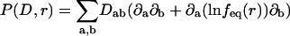(4)

and φ₀(r) stands for the normalized initial density, φ₀(r) = f(r,0)/f_eq(r). Numerical implementation of Eq. 3 was performed in MATLAB (The MathWorks, Natick, MA), using the pixel discretization of the images, while keeping time continuous. With this discretization scheme, the operator exp(tP(D,r)) becomes the exponential of a large sparse matrix, whose action on φ₀(r) can be computed for each observation times in the series. For this we used the Expokit package developed by Sidge (50) (available at http://www.maths.uq.edu.au/expokit), together with custom MATLAB functions implementing Eqs. 2 and 3. The derivative of the solution with respect to D_ab can be computed exactly with the formula

(5)

which is useful for applying a gradient descent algorithm when fitting the simulation to experiments.

Least-squares fit of the model to experiments

For a given FRAP experiment, a simulation region was defined by selecting from the images a small rectangle containing the bleach spot, and Eq. 2 was used to simulate the recovery process inside this rectangle, using the numerical implementation described above.

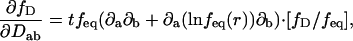
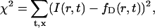
A standard least-squares fit of the simulation to the data was then performed to estimate the diffusion matrix. The fitting procedure consisted in minimizing the following mean-squared error:

(6)

where I(r,t) denotes the image intensity sequence recorded in the focal plane, and f_D(r,t) is the simulated sequence computed for a particular diffusion matrix D. In the above sum, t runs over a range of postbleach acquisition times, and r runs over all pixels in the simulation region. The minimization was performed with respect to the three independent components D_xx, D_yy, D_xy of the diffusion matrix, using the Levenberg-Marquard algorithm. A standard error region in the space of parameters D_ab was estimated as the region in which χ² differs from its minimum value by less than the pixel noise variance σ². This variance was estimated using the formula σ² ≈ χ²/N, valid for N large enough, N being the total number of pixels in the fitted sequence (that is the number of pixels in the simulation region multiplied by the number of acquisition times taken into account in the fit).

A main practical advantage of the above simulation approach is that the bleaching conditions can be arbitrary. The solution to Eq. 2 requires only the knowledge of the equilibrium distribution f_eq(r) and the post-bleach fluorescence profile, both of which are obtained from the data. For each FRAP series, we approximated f_eq(r) by averaging a few (3–5) of the last postbleach images, and by smoothing the result to reduce noise artifacts. The initial state of the simulation was taken to be the first postbleach image. The slow variations in mean fluorescence during the postbleach observations were compensated for by resetting the mean value of the images within the simulation rectangle to that of the first postbleach image. As mentioned above, these variations were small and did not affect intensity values by more than a few percents within the time range over which the simulation was fitted.

Numerical assessment

To check the above least-squares estimation method, we applied it to test image sequences generated by solving Eq. 2 for a known diffusion matrix D and a known initial image. Random Poisson noise was added to these test sequences to mimic the noisy component of confocal images. For sequences having about the same signal/noise ratio as in the experiments, the relative mean-squared error on the elements of D was in the range 1–10%, with an average error <5%. The corresponding error made on the eigenvalues D₁, D₂, relative to their mean value, was in the same range. The estimated angle θ (0 ≤ θ ≤ 45°) determining the orientation of the diffusion axes was accurate within 10°, the error being typically <5°. These error ranges were largely independent of the values of D₁, D₂, θ, and of the initial image used in the simulation.

Analysis of fluorescence recovery curves using line illumination profiles

In a second approach to demonstrate the anisotropy of diffusion in the OHC lateral wall, image intensities were averaged over two Gaussian stripes simulating illumination lines oriented in the axial and the circumferential directions of the cell. The resulting fluorescence recovery curves were then fitted to the theoretical curve derived in the Appendix.

With more details, the analysis of a given experiment proceeded as follows. First, the fractional fluorophore concentration at position r and time t was computed as

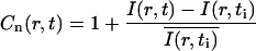(7)

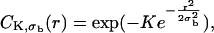
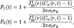
where I(r,t) is the image intensity at pixel position r and time t; I(r,t_i) the image intensity just before the bleach (t = t_i); and denotes the pixel average of I(r,t_i) over the image frame. The above normalization ensures that 0 ≤ C_n(r,t) ≤ 1, subtraction of the prebleach image allowing to compensate for inhomogeneities in membrane staining. Taking t = 0 to be the time of the first postbleach image, C_n(r,0) represents the fractional fluorophore concentration just after the bleach. The intensity profile of the bleach spot being Gaussian in our experiments, the parameters of the bleach were estimated by fitting C_n(r,0) to the function

(8)

assuming a Gaussian bleach spot of spatial standard deviation σ_b, and a linear decay of the fluorophore, with bleach parameter K (cf. Eqs. A2 and A3 of the Appendix.) Usually the fits were very good, allowing reliable estimation of σ_b, with typical values in the range 1–2.5 μm; and of the bleach parameter K, with typical values in the range 1.0–2.0.

Two masks, and , simulating illumination lines passing through the center of the bleach spot, were defined for measuring the diffusion coefficient along the cell's axial and circumferential directions, respectively. was taken constant along the circumferential direction while displaying a Gaussian profile of prescribed standard deviation σ_i along the axial direction (cf. Eq. A4 of the Appendix). As a rule, σ_i was chosen comparable to σ_b. The mask was obtained by a 90° rotation of around the center of the bleach spot. These masks and the bleaching profiles are illustrated in Fig. 4, B and E.

FIGURE 4.

Analysis of fluorescence recovery curves averaged over line-illumination masks. (A and C) Portion of the OHC body surrounding the bleach spot (same cells as in Fig. 2, A and C, respectively). Shadows of the illumination masks and are superimposed (solid lines represent the center axes of the masks, corresponding to the cell's circumferential and axial directions, respectively; dashed lines represent the spatial standard deviation σ_i). (B and D) The intensity profiles of the masks and , together with the fluorescence profile just before and after the bleach, and the corresponding fit to Eq. 8. Estimated parameters of the bleach: σ_b = 2.1 μm, K = 2.9 in case B, and σ_b = 1.3 μm, K = 1.8 in case D. (C and E) Plots of the fractional recovery curves calculated using Eq. 10 (solid curves) and the corresponding fits to Eq. A12 of the Appendix (dashed curves). The insets show the fluorescence intensity profiles around the bleach spot, plotted at different times during the recovery (t = 0s, 2.3 s, 4.5 s, 15.8 s starting from the first postbleach image; solid lines, experimental data; dashed lines, profiles obtained from the two-dimensional simulation).

Assuming full recovery, the quantity C_n(r,t) − 1 corresponds to the fractional depletion of fluorophore at position r and time t, and should be compared to the solution of the diffusion equation satisfying the boundary condition C(∞,t) = 0 (cf. the Appendix). The normalized recovery curves under the illumination lines and were calculated as

(9)

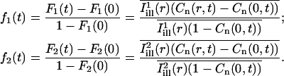
where as before the bars denote pixel averaging and the standard deviations σ_b,σ_i are measured in pixel units. F₁ and F₂ are normalized in this way according to Eq. A12 of the Appendix (keeping in mind that F₀ = C₀ × 2πσ_bσ_i, where C₀ = 1). The experimental curves obtained from Eq. 9 displayed the expected range of values (0.05–0.7). A least-squares fit of F₁ and F₂ based on Eq. A12 was used to obtain estimates of the axial and circumferential diffusion coefficients (D₁ and D₂, respectively), together with the bleach parameter K. This direct fit resulted in values for K consistent with the value obtained by a fit to Eq. 8, and values for D₁, D₂ consistent with the estimates obtained using the two-dimensional simulation approach.

Since the curves defined by Eq. 9 could be sensitive to normalization errors, we performed a second estimation based on the fractional recovery curves (assuming again full recovery of fluorescence):

(10)

Estimates of D₁ and D₂ were then obtained by a least-squares fit based on Eq. A12, using the value of the bleach parameter K obtained using Eq. 8. (The fractional recovery curve being much less sensitive to the value of the bleach parameter, fitting over K would not be suitable in this case.)

RESULTS

Experiments on isolated outer hair cells

Analysis of two-dimensional diffusion in the OHC lateral membrane

Fig. 2 illustrates the results of our analysis of surface bleach experiments. The fluorescence recovery process in the OHC lateral membrane was found to exhibit a distinct orthotropic pattern, with a diffusion rate higher along the cell's axial direction than along its circumferential direction by a factor up to two or more. Fig. 2 A shows the same cell as in Fig. 1 A just after the bleach, together with the principal axes of diffusion estimated from a best fit of the two-dimensional simulation to the data. The quality of the fit is illustrated in Fig. 2 B where two fluorescence curves F_bleach(t) and F_ref(t) are plotted as a function of time: F_bleach(t) was obtained by averaging intensity values within a small mask roughly delimiting the bleach spot. For F_ref(t), we used a reference mask situated near the boundary of the simulation region. Fig. 2, C and D relate to a similar experiment performed on another cell.

FIGURE 2.

Examples of two-dimensional FRAP analysis. (A) View of the same OHC as in Fig. 1 B just after the bleach. The simulation region is highlighted with the principal axes of diffusion. The lengths of the axes are scaled by the corresponding diffusion constants (D₁ = 0.43 ± 0.02 μm²/s, D₂ = 0.18 ± 0.01 μm²/s), with units of length otherwise arbitrary. Scale bar, 5 μm. (B) Intensity curves obtained by averaging the image sequence in two small masks defined in the simulation region (shown as insets). In both graphs, the solid and dashed curves represent the experiment and the fitted simulation, respectively. Note the obvious recovery of intensity within the bleach spot (upper curve), whereas fluorescence loss in photobleaching is observed away from the bleach spot (lower curve). (C) A second example on another cell. Scale bar, 10 μm. The diffusion axes are scaled by the corresponding diffusion constants (D₁ = 0.41 ± 0.03 μm²/s, D₂ = 0.20 ± 0.02 μm²/s), again with arbitrary length units.

The fraction of recovery within the bleach spot was quantified by the ratio R_bleach(t) = (F_bleach(t) − F_bleach(0))/(F_bleach(t_i) − F_bleach(0)), where t_i refers to the time of the last postbleach image and t = 0 is taken to be the time of the first postbleach image (cf. Methods). When computed at the time of last acquisition (t ≈ 30 s), this ratio was of 55% and 78%, in the examples of Fig. 2, A and B, respectively. In most experiments, the fraction of recovery was high, R_bleach being over 60% after 30 s. In fact, the recovery was usually not complete within the duration of the experiments (as can be appreciated in Fig. 2 B), so that R_bleach(t = 30 s) provided only an underestimate of the mobile fraction of fluorophore. Our results thus indicate that the di-8-ANNEPS dye formed a pool of highly mobile molecules in the OHC lateral wall.

For most OHCs, the estimated principal axes of diffusion were well matched with the longitudinal and circumferential axes of the cell. Performing an average over 30 OHCs whose lengths ranged between 25 and 82 μm, we found the values D₁ = 0.36 ± 0.03 μm²/s and D₂ = 0.17 ± 0.02 μm²/s (mean values ± SEs) for the longitudinal and the circumferential diffusion rates, respectively. The corresponding ratio of longitudinal to circumferential diffusion was D₁/D₂ = 2.12 ± 0.43. A negative correlation was observed between the circumferential diffusion rates D₂ and the cell length (correlation coefficient c₂ ≈ −0.7 and p-value of 0.004, derived from Student's distribution). Although significant, this correlation might have reflected differences in the conservation states of long and short cells after isolation, rather than a genuine gradation in membrane fluidity in intact cells. The lack of data concerning variations in OHC membrane tension from the basal to the apical regions of the cochlea (or structural variations of the cortical lattice) makes it difficult to really assess this point. The correlation between the axial diffusion rate and the cell length was not significant (c₁ ≈ −0.09, p-value ≈ 0.74). On the other hand, the spread of both diffusion coefficients over the 30 cells was significant, showing standard deviations of 47% and 59% for D₁ and D₂, respectively, whereas the average measurement errors (estimated from the χ² analysis) were of 12% and 18%.

We further looked for possible variations of the diffusion coefficients along the OHC lateral wall. As is illustrated in Fig. 3 A, we observed no clear correlation between D₁ and D₂ and the position of the bleach spot between the cell's apex and base. Our data rather support the idea of a relative uniformity of the lipid mobility along the main portion of the OHC lateral wall. We stress that this uniformity is to be understood in average, not precluding the presence of local variations in the fluidity of the membrane. Such variations are expected in view of the domain organization of the cortical lattice, and could explain part of the variability seen in our results.

FIGURE 3.

A illustrates the average uniformity of lipid mobility along the OHC lateral wall. The axial and circumferential diffusion coefficients measured on 12 OHCs (circles and squares, respectively) were plotted as a function of the normalized coordinate of the center of the bleach spot along the cell, defined as the ratio x = distance from OHC apex/OHC length. B is the distribution of the axial diffusion angle α_OHC (defined as shown in the inset) measured for 20 OHCs. Superimposed (dashed line) is a distribution obtained by Holley et al. (22) by measuring domain orientations of the cortical lattice in small patches of OHC membrane by electron microscopy. The two distributions (normalized to have the same area) are surprisingly similar with comparable standard deviations (13.9° and 15.4° for α_OHC and domain angle distributions, respectively); their mean values do not differ significantly from 0° (p-value of 0.49 and 0.52, respectively).

We also analyzed the distribution in orientation of the principal diffusion axes in the OHC membrane. We define the axial diffusion angle α_OHC as the angle between the axis of fastest diffusion and the longitudinal axis of the OHC (both axes being oriented toward the cell's apex; see Fig. 3 B). The axial diffusion angle, measured for 25 cells, was not significantly different from zero on average (1.34° ± 2.8°, mean ± SE), but its distribution displayed a significant spread, with a standard deviation of 13.9°. (Single measurement errors were estimated to 6.1°, corresponding to a p-value < 0.01 for reaching the observed standard deviation of 13.9° over 25 samples, according to a χ² test.)

Evidence of diffusion anisotropy from fluorescence recovery curves

The analysis of fluorescence recovery curves averaged over Gaussian illumination lines is illustrated in Fig. 4 for the same two experiments used in Fig. 2. Panels A and D show a portion of the OHC body in each case, with shadows of the two masks and superimposed. The centerlines of the masks (thin solid lines) coincide with the diffusion axes deduced from the two-dimensional simulation, nearly matching the cell's circumferential and axial directions ( and are directed along the slow and the fast axes, respectively). Dashed lines delimit the regions corresponding to a distance of <1 standard deviation σ_i from the centerlines. The intensity profiles of and are reproduced in panels B and E, together with the normalized fluorescence profiles just before and after the bleach, and the corresponding fit to Eq. 8. The fractional fluorescence recovery curves computed with Eq. 10 are plotted in panels C and F (solid curves). Note that the faster diffusion along the axial direction is clear from these curves without any fitting, keeping in mind that the recovery should appear faster or slower when intensity values are averaged along the slow or the fast direction of diffusion, respectively. The fit to Eq. A12 (dashed curves) provided the estimates D₁ = 0.23 μm²/s, D₂ = 0.11 μm²/s for the first cell, and D₁ = 0.42 μm²/s, D₂ = 0.19 μm²/s for the second cell, in reasonable agreement with the values obtained by two-dimensional simulation (D₁ = 0.43 μm²/s, D₂ = 0.18 μm²/s for the first cell; D₁ = 0.41 μm²/s, D₂ = 0.20 μm²/s for the second cell). The use of ad hoc masks simulating illumination lines thus provided a compelling way of demonstrating the anisotropy of lipid diffusion in the OHC lateral wall. However, this approach does not permit a simple and systematic estimation of the orientation of the principal diffusion axes, which has to be guessed or deduced by other means. (One could deduce the fast and slow directions by using a panel of masks oriented at different angles, but this would be rather cumbersome and not very accurate.) Therefore, the two-dimensional simulation approach remained our preferred method of analysis in this study.

Analysis of profile bleach experiments

The apparent diffusion pattern observed in profile bleach experiments with di-8-ANEPPS was highly anisotropic, the diffusion being prominently directed along the cell membrane. This provided confirmation that the marker was concentrated in the OHC lateral wall and did not diffuse significantly in the cytoplasmic or extracellular compartments. In the example shown in Fig. 5, the estimated diffusion rate along the membrane was D_// = 0.24 μm²/s. This coefficient reflected a priori both axial and circumferential diffusion in the cell membrane, which are not separated in the profile bleach configuration. The estimated diffusion rate D_⊥ perpendicular to the membrane was not significantly different from zero (D_⊥ = (0.3 ± 0.4) × 10⁻⁴ μm²/s). This estimate should be considered as reflecting measurement errors, rather than the actual transverse lipid mobility across the OHC membrane (expected to be very small for the dye di-8-ANEPPS). Interestingly, the quality of the fit in the region of the bleach spot was not much affected by changing the value of D_⊥, and performing the same fit under the constraint of isotropic diffusion led to similar lateral diffusion coefficients (0.2 μm²/s in this case). However, the simulation assuming anisotropic diffusion was superior in reproducing the fluorescence loss away from the bleach spot, as can be seen in the lower panel of Fig. 5 B.

FIGURE 5.

(A) Confocal image showing an isolated OHC just after a profile bleach of its membrane. The simulation rectangle is highlighted, together with the estimated diffusion axes. Note the strong anisotropy, directed prominently in the direction of the membrane. Scale bar, 5 μm. (B) Recovery curves averaged within the bleach spot and away from the bleach spot (masks shown in the insets). Solid curves, experiment. Dashed curves, fitted simulation using the anisotropic diffusion model. Dotted curves, fitted simulation assuming isotropic diffusion.

It was clear from our data that the values of the diffusion constants estimated in profile and surface bleaches were similar. In a few experiments (n = 3), the two types of bleaches were applied to the same cell, allowing for a more careful comparison. In these experiments, we found ratios in the range 0.85–1.4 between the profile diffusion constant D_// and the axial diffusion constant D₁ determined from the surface bleach. The ratios between D_// and the circumferential surface diffusion constant D₂ were found in the range 1.15–4.0. We did not attempt to determine the precise relationship between profile and surface diffusion constants. However, the profile values in these experiments appeared to reflect more axial than circumferential diffusion, as one would expect considering the geometry of tangential bleaches.

FRAP experiments on the OHC stereocilia bundle

Although the diffusion rates appeared to be relatively uniform along the OHC lateral wall, higher rates were measured by bleaching the hair bundle of the cell. For OHCs stained with di-8-ANEPPS, we measured values in the range 0.7–1.1 μm²/s for the diffusion constant along stereocilia, with much smaller values in the perpendicular direction, ranging 0.16–0.3 μm²/s. Thus, membrane mobility in the hair bundle was anisotropic and directed along the stereocilia, as might have been expected (Fig. 6). A similar diffusion pattern was observed on the hair bundle for cells stained with the dye RH-795, with the same degree of anisotropy, although smaller diffusion rates (0.47 μm²/s along the stereocilia, and 0.10 μm²/s perpendicular to them, estimated for one cell).

FIGURE 6.

FRAP experiments on the OHC stereocilia bundle. (A) Isolated OHC stained with di-8- ANEPPS. (B) Isolated OHC stained with RH-795. In each case, the first post-bleach image is shown, highlighting the simulation region, and the estimated diffusion axes. Scale bars, 3 μm. (C and D) Details of the simulation rectangle (in each case the last prebleach image was subtracted for a better visualization of the bleach spot) at three times after the bleach. (t = 0 s, 1.4 s, and 16.8 s for C; t = 0 s, 1.1 s, and 13.0 s for D). (E and F) Intensity profiles along lines shown in the insets, at different times during the experiment. (t = 0 s, 1.4 s, 5.6 s, and 19.6 s for E; t = 0 s, 1.1 s, and 9.8 s for F; solid lines, experimental data; dashed lines, two-dimensional simulation; the dotted lines indicate the intensity profiles just before the bleach.)

Effect of an osmotic challenge applied to the cells

Fig. 7 summarizes the results of a series of FRAP experiments performed on the same OHC while the osmolality of the bath solution was decreased from an initial value of 310 mOsm/Kg to a final value of 242 mOsm/Kg. Panels A, C, and D of the figure show the behavior of the axial and circumferential diffusion coefficients as a function of time, cell length, and cell radius, respectively. Panel B is a control plot showing that the OHC had the expected behavior during the challenge, its length gradually decreasing, and its radius gradually increasing. The pattern of membrane diffusion on the cell slowly changed with time, the axial diffusion constant decreasing from 0.32 μm²/s to 0.18 μm²/s from the start to the end of the experiment. The circumferential diffusion appeared only slightly affected by the osmotic challenge, and remained at a value close to 0.17 μm²/s. The decrease in axial diffusion was well correlated with the changes in length and radius of the cell as monitored on the focal plane. In agreement with previous observations (19), the decrease in axial diffusion rate corresponded to a decrease in cell length (and an increase in cell radius), suggesting a direct functional dependency between these parameters.

Experiments with excised temporal bone preparations

Table 1 and Fig. 8 summarize the results of a series of FRAP experiments in several membranes of the intact hearing organ, using three different dyes (di-8-ANEPPS, RH-795, and FM1-43). It was generally not possible to obtain a good match of the focal plane with the membranes' surfaces in situ, and in most experiments a surface configuration could not be used. (However, we performed a limited set of surface FRAP experiments on the membranes of Hensen cells.) As seen above, when applied to a profile bleach, our FRAP analysis provides reliable information on the mobility rate along the membrane profile, but it does not allow one to assess the anisotropy of diffusion in the plane of the membrane. In particular, we could not determine the degree of anisotropy of the membrane diffusion pattern in OHCs, nor in most other cells of the organ. For this reason, the diffusion constants listed in Table 1 refer to profile bleach experiments that were analyzed assuming isotropy of the diffusion process in the image plane. These constants were taken as representative of the mobility rates in the membranes considered. Their typical values for the three dyes used were found in the range 0.1–1 μm²/s, comparable to the values measured on isolated OHCs by Oghalai et al (19,39) and in our study. These values are also in the range found for other cells and generally expected for biological membranes (51). For the two dyes RH-795 and FM1-43, no clear differences were observed in the diffusion values measured in different structures of the organ of Corti; however, the results were characterized by relatively large dispersions. It was also clear that both RH-795 and FM1-43 stained not only the outer plasma membrane of the cells but also intracellular organelles and to some extent the cytoplasm.

TABLE 1.

Effective diffusion rates measured for several cellular membranes of the organ of Corti (mean ± SD for n measurements)

	ANEPPS		RH-795		FM1-43
	D (μm2/s)	% recovery	D (μm2/s)	% recovery	D (μm2/s)	% recovery
OHC	0.30 ± 0.23 (n = 9)	74 ± 9 (n = 9)	0.65 ± 0.35 (n = 27)	75 ± 9 (n = 27)	0.57 ± 0.33 (n = 8)	67 ± 21 (n = 8)
IHC	0.46 ± 0.23 (n = 8)	66 ± 18 (n = 8)	0.72 ± 0.22 (n = 5)	63 ± 7 (n = 5)	0.33 ± 0.09 (n = 5)	63 ± 13 (n = 5)
Pillar cells	0.09 ± 0.004 (n = 2)	53 ± 1 (n = 2)	–	–	0.29 ± 0.003 (n = 2)	81 ± 7 (n = 2)
Hensen cells	0.023 ± 0.01 (n = 5)	13 ± 6 (n = 5)	0.39 ± 0.29 (n = 4)	57 ± 12 (n = 4)	0.84 ± 0.23 (n = 4)	73 ± 11 (n = 4)
Reissner's membrane	0.11 ± 0.06 (n = 2)	48 ± 26 (n = 2)	0.57 ± 0.18 (n = 4)	61 ± 12 (n = 4)	–	–
Nerve fibers	–	–	0.23 ± 0.05 (n = 3)	71 ± 7 (n = 3)	0.18 ± 0.06 (n = 4)	75 ± 14 (n = 4)
Interdental cells	–	–	0.25 ± 0.07 (n = 6)	61 ± 4 (n = 6)	0.19 ± 0.10 (n = 5)	66 ± 8 (n = 5)

Outer hair cells (OHC); inner hair cells (IHC); inner and outer pillar cells; Hensen cells; Reissner's membrane; afferent cochlear fibers below the inner sulcus; interdental cells of the spiral limbus. Empty entries correspond to measurements not performed. Estimated standard deviations represent variability between different cells, which was typically larger than single measurement errors.

FIGURE 8.

Examples of in situ profile bleach experiments with the lipid dye di-8 ANEPPS. (A) Inner hair cells. (B) Outer hair cells. (C) Hensen cells. (D) Outer pillar cells. In each, a focal view of the structure just after the bleach is shown and the corresponding intensity recovering curves averaged within the bleach spot are plotted (solid curves, experiment; dashed curve, simulation). The insets in the images show details of the simulation region at different times in the series (images 1, 2, 3, and last image, starting from the bleach). Note that the recovery in sensory hair cells is faster than in the supporting cells. Scale bars, 5 μm.

In experiments using the dye di-8-ANEPPS, intracellular staining was less significant, although some inner cellular organelles were apparent, as well as a diffuse staining of the cytoplasmic compartments. In comparison, the nuclei of the sensory hair cells were usually little or not stained, and could often be seen as shadows. A clear difference was observed with this dye between the diffusion rates measured in sensory hair cells and in other structures. Lipid mobility in sensory hair cells was found to be ∼3–20 times faster than in supporting cells (Hensen cells and the inner and outer pillars), whereas it was 3–5 times faster than in the Reissner membrane.

Similar remarks could be made concerning the apparent ratios of fluorescence recovery. The percentages of recovery after 30 s measured with the dyes RH-795 and FM-43 were generally above 60%, without clear differences between sensory and supporting cells. By contrast, in preparations stained with di-8-ANEPPS, the percentages of recovery after 30 s were higher in inner and outer hair cells than in the pillar cells, and distinctly higher than in Hensen cells.

Fig. 9 shows two examples of in situ FRAP experiments analyzed in two dimensions. Panel A corresponds to the same experiment as in Fig. 8 A (profile bleach on the membrane of an IHC), whereas panel B corresponds to a surface bleach of a Hensen cell (again stained with di-8-ANEPPS). As in experiments made on isolated OHCs, profile bleach experiments with di-8-ANEPPS resulted in an apparent anisotropic diffusion directed predominantly along the membrane profile. This anisotropy was less strong than observed in profile bleaches of isolated OHCs, and significant diffusion rates perpendicular to the membrane as well as larger error bars on the estimated diffusion axes directions were usually seen. Fig. 9 B shows one of the few surface bleach experiments that we performed on Hensen cells. The pattern of diffusion in this case was nearly isotropic (note the large angular errors in the estimated axes shown in the inset, reflecting the absence of a well-defined direction of diffusion).

FIGURE 9.

Examples of two-dimensional FRAP analysis in situ. (A) Profile bleach on an inner hair cell (same experiment as in Fig. 8 A). (B) Surface bleach on the membrane of a Hensen cell. In each case, the simulation rectangle is highlighted and the estimated diffusion axes are superimposed (scaled by the same factor 3). The inset in panel B shows a magnification of the diffusion axes. Scale bars, 5 μm.

The directions of diffusion axes estimated with the dyes RH-795 and FM1-43 in profile bleach experiments in situ showed more variability than with di-8-ANEPPS, with often no clear relation between the apparent preferred direction of diffusion and the direction of the membrane's profile.

DISCUSSION

Geometric contribution to the anisotropy of lipid mobility in the OHC membrane

Because in a surface bleach configuration the cylindrical OHC membrane is bending away from the focal plane circumferentially, the lateral mobility monitored by FRAP will appear to be anisotropic even if the underlying diffusion in the surface of the membrane is isotropic (52). At a point where the membrane makes an angle θ with the focal plane, the diffusion coefficient is reduced in the circumferential direction by a factor of (cos θ)². This effect would contribute to a faster apparent longitudinal diffusion at positions departing from the cell's center axis, but it cannot fully explain the magnitude of the difference observed in our experiments. Indeed, the bleach was always applied near the upper surface of the OHC, and the half-angle θ spanned by the bleach spot remained relatively small. Typical values of this angle, estimated from the ratio of the radius of the bleach spot to that of the cell, ranged between 10° and 30°, the upper bound being more than conservative. This corresponds to a “geometric” ratio of longitudinal to circumferential diffusion D₁/D₂ in the range 1.05–1.33, whereas the observed average ratio was 2.11 ± 0.42. Another geometric consideration is that lipid diffusion in the OHC plasma membrane could have been affected by the presence of nanoscale axial undulations in this membrane (30,31), which would again result in an orthotropic diffusion pattern (52). However, in this case the higher curvature of the membrane in the axial direction would induce a slower apparent mobility in this direction, opposite to what was observed. We concluded that geometric effects were not responsible for the anisotropy observed in our experiments, although they presumably contributed a small part of it.

Interaction of plasma membrane lipids and membrane skeleton in the OHC

A more plausible assumption is that the anisotropy reflects interactions of membrane lipid molecules tagged by di-8-ANNEPS with structures linked to the underlying cortical lattice. The angular distribution observed for the diffusion axes is of interest in this respect. Although obtained for a relatively small number of cells, this distribution is surprisingly similar to the distribution of domain orientations in the cortical lattice, measured by Holley et al. on small patches of OHC membrane by electron microscopy (22) (Fig. 3 B). A similar angular distribution was also observed in the voltage-induced movements of small microspheres attached to the lateral membrane of living OHCs (53). There is no reason for these distributions to be identical (the domain orientation distribution studied in Holley et al. (22) refer to a single OHC, whereas the distribution measured in Kalinec and Kachar (53) showed a larger spread). However, these similarities suggest that the principal axes of di-8-ANEPPS diffusion in the OHC lateral wall are correlated with the orientation of domains in the cortical lattice. As the sizes of the microdomains in the cortical lattice are estimated in the range 200–1000 nm (22), which is just above the lateral resolution of a confocal microscope (≈500 nm with the objective lens and under the illumination conditions we used), such a correlation would be expected to have observable effects in FRAP experiments. This substantiates the idea that lipid mobility in the OHC reflects the organization of the cell's membrane skeleton.

The OHC is not the only cell in which anisotropy of lateral membrane diffusion appears to be due to interaction with the membrane skeleton. The mobility of succinyl-concanavalin A receptors on the surface of fibroblasts was found long ago to be anisotropic, reflecting presumably interactions of the receptor molecules with the stress fibers of the fibroblasts (54). However, this effect was not too surprising, since succinyl-concanavalin A receptors are rather large proteins that could easily be brought in contact with membrane skeletal proteins. The anisotropy that we observed in the OHC membrane is more surprising, as lipid molecules are too small to span the 25 nm separating the plasma membrane from the orthotropically organized actin and spectrin fibers in the cortical lattice. This possibility should not be dismissed though, for a number of reasons. First, the organization of the OHC lateral wall seen under electron microscopy might be distorted due to the necessary fixation of the sample. In particular, compelling evidence suggests that the cortical lattice is normally compressed longitudinally in a living OHC (55). Such a compressed state should result in an entropic spread of the spectrin filaments out of the plane of the cortical lattice, which could be sufficient for some filaments to reach the plasma membrane. In view of the length of spectrin filaments in the cortical lattice (up to 70–80 nm (22)), a spread of ∼40° would be required (taking into account the fact that the filaments are constrained at both ends). This is large, but since the actual distance to span should be reduced in places, the possibility remains plausible. Specific experiments will be required to measure the actual spread of spectrin in the cortical lattice and test the above idea. In addition, although a lipid molecule taken in isolation might be unlikely to interact directly with the cortical lattice, this does not need to be the case for a small lipid domain containing thousands or more of molecules. In this view, the observed anisotropy could reflect a larger hindrance for lipid diffusion in the direction perpendicular to the spectrin filaments. The possibility of interactions between the OHC plasma membrane and the spectrin component of the cortical lattice is natural, since spectrin-lipid interactions are well-documented in red blood cells and are thought to play a role also in non rhytroid cells (13). Such interactions would influence the lipid organization of the plasma membrane, and could result in a compartmentalization in small domains with different diffusion properties (6). This is in line with the findings of Zhang and Kalinec (56), who reported evidence for a lipid domain organization of the OHC plasma membrane influenced by the cortical lattice, after staining this membrane with the long-chain anionic carbocyanine dye SP-DiIC₁₈(3).

Another possible candidate as a structure affecting lipid diffusion in the OHC membrane is provided by the dense array of particles seen to populate the cytoplasmic side of the OHC plasma membrane under freeze-fracture electron microscopy (33,35,36,53). These particles follow the domain organization of the actin filaments, suggesting that they are linked to the cortical lattice. The presence of a molecular array providing the infrastructure that connects the plasma membrane to the pillars, as suggested by Kalinec and Kachar (53), is also more than plausible. The pillar proteins themselves might well provide the required structures, their insertions in the plasma membrane forming a regular array that could span a nonnegligible portion of the membrane area. Finally, we should mention the membrane protein prestin, present in the OHC plasma membrane and required for the expression of electromotility (57–60). It is not clear to us whether prestin could directly affect the anisotropy of lipid diffusion in the OHC plasma membrane, mainly because the protein is reported to be mobile in this membrane (61). However, all the molecular structures mentioned above could affect the membrane's lipid organization and possibly its phase properties (at least on the cytoplasmic side), thereby influencing indirectly its interaction with the cortical lattice.

Effect of membrane tension on lateral membrane mobility in the OHC

The lateral lipid mobility in our osmotic challenge experiments appeared to be inversely related to membrane tension (and directly related to cell length), in agreement with the previous findings of Oghalai et al. (19,39). One way of interpreting this behavior could be to assume an increasing influence of the cortical lattice caused by its compression as membrane tension increases. If this were the case, our observation that the longitudinal diffusion changed more after the challenge than the circumferential diffusion would be surprising. Indeed, if lipid mobility in the OHC plasma membrane is affected by interaction with spectrin filaments, one could expect that a compression of the cortical lattice would increase this interaction, causing a decrease of the circumferential diffusion coefficient. However, if spectrin filaments are already compressed in the normal state of the cell, it is conceivable that a small additional compression would not have much effect on their interaction with the plasma membrane. A more plausible explanation could be that the observed behavior reflects changes in plasma membrane curvature in response to changes in membrane tension. The increase in axial diffusion rate after cell elongation would then correspond to a flattening of axial membrane undulations, whereas the radial membrane curvature would show little change and circumferential diffusion would be less affected. In support of this view, the observed relationship between axial diffusion rate and cell length (Fig. 7 C) is in qualitative agreement with theoretical predictions based on the model of Saffman and Delbruck (62) for the Brownian motion of cylindrical particles in a fluid membrane, extended to take into account membrane curvature effects (N. S. Gov, Weizmann Institute of Science, personal communication, 2005). Finally, the similar dependencies of the lateral diffusion as a function of membrane tension and transmembrane voltage in the OHC (19) are probably a manifestation of the piezoelectric properties of the cell's lateral wall, now thought to be strongly affected by prestin (63). The observed behavior in an osmotic challenge could therefore involve tension-dependent conformational changes of prestin that would affect the organization of the OHC plasma membrane. Progress in our understanding of the structure of prestin and its relation with the OHC plasma membrane will be needed to really assess this hypothesis.

Lipid mobility in OHC stereocilia

The diffusion pattern in the OHC bundles displayed a high anisotropy directed along the stereocilia. By contrast to the case of the lateral wall, there is a natural explanation for this behavior that does not involve the inner structure of stereocilia. Indeed, individual stereocilia are not resolved by confocal microscopy, so that diffusion in the circumferential direction of their membrane was averaged out in our experiments. As a result, unless significant transport of lipid molecules occurs between adjacent stereocilia, lipid mobility should appear anisotropic (in effect unidimensional) in the hair bundle, a circumstance already pointed out in the context of two-photon FRAP experiments performed in microvilli (64,65). The diffusion anisotropy seen in OHC bundles thus supports small or no exchange of lipid molecules among distinct stereocilia. However, this observation has no implication concerning the interaction of plasma membrane lipids with actin filaments or other components filling the stereocilia. We certainly do not rule out such an interaction, which appears to be required for the gating and adaptation of mechanical transduction channels (66).

The rather large diffusion coefficients measured in OHC stereocilia raise the issue of how lipid transport can occur so fast in the hair bundle without appreciable interstereocilia exchange. The fluorescence recovery curves obtained by averaging intensity values over the bleach spot (data not shown) displayed features characteristic of a diffusion-driven transport; however, a component driven by flow could not be ruled out. Therefore, it is possible that a certain amount of active lipid transport occurs along OHC stereocilia. It will be interesting to investigate this issue further, in view of the highly dynamic mechanisms involved in the regulation of stereocilia length (67).

In situ FRAP experiments

Membrane mobility in membranes of the intact hearing organ

One motivation we had in these experiments was to test the feasibility of FRAP in an intact hearing organ. In this respect, the fact that RH-795 and FM1-43 showed different behaviors than the dye di-8-ANEPPs in situ constitutes a valuable observation that could not have been guessed in advance. Our results also highlight the versatility of the FRAP technique as a method applicable to membranes in an undisrupted biological environment.

An important issue one must consider when doing FRAP in situ is the contribution of bulk (cytoplasmic or extracellular) fluid diffusion to the estimated diffusion coefficient, compared to the actual contribution coming from the two-dimensional mobility in the membrane of interest. Since bulk diffusion is typically orders of magnitude faster than membrane diffusion, even small contributions are likely to add much variability to the results. Bulk diffusion was probably significant for the three dyes tested in our experiments. It could in fact have dominated the mobility observed with the dyes RH-795 and FM1-43. Indeed, besides the significant internalization and higher diffusion rates observed with these dyes in situ as well as in isolated OHCs, the estimated diffusion axes in the profile configuration did generally not correlate with the direction of the membranes. Nevertheless, the diffusion coefficients measured with both dyes were well in the range usually found in living cells. In particular, the diffusion constants estimated were similar in OHCs from the intact hearing organ and in isolated OHCs, despite the obvious differences between the two situations.

The dye di-8-ANEPPs showed a better membrane localization in situ than the two other dyes tested (although this localization was not as specific as in isolated OHCs). The diffusion axes estimated with this dye correlated well with the orientation of the membranes probed. The diffusion constants measured in OHCs from the intact cochlea were also fairly consistent with the estimates obtained on isolated OHCs. This provides us with confidence that the constants measured with this dye reflected the lipid mobility within the selected membranes and were not too much affected by bulk diffusion. The clear differentiation between the sensory and the supporting cells observed with di-8-ANEPPS also supports this conclusion; such a difference would not be expected for a mobility dominated by bulk diffusion, and was indeed not observed with RH-795 and FM1-43.

High lipid mobility in the membranes of sensory hair cells

Our FRAP study in the intact organ of Corti allowed two significant observations to be made. One was that the sensory hair cells showed significantly higher lipid lateral diffusion rates and higher percentages of recovery than did the supporting cells (more precisely the pillar cells and the Hensen cells). The second observation was that lipid diffusion coefficients in IHCs and OHCs where about the same (average values for OHCs being somewhat lower), suggesting that the plasma membranes of both cell types have similar fluid phases in the normal organ. This is interesting in view of the quite different mechanical functions these cells are assumed to have. In the OHC lateral wall, fast lipid mobility is probably correlated with the low concentration of cholesterol present in this membrane (20). As cholesterol is important in determining the bulk phase and mechanical properties of the plasma membrane, it might be that a low level of cholesterol helps the function of prestin and is required for the expression of OHC electromotility (in a similar way, the function of rhodopsin in the rod cell outer segment membranes requires low levels of cholesterol (68)). However, the high fluidity of the plasma membranes of hair cells could be important in other aspects, such as ionic transport across the basolateral membranes of the cells, for example by facilitating the function of K⁺ channels. In this view, our results suggest that the plasma membranes of IHCs might also contain low levels of cholesterol, which would be interesting to check.

The much lower mobility rates in the membranes of supporting cells (especially for Hensen cells) could be a reflection of several factors, including a difference in the lipid phase of these membranes (caused by higher levels of cholesterol and/or differences in membrane protein content), or a stronger hindrance of the motion of lipid molecules by cytoskeletal structures. Although we cannot provide data supporting one possibility or the other, our results underscore the relevance of lateral membrane diffusion as a pertinent functional parameter in the study of cochlear structures in particular, and of living cells in general.

APPENDIX: SERIES SOLUTION FOR THE THEORETICAL FLUORESCENCE RECOVERY CURVE UNDER LINE ILLUMINATION

The quantity of interest in many theoretical approaches to the analysis of FRAP experiments (40,45–48) is the fluorescence recovery curve, defined as a function of time for given bleaching and post-bleach illumination conditions by the formula (omitting factors of no relevance to the following analysis):

(A1)

where C(r,t) denotes the concentration of fluorescent marker at position r and time t, and I_ill(r) denotes the illumination intensity profile. The above integral is taken over the plane where the fluorescence is monitored, in which two-dimensional diffusion is supposed to take place. Following Axelrod et al. (40,41), it is assumed the bleaching pulse is short compared to the characteristic times of transport in the medium of interest, and that fluorescence decay during bleaching is linear. Then the fluorophore concentration just after the bleach has the form

(A2)

where C₀ is the initial concentration of marker (assumed uniform); I_bleach(r) is the intensity profile of the bleach spot, normalized so that I_bleach(0) = 1; K is a constant (the so-called bleach parameter) that determines the strength of the bleach and is proportional to the duration of the pulse and the rate of fluorescence decay in the center of the bleach spot. Under these conditions, the fluorescence curve is a function of the bleach and illumination profiles and of the bleach parameter, F = F_K(t; I_bleach, I_ill). In the cases considered in Axelrod et al. (40) and Meyvis et al. (41), the bleach and illumination profiles are assumed to be identical, I_bleach(r) = I_ill(r). This choice would not be appropriate here, as clearly no diffusion anisotropy can be detected if both I_bleach and I_ill are symmetric. In the context of laser scanning microscopy, it is convenient to use a symmetric bleach spot with an asymmetric illumination profile. Indeed, applying a suitable mask to the images one can readily simulate any illumination profile.

We consider the case where the bleach spot has a two-dimensional (symmetric) Gaussian profile with spatial standard deviation σ_b:

(A3)

whereas the (normalized) illumination profile has the form

(A4)

(x₁,x₂) denoting Cartesian coordinates in the image plane. In other words, the profile corresponds to a Gaussian stripe parallel the Ox₂ axis. The width of the stripe is determined by its transverse standard deviation σ_i.

To derive a theoretical formula for the curve 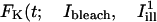), we need to express the fluorophore concentration C(r,t) at a time t after the bleach under the conditions of pure anisotropic diffusion. Let us assume for simplicity that the principal axes of diffusion are directed along Ox₁ and Ox₂. The two-dimensional diffusion matrix is then diagonal,

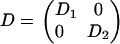(D₁ and D₂ being the diffusion coefficients along Ox₁ and Ox₂, respectively), and C(r,t) obeys the differential equation

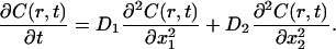(A5)

The solution to this equation for the initial condition given by Eq. A2 is found by Fourier transformation (note that it differs from the isotropic solution only by a rescaling of Ox₁ and Ox₂). To avoid a trivial divergence when averaging C(r,t) over extended masks such as the one defined by Eq. A4, we look for the solution satisfying the boundary condition C(r,t) → 0 for r → ∞. This solution is given by 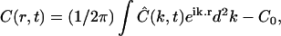where

(A6)

Inserting Eq. A6 into Eq. A1, standard manipulations lead to the general formula

(A7)

where denotes the Fourier transform of the illumination profile.

For the particular profile defined by Eq. A4 we have

(A8)

Inserting now Eqs. A3 and A8 into Eq. A7, one obtains the following:

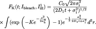(A10)

From this last equation, it is manifest that ) depends on D₁ but not on D₂. More generally, the fluorescence recovery curve obtained for an illumination profile spanning a given line depends only on the diffusion coefficient in the direction perpendicular to this line. The observed recovery is faster when the intensity is averaged along the slow direction, and is conversely slower when averaging along the fast direction.

The series solution we are seeking is obtained from Eq. A10 by expanding the factor 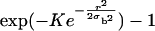in series and integrating term by term, which gives the final result:

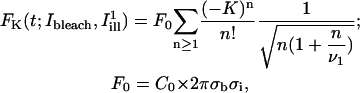(A11)

where , and denotes the characteristic diffusion time along the Ox₁ axis.

Note that with the chosen normalization ) is negative and tends to 0 as t → ∞. For comparison with experimental data, it is convenient to use the rescaled recovery curve

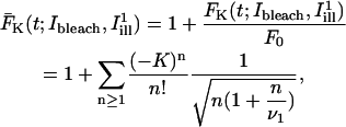(A12)

which obeys the more conventional normalization as t → ∞, and satisfies under most common bleaching conditions.

References

- 1.Edidin, M. 2003. Lipids on the frontier: a century of cell-membrane bilayers. Nat. Rev. Mol. Cell Biol. 4:414–418. [DOI] [PubMed] [Google Scholar]
- 2.Vereb, G., J. Szollosi, J. Matko, P. Nagy, T. Farkas, L. Vigh, L. Matyus, T. A. Waldmann, and S. Damjanovich. 2003. Dynamic, yet structured: The cell membrane three decades after the Singer-Nicolson model. Proc. Natl. Acad. Sci. USA. 100:8053–8058. [DOI] [PMC free article] [PubMed] [Google Scholar]
- 3.Simons, K., and E. Ikonen. 1997. Functional rafts in cell membranes. Nature. 387:569–572. [DOI] [PubMed] [Google Scholar]
- 4.Brown, D. A., and E. London. 1998. Functions of lipid rafts in biological membranes. Annu. Rev. Cell Dev. Biol. 14:111–136. [DOI] [PubMed] [Google Scholar]
- 5.Kusumi, A., and Y. Sako. 1996. Cell surface organization by the membrane skeleton. Curr. Opin. Cell Biol. 8:566–574. [DOI] [PubMed] [Google Scholar]
- 6.Murase, K., T. Fujiwara, Y. Umemura, K. Suzuki, R. Iino, H. Yamashita, M. Saito, H. Murakoshi, K. Ritchie, and A. Kusumi. 2004. Ultrafine membrane compartments for molecular diffusion as revealed by single molecule techniques. Biophys. J. 86:4075–4093. [DOI] [PMC free article] [PubMed] [Google Scholar]
- 7.Dietrich, C., L. A. Bagatolli, Z. N. Volovyk, N. L. Thompson, M. Levi, K. Jacobson, and E. Gratton. 2001. Lipid rafts reconstituted in model membranes. Biophys. J. 80:1417–1428. [DOI] [PMC free article] [PubMed] [Google Scholar]
- 8.Rinia, H. A., M. M. Snel, J. P. van der Eerden, and B. de Kruijff. 2001. Visualizing detergent resistant domains in model membranes with atomic force microscopy. FEBS Lett. 501:92–96. [DOI] [PubMed] [Google Scholar]
- 9.Veatch, S. L., I. V. Polozov, K. Gawrisch, and S. L. Keller. 2004. Liquid domains in vesicles investigated by NMR and fluorescence microscopy. Biophys. J. 86:2910–2922. [DOI] [PMC free article] [PubMed] [Google Scholar]
- 10.Munro, S. 2003. Lipid rafts: elusive or illusive? Cell. 115:377–388. [DOI] [PubMed] [Google Scholar]
- 11.Simons, K., and R. Ehehalt. 2002. Cholesterol, lipid rafts, and disease. J. Clin. Invest. 110:597–603. [DOI] [PMC free article] [PubMed] [Google Scholar]
- 12.Edidin, M. 2003. The state of lipid rafts: from model membranes to cells. Annu. Rev. Biophys. Biomol. Struct. 32:257–283. [DOI] [PubMed] [Google Scholar]
- 13.Sikorski, A. F., B. Hanus-Lorenz, A. Jezierski, and A. R. Dluzewski. 2000. Interaction of membrane skeletal proteins with membrane lipid domain. Acta Biochim. Pol. 47:565–578. [PubMed] [Google Scholar]
- 14.Brownell, W. E., C. R. Bader, D. Bertrand, and Y. de Ribaupierre. 1985. Evoked mechanical responses of isolated cochlear outer hair cells. Science. 227:194–196. [DOI] [PubMed] [Google Scholar]
- 15.Dallos, P. 1992. The active cochlea. J. Neurosci. 12:4575–4585. [DOI] [PMC free article] [PubMed] [Google Scholar]
- 16.Santos-Sacchi, J. 2003. New tunes from Corti's organ: the outer hair cell boogie rules. Curr. Opin. Neurobiol. 13:459–468. [DOI] [PubMed] [Google Scholar]
- 17.Frank, G., W. Hemmert, and A. W. Gummer. 1999. Limiting dynamics of high-frequency electromechanical transduction of outer hair cells. Proc. Natl. Acad. Sci. USA. 96:4420–4425. [DOI] [PMC free article] [PubMed] [Google Scholar]
- 18.He, D. Z., and P. Dallos. 1999. Somatic stiffness of cochlear outer hair cells is voltage-dependent. Proc. Natl. Acad. Sci. USA. 96:8223–8228. [DOI] [PMC free article] [PubMed] [Google Scholar]
- 19.Oghalai, J. S., H. B. Zhao, J. W. Kutz, and W. E. Brownell. 2000. Voltage- and tension-dependent lipid mobility in the outer hair cell plasma membrane. Science. 287:658–661. [DOI] [PMC free article] [PubMed] [Google Scholar]
- 20.Brownell, W. E., A. A. Spector, R. M. Raphael, and A. S. Popel. 2001. Micro- and nanomechanics of the cochlear outer hair cell. Annu. Rev. Biomed. Eng. 3:169–194. [DOI] [PubMed] [Google Scholar]
- 21.Holley, M. C., and J. F. Ashmore. 1988. A cytoskeletal spring in cochlear outer hair cells. Nature. 335:635–637. [DOI] [PubMed] [Google Scholar]
- 22.Holley, M. C., F. Kalinec, and B. Kachar. 1992. Structure of the cortical cytoskeleton in mammalian outer hair cells. J. Cell Sci. 102:569–580. [DOI] [PubMed] [Google Scholar]
- 23.Wada, H., H. Usukura, M. Sugawara, Y. Katori, S. Kakehata, K. Ikeda, and T. Kobayashi. 2003. Relationship between the local stiffness of the outer hair cell along the cell axis and its ultrastructure observed by atomic force microscopy. Hear. Res. 177:61–70. [DOI] [PubMed] [Google Scholar]
- 24.Tolomeo, J. A., and C. R. Steele. 1995. Orthotropic piezoelectric properties of the cochlear outer hair cell wall. J. Acoust. Soc. Am. 97:3006–3011. [DOI] [PubMed] [Google Scholar]
- 25.Spector, A. A., W. E. Brownell, and A. S. Popel. 1998. Estimation of elastic moduli and bending stiffness of the anisotropic outer hair cell wall. J. Acoust. Soc. Am. 103:1007–1011. [DOI] [PubMed] [Google Scholar]
- 26.Spector, A. A., W. E. Brownell, and A. S. Popel. 1998. Elastic properties of the composite outer hair cell wall. Ann. Biomed. Eng. 26:157–165. [DOI] [PubMed] [Google Scholar]
- 27.Sugawara, M., and H. Wada. 2001. Analysis of elastic properties of outer hair cell wall using shell theory(1). Hear. Res. 160:63–72. [DOI] [PubMed] [Google Scholar]
- 28.Zelenskaya, A., J. B. de Monvel, D. Pesen, M. Radmacher, J. H. Hoh, and M. Ulfendahl. 2005. Evidence for a highly elastic shell-core organization of cochlear outer hair cells by local membrane indentation. Biophys. J. 88:2982–2993. [DOI] [PMC free article] [PubMed] [Google Scholar]
- 29.Spector, A. A., M. Ameen, P. G. Charalambides, and A. S. Popel. 2002. Nanostructure, effective properties, and deformation pattern of the cochlear outer hair cell cytoskeleton. J. Biomech. Eng. 124:180–187. [DOI] [PubMed] [Google Scholar]
- 30.Smith, C. A. 1968. Ultrastructure of the organ of Corti. Adv. Sci. 24:419–433. [PubMed] [Google Scholar]
- 31.Ulfendahl, M., and N. Slepecky. 1988. Ultrastructural correlates of inner ear sensory cell shortening. J. Submicrosc. Cytol. Pathol. 20:47–51. [PubMed] [Google Scholar]
- 32.Flock, A., B. Flock, and M. Ulfendahl. 1986. Mechanisms of movement in outer hair cells and a possible structural basis. Arch. Otorhinolaryngol. 243:83–90. [DOI] [PubMed] [Google Scholar]
- 33.Gulley, R. L., and T. S. Reese. 1977. Regional specialization of the hair cell plasmalemma in the organ of Corti. Anat. Rec. 189:109–123. [DOI] [PubMed] [Google Scholar]
- 34.Saito, K. 1983. Fine structure of the sensory epithelium of guinea-pig organ of Corti: subsurface cisternae and lamellar bodies in the outer hair cells. Cell Tissue Res. 229:467–481. [DOI] [PubMed] [Google Scholar]
- 35.Forge, A. 1991. Structural features of the lateral walls in mammalian cochlear outer hair cells. Cell Tissue Res. 265:473–483. [DOI] [PubMed] [Google Scholar]
- 36.Kalinec, F., M. C. Holley, K. H. Iwasa, D. J. Lim, and B. Kachar. 1992. A membrane-based force generation mechanism in auditory sensory cells. Proc. Natl. Acad. Sci. USA. 89:8671–8675. [DOI] [PMC free article] [PubMed] [Google Scholar]
- 37.Oghalai, J. S., A. A. Patel, T. Nakagawa, and W. E. Brownell. 1998. Fluorescence-imaged microdeformation of the outer hair cell lateral wall. J. Neurosci. 18:48–58. [DOI] [PMC free article] [PubMed] [Google Scholar]
- 38.Morimoto, N., R. M. Raphael, A. Nygren, and W. E. Brownell. 2002. Excess plasma membrane and effects of ionic amphipaths on mechanics of outer hair cell lateral wall. Am. J. Physiol. Cell Physiol. 282:C1076–C1086. [DOI] [PubMed] [Google Scholar]
- 39.Oghalai, J. S., T. D. Tran, R. M. Raphael, T. Nakagawa, and W. E. Brownell. 1999. Transverse and lateral mobility in outer hair cell lateral wall membranes. Hear. Res. 135:19–28. [DOI] [PubMed] [Google Scholar]
- 40.Axelrod, D., D. E. Koppel, J. Schlessinger, E. Elson, and W. W. Webb. 1976. Mobility measurement by analysis of fluorescence photobleaching recovery kinetics. Biophys. J. 16:1055–1069. [DOI] [PMC free article] [PubMed] [Google Scholar]
- 41.Meyvis, T. K., S. C. De Smedt, P. Van Oostveldt, and J. Demeester. 1999. Fluorescence recovery after photobleaching: a versatile tool for mobility and interaction measurements in pharmaceutical research. Pharm. Res. 16:1153–1162. [DOI] [PubMed] [Google Scholar]
- 42.Flock, A., E. Scarfone, and M. Ulfendahl. 1998. Vital staining of the hearing organ: visualization of cellular structure with confocal microscopy. Neuroscience. 83:215–228. [DOI] [PubMed] [Google Scholar]
- 43.Shehata, W. E., W. E. Brownell, and R. Dieler. 1991. Effects of salicylate on shape, electromotility and membrane characteristics of isolated outer hair cells from guinea pig cochlea. Acta Otolaryngol. 111:707–718. [DOI] [PubMed] [Google Scholar]
- 44.Ulfendahl, M., A. Flock, and S. M. Khanna. 1989. A temporal bone preparation for the study of cochlear micromechanics at the cellular level. Hear. Res. 40:55–64. [DOI] [PubMed] [Google Scholar]
- 45.Soumpasis, D. M. 1983. Theoretical analysis of fluorescence photobleaching recovery experiments. Biophys. J. 41:95–97. [DOI] [PMC free article] [PubMed] [Google Scholar]
- 46.Kubitscheck, U., P. Wedekind, and R. Peters. 1994. Lateral diffusion measurement at high spatial resolution by scanning microphotolysis in a confocal microscope. Biophys. J. 67:948–956. [DOI] [PMC free article] [PubMed] [Google Scholar]
- 47.Gordon, G. W., B. Chazotte, X. F. Wang, and B. Herman. 1995. Analysis of simulated and experimental fluorescence recovery after photobleaching. Data for two diffusing components. Biophys. J. 68:766–778. [DOI] [PMC free article] [PubMed] [Google Scholar]
- 48.Braeckmans, K., L. Peeters, N. N. Sanders, S. C. De Smedt, and J. Demeester. 2003. Three-dimensional fluorescence recovery after photobleaching with the confocal scanning laser microscope. Biophys. J. 85:2240–2252. [DOI] [PMC free article] [PubMed] [Google Scholar]
- 49.Siggia, E. D., J. Lippincott-Schwartz, and S. Bekiranov. 2000. Diffusion in inhomogeneous media: theory and simulations applied to whole cell photobleach recovery. Biophys. J. 79:1761–1770. [DOI] [PMC free article] [PubMed] [Google Scholar]
- 50.Sidge, R. B. 1998. EXPOKIT: A software package for computing matrix exponentials. ACM Trans. Math. Soft. 24:130–156. [Google Scholar]
- 51.Almeida, P. F. F., and W. L. Vaz. 1995. Lateral diffusion in membranes. In Handbook of Biological Physics. R. Lipowsky and E. Sackmann, editors. Elsevier Science B.V., Amsterdam, The Netherlands. 305–357.
- 52.Aizenbud, B. M., and N. D. Gershon. 1985. Diffusion of molecules on biological membranes of nonplanar form. II. Diffusion anisotropy. Biophys. J. 48:543–546. [DOI] [PMC free article] [PubMed] [Google Scholar]
- 53.Kalinec, F., and B. Kachar. 1995. Structure of the Electromechanical Transduction Mechanism in Mammalian Outer Hair Cells. In Active Hearing, 1st ed. A. Flock, D. Ottoson, and M. Ulfendahl, editors. Pergamon, Burlington, MA. 181–193.
- 54.Smith, B. A., W. R. Clark, and H. M. McConnell. 1979. Anisotropic molecular motion on cell surfaces. Proc. Natl. Acad. Sci. USA. 76:5641–5644. [DOI] [PMC free article] [PubMed] [Google Scholar]
- 55.Chan, E., A. Suneson, and M. Ulfendahl. 1998. Acoustic trauma causes reversible stiffness changes in auditory sensory cells. Neuroscience. 83:961–968. [DOI] [PubMed] [Google Scholar]
- 56.Zhang, M., and F. Kalinec. 2002. Structural microdomains in the lateral plasma membrane of cochlear outer hair cells. J. Assoc. Res. Otolaryngol. 3:289–301. [DOI] [PMC free article] [PubMed] [Google Scholar]
- 57.Zheng, J., W. Shen, D. Z. He, K. B. Long, L. D. Madison, and P. Dallos. 2000. Prestin is the motor protein of cochlear outer hair cells. Nature. 405:149–155. [DOI] [PubMed] [Google Scholar]
- 58.Belyantseva, I. A., H. J. Adler, R. Curi, G. I. Frolenkov, and B. Kachar. 2000. Expression and localization of prestin and the sugar transporter GLUT-5 during development of electromotility in cochlear outer hair cells. J. Neurosci. 20:1–5. [DOI] [PMC free article] [PubMed]
- 59.Oliver, D., D. Z. He, N. Klocker, J. Ludwig, U. Schulte, S. Waldegger, J. P. Ruppersberg, P. Dallos, and B. Fakler. 2001. Intracellular anions as the voltage sensor of prestin, the outer hair cell motor protein. Science. 292:2340–2343. [DOI] [PubMed] [Google Scholar]
- 60.Liberman, M. C., J. Gao, D. Z. He, X. Wu, S. Jia, and J. Zuo. 2002. Prestin is required for electromotility of the outer hair cell and for the cochlear amplifier. Nature. 419:300–304. [DOI] [PubMed] [Google Scholar]
- 61.Santos-Sacchi, J., and H. B. Zhao. 2003. Excitation of fluorescent dyes inactivates the outer hair cell integral membrane motor protein prestin and betrays its lateral mobility. Pflugers Arch. 446:617–622. [DOI] [PubMed] [Google Scholar]
- 62.Saffman, P. G., and M. Delbruck. 1975. Brownian motion in biological membranes. Proc. Natl. Acad. Sci. USA. 72:3111–3113. [DOI] [PMC free article] [PubMed] [Google Scholar]
- 63.Brownell, W. E. 2005. The piezoelectric outer hair cell. In Vertebrate Hair Cells. Springer Handbook of Auditory Research. A. N. Popper, R. R. R. Fay, and A. Eatock, editors.
- 64.Coscoy, S., F. Waharte, A. Gautreau, M. Martin, D. Louvard, P. Mangeat, M. Arpin, and F. Amblard. 2002. Molecular analysis of microscopic ezrin dynamics by two-photon FRAP. Proc. Natl. Acad. Sci. USA. 99:12813–12818. [DOI] [PMC free article] [PubMed] [Google Scholar]
- 65.Waharte, F., C. M. Brown, S. Coscoy, E. Coudrier, and F. Amblard. 2005. A two-photon FRAP analysis of the cytoskeleton dynamics in the microvilli of intestinal cells. Biophys. J. 88:1467–1478. [DOI] [PMC free article] [PubMed] [Google Scholar]
- 66.Hirono, M., C. S. Denis, G. P. Richardson, and P. G. Gillespie. 2004. Hair cells require phosphatidylinositol 4,5-bisphosphate for mechanical transduction and adaptation. Neuron. 44:309–320. [DOI] [PubMed] [Google Scholar]
- 67.Lin, H. W., M. E. Schneider, and B. Kachar. 2005. When size matters: the dynamic regulation of stereocilia lengths. Curr. Opin. Cell Biol. 17:55–61. [DOI] [PubMed] [Google Scholar]
- 68.Albert, A. D., and K. Boesze-Battaglia. 2005. The role of cholesterol in rod outer segment membranes. Prog. Lipid Res. 44:99–124. [DOI] [PMC free article] [PubMed] [Google Scholar]