Abstract
Background
Supervised classification is fundamental in bioinformatics. Machine learning models, such as neural networks, have been applied to discover genes and expression patterns. This process is achieved by implementing training and test phases. In the training phase, a set of cases and their respective labels are used to build a classifier. During testing, the classifier is used to predict new cases. One approach to assessing its predictive quality is to estimate its accuracy during the test phase. Key limitations appear when dealing with small-data samples. This paper investigates the effect of data sampling techniques on the assessment of neural network classifiers.
Results
Three data sampling techniques were studied: Cross-validation, leave-one-out, and bootstrap. These methods are designed to reduce the bias and variance of small-sample estimations. Two prediction problems based on small-sample sets were considered: Classification of microarray data originating from a leukemia study and from small, round blue-cell tumours. A third problem, the prediction of splice-junctions, was analysed to perform comparisons. Different accuracy estimations were produced for each problem. The variations are accentuated in the small-data samples. The quality of the estimates depends on the number of train-test experiments and the amount of data used for training the networks.
Conclusion
The predictive quality assessment of biomolecular data classifiers depends on the data size, sampling techniques and the number of train-test experiments. Conservative and optimistic accuracy estimations can be obtained by applying different methods. Guidelines are suggested to select a sampling technique according to the complexity of the prediction problem under consideration.
Background
Supervised classification plays a key role in bioinformatics. One such application is the recognition of expression patterns for disease classification and gene function discovery [1,2]. It requires the construction of a model, which processes input vectors representing cases, and predicts the class or category associated to the cases under consideration. A class may represent, for example, a type of cancer or a biological function [3,4]. This recognition process is achieved by implementing training and test phases. In the training phase, also known as the learning phase, a set of cases and their respective labels are used to build a classification model. In the test or validation phase, the trained classifier is used to predict new cases. Artificial neural networks (ANNs), such as the back-propagation feed-forward neural network (BP-ANN) [5] have become useful tools to perform classification applications in functional genomics, [6]. An ANN may be trained, for instance, to differentiate genes or experiments by adapting mathematical structures known as weights. This process aims to optimise the prediction of classes for each case in the training set. Generalisation is the ability to correctly classify cases unseen during training. ANNs have been successful in a number of diagnostic, prognostic and systems biology applications [2,7]. The reader is referred to [7] for a review on neural networks and their applications in functional genomics.
One basic approach to assessing the predictive quality of a classifier is to estimate its accuracy during the test phase. Ideally an ANN classifier will be able to generalise if: a) its architecture and learning parameters have been properly defined, and b) enough training data are available. Nevertheless, the second condition is difficult to achieve due to resource and time constraints. Key limitations appear when dealing with small-data samples, which is a common feature observed in many microarray studies [7,8]. With a small training dataset, an ANN may not be able to accurately represent the data under analysis. Similarly, a small test dataset may contribute to an inaccurate performance assessment. Moreover, this accuracy estimation task may have a strong impact on the selection of features for knowledge discovery applications [8].
These factors are relevant for expression data classification and other genomic studies because: a) the biological problems under analysis are complex, and b) the available data are limited, incomplete and inaccurate. Solutions have been proposed to address the processing of incomplete and inaccurate data [7]. Small sample issues and the estimation of the prediction accuracy of classifiers have received relatively little attention [2,8]. Scientists have traditionally dealt with the problem of limited data by carefully selecting relevant cases for training and testing [8]. However, the complexity of most classification tasks and the underlying biological problems require the implementation of automated, effective and efficient solutions to reduce the bias and variance contributions from small datasets.
There are three techniques to estimate the prediction accuracy of classifiers such as ANNs: a) cross-validation, b) leave-one-out, and c) bootstrap. They comprise different methods for splitting or sampling the data. These techniques have demonstrated the reduction of either the estimation bias or the variance introduced by a small dataset [9].
The cross-validation method [10] randomly divides the data into the training and test sets. This process is repeated several times and the classification performance is the average of the individual test estimates. However, the classifier may not be able to accurately predict new cases if the amount of data used for training is too small. At the same time, the quality assessment may not be accurate if the portion of data used for testing is too small. This sampling technique has been studied in regression and classification tasks for engineering and medical informatics applications [11,12]. Some investigations have suggested a split between 25%–50% of the available data as an optimal partition for testing [9].
The Leave-one-out method represents a special case of the cross-validation technique [11]. Given n cases available in a dataset, a classifier is trained on (n-1) cases, and then is tested on the case that was left out. This process is repeated n times until every case in the dataset has been included once as a cross-validation instance. The results are averaged across the n test cases to estimate the classifier's prediction performance.
In the bootstrap method a training dataset is generated by sampling with replacement n times from the available n cases [13]. The classifier is trained on this set and then tested on the original dataset. This process is repeated several times, and the classifier's accuracy estimate is the average of these individual estimates.
This paper investigates the effect of data sampling techniques on the performance assessment of BP-ANN classifiers for biomolecular data. Two small-sample datasets were analysed: Microarray data originating from a study on leukaemia, and microarray data originating from small, round blue-cell tumours (SRBCT). A larger dataset consisting of splice-junctions gene sequences was analysed to perform comparisons.
The main research goals of this study are: a) to establish differences between data sampling techniques when applied to small and larger datasets, b) to study the response of these methods to the size and number of train-test sets, and c) to investigate criteria for the selection of sampling techniques.
Results
The prediction accuracy of each classification model was assessed by applying the sampling techniques and monitoring its response to several thousands train-test experiments. The classification accuracy of an individual experiment is defined as the proportion of correctly classified cases of all cases available. Several thousand BP-ANNs were trained and tested on the datasets described above.
Classification of expression patterns in a leukaemia study
The data consisted of 72 cases categorised into two classes: Acute myeloid leukemia (AML) and acute lymphoblastic leukemia (ALL), which are represented by the expression values of 50 genes with suspected roles in processes relevant to these diseases. These classes included 25 and 47 cases respectively. The original datasets, experimental protocols and further analyses can be found in [14] and at the MIT Whitehead Institute Web site http://www.genome.wi.mit.edu/MPR. All of the networks were trained and tested using the same learning parameters. The BP-ANN architectures comprised 50 input nodes, 5 hidden nodes and 2 output nodes. Each output node encodes one of the leukaemia classes.
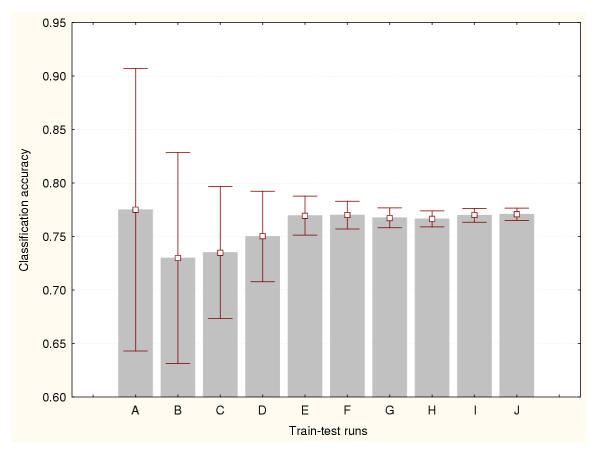
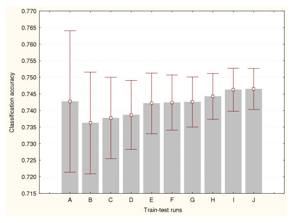
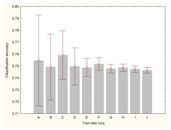
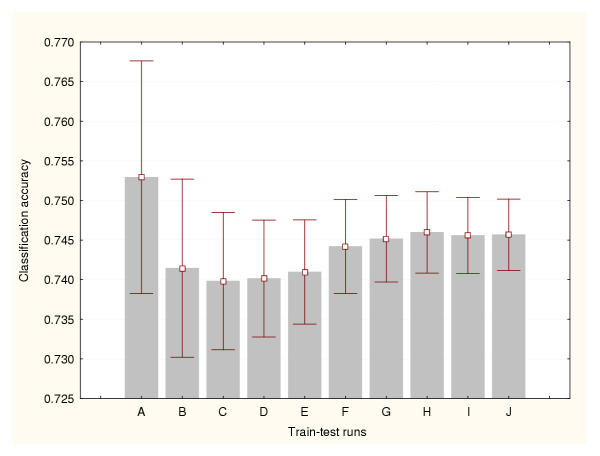
In this study, the cross-validation results were analysed for three different data splitting methods: a) 50% of the available cases were used for training the classifiers and the remaining 50% for testing, b) 75% for training and 25% for testing, and c) 95% for training and 5% for testing. Figures 1, 2 and 3 show the prediction accuracy values and their confidence intervals (95% confidence) obtained for each splitting technique respectively. Figure 1 indicates that more than 500 train-test runs are required to significantly reduce the variance of these estimates (confidence interval size for the mean equal to 0.01). The smallest numbers of train-test experiments allow the generation of the highest or most optimistic accuracy estimates. This method produced the lowest (most conservative) cross-validation accuracy estimates. Figure 2 shows that more than 1000 train-test runs are required to significantly reduce the variance of this cross-validation estimate. Again, the smallest numbers of train-test experiments generated the most optimistic accuracy estimates. The 95%–5% cross-validation method (Figure 3) requires more than 5000 train-test runs to reduce the variance of these estimates. This method produced the most optimistic cross-validation accuracy estimates. The leave-one-out method estimated the highest prediction accuracy for this classification problem (0.81). The results generated by the bootstrap method are depicted in Figure 4. It indicates that more than 1000 train-test runs were required to achieve a confidence interval size equal to 0.01. The bootstrap result originating from 1000 train-test runs is not significantly different than that produced by the 50%–50% cross-validation technique based on 1000 train-test runs. These results suggest that the estimation of high accuracy values may be associated with an increase of the size of the training datasets.
Figure 1.
Accuracy estimation for leukaemia data classifier (I) Cross-validation method based on a 50%–50% splitting. Prediction accuracy values and the confidence intervals for the means (95% confidence) are depicted for a number of train-test runs. A: 10 train-test runs, B: 25 train-test runs, C: 50 train-test runs, D: 100 train-test runs, E: 500 train-test runs, F: 1000 train-test runs, G: 2000 train-test runs, H: 3000 train-test runs, I: 4000 train-test runs, J: 5000 train-test runs.
Figure 2.
Accuracy estimation for leukaemia data classifier (II) Cross-validation method based on a 75%–25% splitting. Prediction accuracy values and the confidence intervals for the means (95% confidence) are depicted for a number of train-test runs. A: 10 train-test runs, B: 25 train-test runs, C: 50 train-test runs, D: 100 train-test runs, E: 500 train-test runs, F: 1000 train-test runs, G: 2000 train-test runs, H: 3000 train-test runs, I: 4000 train-test runs, J: 5000 train-test runs.
Figure 3.
Accuracy estimation for leukaemia data classifier (III) Cross-validation method based on a 95%–5% splitting. Prediction accuracy values and the confidence intervals for the means (95% confidence) are depicted for a number of train-test runs. A: 10 train-test runs, B: 25 train-test runs, C: 50 train-test runs, D: 100 train-test runs, E: 500 train-test runs, F: 1000 train-test runs, G: 2000 train-test runs, H: 3000 train-test runs, I: 4000 train-test runs, J: 5000 train-test runs.
Figure 4.
Accuracy estimation for leukaemia data classifier (IV) Bootstrap method. Prediction accuracy values and the confidence intervals for the means (95% confidence) are depicted for a number of train-test runs. A: 100 train-test runs, B: 200 train-test runs, C: 300 train-test runs, D: 400 train-test runs, E: 500 train-test runs, F: 600 train-test runs, G: 700 train-test runs, H: 800 train-test runs, I: 900 train-test runs, J: 1000 train-test runs.
Classification of expression patterns in SRBCT
The data consisted of 88 cases categorised into four classes: Ewing family of tumors (EWS), rhabdomyosarcoma (RMS), Burkitt lymphomas (BL) and neuroblastomas (NB), which were represented by the expression values of 2308 genes with suspected roles in processes relevant to these tumors. Classes EWS, BL, NB and RMS contained 30, 11, 19 and 28 cases respectively. Principal component analysis was applied to reduce the dimensionality of the cases. As indicated in [6], the 10 dominant components per case were used to train the networks. The original datasets, experimental protocols and further analyses can be found in [6]. All of the networks were trained and tested using the same learning parameters. The BP-ANN architectures comprised 10 input nodes, 8 hidden nodes and 4 output nodes. Each output node encodes one of the tumor classes.
Figures 5, 6 and 7 illustrate the prediction accuracy mean values and their confidence intervals (95% confidence) obtained for each cross-validation technique respectively. Figure 5 indicates that more than 500 train-test runs are required to achieve a confidence interval size equal to 0.01 for this splitting method. The smallest numbers of train-test experiments allow the generation of the most optimistic accuracy estimates. However, in general this method produced the most conservative cross-validation accuracy estimates. Figure 6 shows that more than 1000 train-test runs are required to significantly reduce the variance of this cross-validation estimate. The 95%–5% cross-validation method (Figure 7) requires more than 5000 train-test runs to achieve the same. This method produced the most optimistic cross-validation accuracy estimates. The leave-one-out method produced the highest accuracy estimate for this dataset (0.79). Figure 8 illustrates the results generated by the bootstrap method. In this situation more than 900 train-test runs were required to achieve a confidence interval size equal to 0.01. These results also suggest that the estimation of high accuracy values may be linked to an increase of the size of the training datasets.
Figure 5.
Accuracy estimation for the SRBCT classifier (I) Cross-validation method based on a 50%–50% splitting. Prediction accuracy values and the confidence intervals for the means (95% confidence) are depicted for a number of train-test runs. A: 10 train-test runs, B: 25 train-test runs, C: 50 train-test runs, D: 100 train-test runs, E: 500 train-test runs, F: 1000 train-test runs, G: 2000 train-test runs, H: 3000 train-test runs, I: 4000 train-test runs, J: 5000 train-test runs.
Figure 6.
Accuracy estimation for the SRBCT classifier (II) Cross-validation method based on a 75%–25% splitting. Prediction accuracy values and the confidence intervals for the means (95% confidence) are depicted for a number of train-test runs. A: 10 train-test runs, B: 25 train-test runs, C: 50 train-test runs, D: 100 train-test runs, E: 500 train-test runs, F: 1000 train-test runs, G: 2000 train-test runs, H: 3000 train-test runs, I: 4000 train-test runs, J: 5000 train-test runs.
Figure 7.
Accuracy estimation for the SRBCT classifier (III) Cross-validation method based on a 95%–5% splitting. Prediction accuracy values and the confidence intervals for the means (95% confidence) are depicted for a number of train-test runs. A: 10 train-test runs, B: 25 train-test runs, C: 50 train-test runs, D: 100 train-test runs, E: 500 train-test runs, F: 1000 train-test runs, G: 2000 train-test runs, H: 3000 train-test runs, I: 4000 train-test runs, J: 5000 train-test runs.
Figure 8.
Accuracy estimation for the SRBCT classifier (IV) Bootstrap method. Prediction accuracy values and the confidence intervals for the means (95% confidence) are depicted for a number of train-test runs. A: 100 train-test runs, B: 200 train-test runs, C: 300 train-test runs, D: 400 train-test runs, E: 500 train-test runs, F: 600 train-test runs, G: 700 train-test runs, H: 800 train-test runs, I: 900 train-test runs, J: 1000 train-test runs.
Classification of splice-junction sequences
This dataset consisted of 2000 cases divided into three categories: Exon/intron boundaries (EI), intron/exon boundaries (IE) and neither (N). Each class comprised 464, 485 and 1051 cases respectively. Each case is represented by 60 features, which encode the nucleotide composition of each sequence.
The original datasets and further information can be obtained at: http://www.liacc.up.pt/ML/statlog/datasets/dna/dna.doc.html.
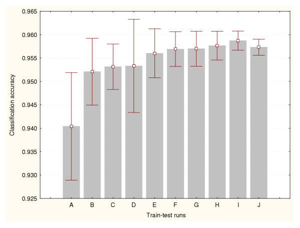
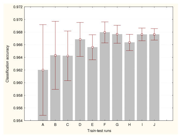
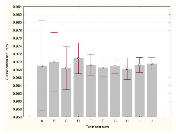
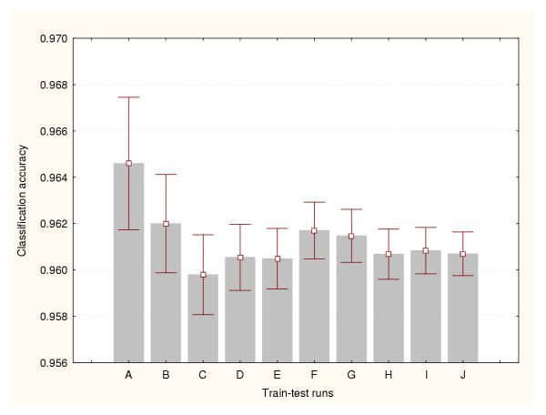
Each BP-ANN consisted of 60 input nodes, 10 hidden nodes and 3 output nodes. The sampling techniques generated different accuracy estimates. But unlike the expression datasets, there were relatively less significant differences between methods. There are not significant statistical differences between the estimates produced by the train-test experiments belonging to a particular data sampling method. Moreover, less train-test runs are required to reduce the variance of the cross-validation and bootstraps estimates. Figures 9, 10 and 11 portray the mean accuracy estimates and their confidence intervals (95% confidence) obtained for each cross-validation technique respectively. Figure 9 indicates that more than 300 train-test runs are required to significantly reduce the variance of the 50%–50% cross-validation estimates. However, a confidence interval size equal to 0.01 had been achieved earlier for only 50 runs. In general this method produced the most conservative cross-validation accuracy estimates. Figure 10 shows that only 50 train-test runs are required to significantly reduce the variance of the 75%–25% cross-validation estimates. The 95%–5% cross-validation method (Figure 11) needed only 100 train-test runs to achieve the same. This splitting method generated one of the most optimistic accuracy estimates for this dataset. The leave-one-out method also produced one of highest accuracy estimates for this problem (0.97). There are not significant differences between the accuracy estimates produced by these two methods. Finally, Figure 12 illustrates the results generated by the bootstrap technique. In this method only 100 train-test runs were required to significantly reduce the variance of the estimates.
Figure 9.
Accuracy estimation for the splice-junction sequence classifier (I) Cross-validation method based on a 50%–50% splitting. Prediction accuracy values and the confidence intervals for the means (95% confidence) are depicted for a number of train-test runs. A: 10 train-test runs, B: 25 train-test runs, C: 50 train-test runs, D: 100 train-test runs, E: 200 train-test runs, F: 300 train-test runs, G: 400 train-test runs, H: 500 train-test runs, I: 800 train-test runs, J: 1000 train-test runs.
Figure 10.
Accuracy estimation for the splice-junction sequence classifier (II) Cross-validation method based on a 75%–25% splitting. Prediction accuracy values and the confidence intervals for the means (95% confidence) are depicted for a number of train-test runs. A: 10 train-test runs, B: 25 train-test runs, C: 50 train-test runs, D: 100 train-test runs, E: 200 train-test runs, F: 300 train-test runs, G: 400 train-test runs, H: 500 train-test runs, I: 800 train-test runs, J: 1000 train-test runs.
Figure 11.
Accuracy estimation for the splice-junction sequence classifier (III) Cross-validation method based on a 95%–5% splitting. Prediction accuracy values and the confidence intervals for the means (95% confidence) are depicted for a number of train-test runs. A: 10 train-test runs, B: 25 train-test runs, C: 50 train-test runs, D: 100 train-test runs, E: 200 train-test runs, F: 300 train-test runs, G: 400 train-test runs, H: 500 train-test runs, I: 800 train-test runs, J: 1000 train-test runs.
Figure 12.
Accuracy estimation for the splice-junction sequence classifier (IV) Bootstrap method. Prediction accuracy values and the confidence intervals for the means (95% confidence) are depicted for a number of train-test runs. A: 100 train-test runs, B: 200 train-test runs, C: 300 train-test runs, D: 400 train-test runs, E: 500 train-test runs, F: 600 train-test runs, G: 700 train-test runs, H: 800 train-test runs, I: 900 train-test runs, J: 1000 train-test runs.
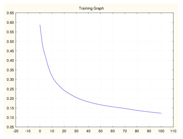
Figure 13.
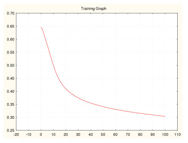
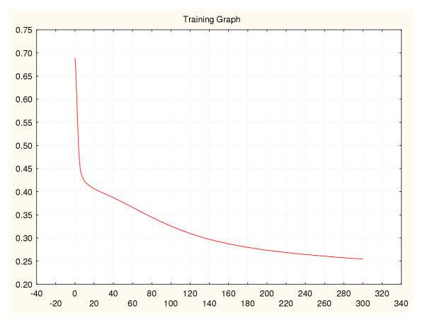
Mean square error during training for a leukaemia classifier (I) 50%–50% data splitting.
Figure 14.
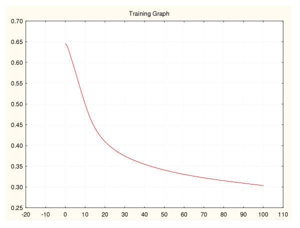
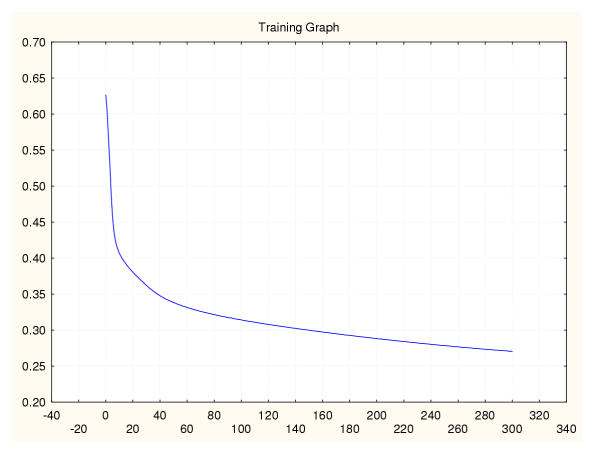
Mean square error during training for a leukaemia classifier (II) 75%–25% data splitting.
Figure 15.
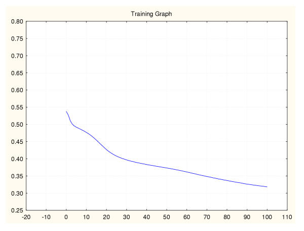
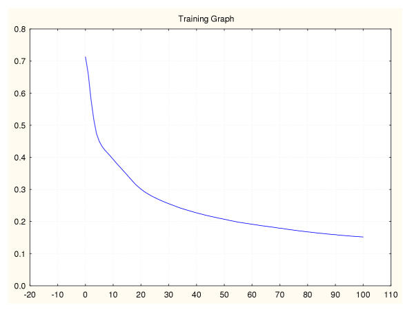
Mean square error during training for a leukaemia classifier (III) 95%–5% data splitting.
Figure 16.
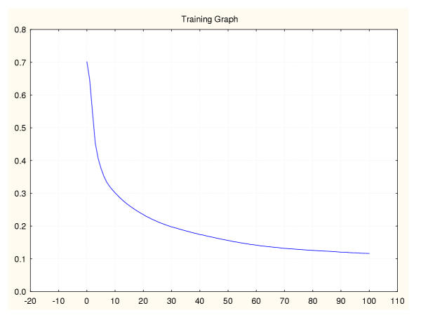
Mean square error during training for a leukaemia classifier (IV) Leave-one-out data splitting.
Figure 17.
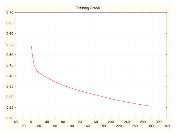
Entropy error during training for a SRBCT classifier (I) 50%–50% data splitting.
Figure 18.
Entropy error during training for a SRBCT classifier (II) 75%–5% data splitting.
Figure 19.
Entropy error during training for a SRBCT classifier (III) 95%–5% data splitting.
Figure 20.
Entropy error during training for a SRBCT classifier (IV) Leave-one-out data splitting.
Figure 21.
Entropy error during training for a splice-junction classifier (I) 50%–50% data splitting.
Figure 22.
Entropy error during training for a splice-junction classifier (II) 75%–5% data splitting.
Figure 23.
Entropy error during training for a splice-junction classifier (III) 95%–5% data splitting.
Figure 24.
Entropy error during training for a splice-junction classifier (IV) Leave-one-out data splitting.
The results originating from each sampling method and dataset are summarised in Tables 1 to 4. Tables 1, 2 and 3 compare the cross-validation results for the leukaemia, SRBCT and splice-junction datasets respectively. Table 4 summarises the bootstrap technique results.
Table 1.
Summary of cross-validation results for leukaemia data: Mean ± standard error of classification accuracies
| Train/test runs | 50%–50% cross validation | 75%–25% cross validation | 95%–5% cross validation |
| 10 | 0.786 ± 0.0176 | 0.844 ± 0.0319 | 0.775 ± 0.0583 |
| 25 | 0.760 ± 0.0149 | 0.804 ± 0.0225 | 0.730 ± 0.0477 |
| 50 | 0.732 ± 0.0117 | 0.763 ± 0.0164 | 0.735 ± 0.0306 |
| 100 | 0.725 ± 0.0083 | 0.744 ± 0.0125 | 0.750 ± 0.0213 |
| 500 | 0.736 ± 0.0033 | 0.764 ± 0.0049 | 0.770 ± 0.0093 |
| 1000 | 0.740 ± 0.0025 | 0.766 ± 0.0034 | 0.770 ± 0.0066 |
| 2000 | 0.739 ± 0.0018 | 0.764 ± 0.0024 | 0.768 ± 0.0048 |
| 3000 | 0.738 ± 0.0015 | 0.762 ± 0.0019 | 0.767 ± 0.0038 |
| 4000 | 0.740 ± 0.0013 | 0.762 ± 0.0017 | 0.770 ± 0.0033 |
| 5000 | 0.741 ± 0.0011 | 0.762 ± 0.0015 | 0.771 ± 0.0029 |
Table 4.
Summary of bootstrap method results for three datasets: Mean ± standard error of classification accuracies
| Train/test runs | Leukaemia | SRBCT | Splice-junctions |
| 100 | 0.743 ± 0.0108 | 0.753 ± 0.0074 | 0.965 ± 0.0014 |
| 200 | 0.736 ± 0.0078 | 0.741 ± 0.0057 | 0.962 ± 0.0011 |
| 300 | 0.738 ± 0.0062 | 0.740 ± 0.0044 | 0.960 ± 0.0009 |
| 400 | 0.739 ± 0.0053 | 0.740 ± 0.0038 | 0.961 ± 0.0007 |
| 500 | 0.742 ± 0.0047 | 0.741 ± 0.0033 | 0.960 ± 0.0007 |
| 600 | 0.742 ± 0.0042 | 0.744 ± 0.0030 | 0.962 ± 0.0006 |
| 700 | 0.743 ± 0.0039 | 0.745 ± 0.0028 | 0.961 ± 0.0006 |
| 800 | 0.744 ± 0.0035 | 0.746 ± 0.0026 | 0.961 ± 0.0006 |
| 900 | 0.746 ± 0.0033 | 0.746 ± 0.0024 | 0.961 ± 0.0005 |
| 1000 | 0.746 ± 0.0032 | 0.746 ± 0.0023 | 0.961 ± 0.0005 |
Table 2.
Summary of cross-validation results for SRBCT data: Mean ± standard error of classification accuracies
| Train/test runs | 50%–50% cross validation | 75%–25% cross validation | 95%–5% cross validation |
| 10 | 0.768 ± 0.0169 | 0.755 ± 0.0169 | 0.750 ± 0.0745 |
| 25 | 0.747 ± 0.0112 | 0.749 ± 0.0134 | 0.740 ± 0.0444 |
| 50 | 0.737 ± 0.0076 | 0.759 ± 0.0102 | 0.745 ± 0.0281 |
| 100 | 0.734 ± 0.0059 | 0.750 ± 0.0079 | 0.733 ± 0.0202 |
| 500 | 0.733 ± 0.0031 | 0.749 ± 0.0039 | 0.747 ± 0.0097 |
| 1000 | 0.732 ± 0.0021 | 0.752 ± 0.0027 | 0.749 ± 0.0068 |
| 2000 | 0.734 ± 0.0014 | 0.748 ± 0.0019 | 0.751 ± 0.0047 |
| 3000 | 0.733 ± 0.0012 | 0.749 ± 0.0016 | 0.758 ± 0.0038 |
| 4000 | 0.733 ± 0.0010 | 0.747 ± 0.0014 | 0.760 ± 0.0033 |
| 5000 | 0.733 ± 0.0009 | 0.746 ± 0.0012 | 0.761 ± 0.0030 |
Table 3.
Summary of cross-validation results for splice-junction sequence data: Mean ± standard error of classification accuracies
| Train/test runs | 50%–50% cross validation | 75%–25% cross validation | 95%–5% cross validation |
| 10 | 0.940 ± 0.0051 | 0.962 ± 0.0032 | 0.969 ± 0.0050 |
| 25 | 0.952 ± 0.0035 | 0.964 ± 0.0026 | 0.970 ± 0.0036 |
| 50 | 0.953 ± 0.0024 | 0.964 ± 0.0020 | 0.968 ± 0.0027 |
| 100 | 0.953 ± 0.0050 | 0.967 ± 0.0014 | 0.971 ± 0.0020 |
| 500 | 0.956 ± 0.0026 | 0.966 ± 0.0010 | 0.969 ± 0.0013 |
| 1000 | 0.957 ± 0.0019 | 0.968 ± 0.0008 | 0.969 ± 0.0011 |
| 2000 | 0.957 ± 0.0019 | 0.968 ± 0.0007 | 0.969 ± 0.0009 |
| 3000 | 0.958 ± 0.0016 | 0.966 ± 0.0007 | 0.968 ± 0.0014 |
| 4000 | 0.959 ± 0.0010 | 0.968 ± 0.0005 | 0.969 ± 0.0010 |
| 5000 | 0.957 ± 0.0009 | 0.968 ± 0.0005 | 0.970 ± 0.0008 |
Discussion
The assessment of classification performance is a crucial problem. Nevertheless, relatively little attention has been given to this problem in bioinformatics [8]. There is special concern in application domains, such as microarray data analysis, which have been based on the processing of relatively small datasets.
ANNs have become useful tools to assist several classification functions in genomic expression studies. A key problem is to determine the optimal amount of data required for both properly training the classifier and accurately estimating its predictive accuracy. In expression analysis, like in many other applications in biosciences, such an optimal solution is unknown. Moreover, this is difficult to estimate due to the limited size of the datasets available. Previous studies have addressed these issues in engineering and medical informatics applications [12,13].
In this paper, three sampling techniques were implemented to assess the classification accuracy of ANNs in three genomic data analysis problems. It shows that in general there is variability among the three techniques. However, these experiments suggest that it is possible to achieve lower variance estimates for different numbers of train-test runs. Furthermore, one may identify conservative and optimistic accuracy predictors, whose overall estimates may be significantly different. This effect is more distinguishable in small-sample applications.
For both expression datasets, the more conservative predictions were generated by the 50%–50% cross-validation and bootstrap methods. In the leukaemia classification problem, both methods require the same number of train-test experiments (1000) to significantly reduce the variance of their estimates. The estimates produced by such conservative classifiers were not significantly different. In the SRBCT classification task, the predictions generated by those methods were significantly different (t-tests, p < 0.01). However, they needed a similar number of train-test experiments to provide low variance estimates. The most optimistic estimates were produced by the 95%–5% cross-validation and leave-one-out techniques. Their accuracy estimates were not significantly different in both data classification problems.
The predicted accuracy of a classifier is generally proportional to the size of the training dataset. However, one of the reviewers of this paper has pointed out that the predicted accuracies for the leukaemia models increase little as the splits varies from 50%–50% trough 75%–25% to 95%–5%. The reviewer indicated that this may occur because some of the observations in the dataset may be considered as atypical, which has been reported by Golub and colleagues [14].
A larger dataset consisting of DNA splice-junction sequences was analysed in order to identify possible differences relating to the train-test data size factor. These classifiers were built on a more robust dataset. Therefore, the estimates generated by the sampling techniques are relatively similar. Like in the case of the expression data classification applications, the 50%–50% cross-validation and bootstrap methods produced the most conservative estimates. The most optimistic estimates were again provided by the 95%–5% cross-validation and leave-one-out techniques. There was a significant difference (t-tests, p < 0.05) between the lowest variance estimates generated by the bootstrap and the 95%–5% cross-validation methods. There were not significant differences between the most conservative approaches, and between the most optimistic approaches. Nevertheless, there are differences in terms of the number of train-test experiments required to reduce variability. In this problem, the leave-one-out method consists of 2000 train-test runs. The 95%–5% only requires 100 train-test runs to produce low variance estimates. Regarding the conservative accuracy classifiers: The 50%–50% cross-validation method may achieve low accuracy variability with 300 train-test experiments; the bootstrap method required at least 100 runs.
In general, the cross-validation results suggest that the classification accuracy estimates may increase when there is an increase in the size of the training dataset. Moreover, when the amount of testing data is reduced, more train-test data partitions are needed to achieve low variance estimates.
Previous research has indicated that the leave-one-out method may effectively address the problem of processing small datasets, due to its capability to process almost all of the available data for training the classifier. Overall, this method produced the highest accuracy estimates for the classification problems discussed here.
This study indicates that the bootstrap method may be applied to generate conservative and robust accuracy estimates, based on a relatively small number of train-test experiments.
Predicting the "true" accuracy of a classification approach is a complex and time-consuming problem. This type of analyses may be especially relevant to the development of more rigorous and reliable microarray data interpretation systems. This study may be benefited from the integration of alternative tools to visualise or measure classification performance [8,13].
There is a need to provide better insights into the process of evaluating the predictive capability of diagnostic and prognostic systems [8,15]. Future research should compare different classification approaches, including unsupervised methods [14]. Moreover, it will be important to have access to expression datasets comprising thousands of cases. Other important issues that deserve investigation are: The determination of relationships between data sampling techniques and feature selection methods, and the combination of multiple sampling techniques to produce more robust and reliable accuracy estimates.
Conclusions
This research suggests that, at least in the case of small expression datasets, thousands of train-test runs may be required to produce low variance performance predictions. Moreover, there may be differences among the estimates produced by different techniques. The results show that the 50%–50% cross-validation and bootstrap methods provide the most conservative estimates. Leave-one-out and 95%–5% cross-validation techniques generate the highest accuracy predictions. In comparison to other sampling techniques, the bootstrap method may require a small number of train-test experiments to produce low variance estimates. For datasets consisting of thousands of cases, a 95%–5% cross-validation procedure may be the best choice to achieve optimistic and low variance results, based on a relatively small number of train-test experiments.
The identification of the best sampling technique for the prediction of classification accuracy is a complex task. This problem, which has not been adequately studied by the bioinformatics community, may influence the outcomes of many tasks in biomedical research. The selection of a sampling technique will depend on the complexity of the application domain and the amount of data available. Another key issue that need to be carefully investigated is its relationship to feature selection.
This paper highlights the importance of performing more rigorous procedures on the selection of data and classification quality assessment. However, studies consisting of additional datasets and classification models are needed to recommend generic frameworks for the selection of data sampling techniques. This research may also be improved by applying more robust performance evaluation tools, such as receiver operating characteristic curves.
In general the application of more than one sampling technique may provide the basis for accurate and reliable predictions. A scientist may be more confident about the performance estimates if similar results are obtained by executing different techniques.
Methods
Data
The leukaemia data consisted of 72 cases categorised into two classes: Acute myeloid leukemia (AML) and acute lymphoblastic leukemia (ALL), which were represented by the expression values of 50 genes with suspected roles in processes relevant to these diseases. These classes included 25 and 47 cases respectively. The original datasets, experimental protocols and further analyses can be found in [13] and at the MIT Whitehead Institute Web site http://www.genome.wi.mit.edu/MPR.
The SRBCT data consisted of 88 cases categorised into four classes: Ewing family of tumors (EWS), rhabdomyosarcoma (RMS), Burkitt lymphomas (BL) and neuroblastomas (NB), which were represented by the expression values of 2308 genes with suspected roles in processes relevant to these tumors. Classes EWS, BL, NB and RMS contained 30, 11, 19 and 28 cases respectively. The original datasets, experimental protocols and further analyses can be found at the NHGRI Web site: http://research.nhgri.nih.gov/microarray/.
The splice-junction data consisted of 2000 sequences divided into three categories: Exon/intron boundaries (EI), intron/exon boundaries (IE) and neither (N). Each class comprised 464, 485 and 1051 cases respectively. Each case is represented by 60 features, which encode the nucleotide composition of each sequence based on a binary scheme. It uses 3 binary bits to represent each sequence base in the original data.
The original datasets and further information can be obtained at: http://www.liacc.up.pt/ML/statlog/datasets/dna/dna.doc.html.
Data preparation
Before training the networks the leukaemia expression data were normalised using the well known minimax technique. The dimensionality of the SRBCT expression samples was reduced by applying Principal Component Analysis (PCA). The 10 dominant PCA components for each case were used as the input to the classifiers as suggested by [6]. The 60 binary features representing each splice-junction sequence were used to train the networks without additional pre-processing.
Network architectures and training
All of the networks were trained with the Back Propagation algorithm. A learning epoch is defined as a single pass thorough the entire dataset. The learning stopping condition was based on the minimum improvement of error. In this method a training process is stopped if the classification performance (based on the sum-squared error or entropy function [12]) deteriorates for a number of learning epochs (the learning window). When training is stopped the best network found during training is preserved and included in the analyses.
The leukaemia data networks consisted of 50 input nodes, 5 hidden nodes and 2 outputs. They were trained during 100 learning epochs based on the sum-squared error function. The size of the learning window was equal to 5.
The SRBCT networks comprised 10 input nodes, 8 hidden nodes and 4 outputs. They were trained during 300 learning epochs based on the entropy error function. The size of the learning window was equal to 10.
The splice-junction sequence networks had 60 input nodes, 10 hidden nodes and 4 outputs. They were trained during 100 learning epochs based on the entropy error function. The size of the learning window was equal to 5.
The networks and sampling methods were implemented using the package Statistica™.
Sampling methods
For each train-test run, a classification accuracy value is predicted. The accuracy value for a particular train-test run is equal to the number of test cases correctly classified divided by the total number of test cases. For a set of train-test runs, for instance 100 or 1000 train-test runs, a mean accuracy value is calculated. Confidence intervals are then calculated for each mean. In this case, the 95 percent confidence interval is approximated with the mean plus or minus twice the standard error of the mean.
The author would like to state that the standard errors have been calculated on the basis that the runs are independent, which is an assumption that may not exactly hold in practice.
The accuracy values estimated for the train-test runs are assumed to be independent. It is supposed that the occurrence of each test accuracy value does not affect the occurrence or non-occurrence of the other test accuracy values. This is because the random sampling is performed with replacement. After a test dataset is selected and the classifier accuracy is evaluated, the test dataset is restored to the original dataset, and the whole dataset is shuffled. Thus, one may assume that each train-test run becomes independent of the previous sampling.
Even when different classifiers will be based on training and test datasets with observations in common, one assumes that their estimated classification accuracies are independent. That is because the probability of including a case, x, in the training (or test) dataset of the current train-test experiment is equal to the probability of including the same case, x, in the training (or test) dataset of the next train-test experiment.
In the cross-validation method the data is randomly divided into the training and test sets. This process is repeated several times and the classification performance is the average of the individual test estimates. In the leave-one-out method: Given n cases available in each dataset, a classifier is trained on (n-1) cases, and then is tested on the case that was left out. This process is repeated n times until every case in the dataset was included once as a cross-validation instance. For each classifier, the results were averaged across the n test cases to estimate the classifier's prediction performance. In the bootstrap method, a training dataset was generated by sampling with replacement n times from the available n cases. Each classifier is trained on the resulting set and then tested on the original dataset. This process is repeated several times, and the classifier's accuracy estimate is equal to the average of these individual estimates.
Acknowledgments
Acknowledgements
I thank the anonymous reviewers for helpful comments on this article.
References
- Welle S, Brooks AI, Thornton CA. Computational method for reducing variance with Affymetrix microarrays. BMC Bioinformatics. 2002;3:23. doi: 10.1186/1471-2105-3-23. [DOI] [PMC free article] [PubMed] [Google Scholar]
- Azuaje F. In Silico Approaches to Microarray-Based Disease Classification and Gene Function Discovery. Annals of Medicine. 2002;34:299–305. doi: 10.1080/078538902320322565. [DOI] [PubMed] [Google Scholar]
- Ideker T, Thorsson V, Ranish J, Christmas R, Buhler J, Eng J, Bumgarner R, Goodlett D, Aebersol R, Hood L. Integrated genomic and proteomic analyses of a systematically perturbated metabolic network. Science. 2001;292:929–933. doi: 10.1126/science.292.5518.929. [DOI] [PubMed] [Google Scholar]
- Bittner M, Meltzer P, Chen Y, Jiang Y, Seftor E, Hendrix M, Radmacher M, Simon R, Yakhini Z, Ben-Dor A, Sampas N, Dougherty E, Wang E, Marincola F, Gooden C, Lueders J, Glatfelter A, Pollock P, Carpten J, Gillanders E, Leja D, Dietrich K, Beaudry C, Berens M, Alberts D, Sondak V, Hayward N, Trent J. Molecular classification of cutaneous malignant melanoma by gene expression profiling. Nature. 2000;406:536–540. doi: 10.1038/35020115. [DOI] [PubMed] [Google Scholar]
- Azuaje F. A Computational neural approach to support the discovery of gene function and classes of cancer. IEEE Transactions on Biomedical Engineering. 2001;48:332–339. doi: 10.1109/10.914796. [DOI] [PubMed] [Google Scholar]
- Khan J, Wei J, Ringner M, Saal L, Ladanyi M, Westermann F, Berthold F, Schwab M, Antonescu C, Peterson C, Meltzer P. Classification and diagnostic prediction of cancers using gene expression profiling and artificial neural networks. Nature Medicine. 2001;7:673–679. doi: 10.1038/89044. [DOI] [PMC free article] [PubMed] [Google Scholar]
- Berrar D, Dubitzky W, Granzow M, editors Understanding and Using Microarray Analysis Techniques: A Practical Guide. London, Springer Verlag. 2002.
- Dougherty E. Small sample issues for microarray-based classification. Comparative and Functional Genomics. 2001;2:28–34. doi: 10.1002/cfg.62. [DOI] [PMC free article] [PubMed] [Google Scholar]
- Efron B, Gong G. A leisurely look at the bootstrap, the jack-knife and cross validation. American Statistician. 1983;37:36–48. [Google Scholar]
- Picard R, Berk K. Data splitting. American Statistician. 1990;40:140–7. [Google Scholar]
- Gong G. Cross-validation, the jackknife and the bootstrap excess error estimation in forward regression logistic regression. Journal of the American Statistical Association. 1986;81:108–13. [Google Scholar]
- Tourassi G, Floyd C. The effect of data sampling on the performance evaluation of artificial neural networks in medical diagnosis. Medical Decision Making. 1997;17:186–192. doi: 10.1177/0272989X9701700209. [DOI] [PubMed] [Google Scholar]
- Efron B, Tibshirani R. An Introduction to Bootstrap. New York, Chapman and Hall. 1993.
- Golub TR, Slonim D, Tamayo P, Huard C, Gassenbeck M, Mesirov JP, Coller H, Loh M, Downing J, Caligiuri M, Bloomfield C, Lander E. Molecular classification of cancer: class discovery and class prediction by gene expression monitoring. Science. 1999;286:531–537. doi: 10.1126/science.286.5439.531. [DOI] [PubMed] [Google Scholar]
- Azuaje F, Bolshakova N. Clustering Genome Expression Data: Design and Evaluation Principles. In: Berrar D, Dubitzky W Granzow M, editor. Understanding and Using Microarray Analysis Techniques: A Practical Guide. London, Springer Verlag; 2002. [Google Scholar]


