Thin-foil magnetic force system for high-numerical-aperture microscopy

Abstract

Forces play a key role in a wide range of biological phenomena from single-protein conformational dynamics to transcription and cell division, to name a few. The majority of existing microbiological force application methods can be divided into two categories: those that can apply relatively high forces through the use of a physical connection to a probe and those that apply smaller forces with a detached probe. Existing magnetic manipulators utilizing high fields and high field gradients have been able to reduce this gap in maximum applicable force, but the size of such devices has limited their use in applications where high force and high-numerical-aperture (NA) microscopy must be combined. We have developed a magnetic manipulation system that is capable of applying forces in excess of 700 pN on a 1 μm paramagnetic particle and 13 nN on a 4.5 μm paramagnetic particle, forces over the full 4π sr, and a bandwidth in excess of 3 kHz while remaining compatible with a commercially available high-NA microscope objective. Our system design separates the pole tips from the flux coils so that the magnetic-field geometry at the sample is determined by removable thin-foil pole plates, allowing easy change from experiment to experiment. In addition, we have combined the magnetic manipulator with a feedback-enhanced, high-resolution (2.4 nm), high-bandwidth (10 kHz), long-range (100 μm xyz range) laser tracking system. We demonstrate the usefulness of this system in a study of the role of forces in higher-order chromosome structure and function.

I. INTRODUCTION

Manipulators working on the cellular and subcellular levels provide a means for the investigation of the biomechanical properties essential for organisms to function. Among their numerous biological applications, such instruments have been used to deform cellular membranes,¹ probe intracellular properties,² and manipulate single biomolecules such as actin,^3,4 titin,^5,6 and DNA.^7-12 The wide range of forces necessary for these experiments, as well as the sensitivity requirements of the single-molecule experiments, greatly increases the difficulty in developing a manipulator that can adequately investigate the entire spectrum of possible experiments.

Measurement and application of forces at the nanoscale can be accomplished using multiple techniques. Among the mechanical probe techniques, glass fibers or microneedles^13-15 have been used to measure the effects of forces on the movement of chromosomes and the force exerted by myosin on actin.¹⁶ More recently, atomic force microscopy has emerged as a suitable method to obtain subnanometer spatial resolution¹⁷ with piconewton force sensitivity¹⁸ using techniques relying on the deformation of a cantilever spring element.¹⁹ In addition, Evans²⁰ has developed a method using a deformable vesicle attached to a pipette to measure the forces between membrane-bound molecules and target specimen such as other vesicles or flat substrates. While providing important insights within their domains, these methods suffer from the invasiveness of the attached fiber, cantilever, or pipette, as well as the inherent limitations in the sensitivity of the measurement [typically 10 pN for atomic force microscopy (AFM), 1 pN for micropipette²¹], and the number of directions that force may be applied.

To address these shortcomings, methods have been developed that use a refractive microbead, often below 1 μm in diameter, as a mechanical probe. The bead can be free to move throughout the accessible volume within a specimen or can be functionalized to be attached to specific molecular groups or proteins. Optical tweezers use the optical power gradient of a focused laser beam to attract refractive materials toward the waist of the focused beam.^22,23 The force generated on microbeads by the optical trap can be varied by changing the intensity of the laser and can be accurately calibrated.²⁴ Laser tweezers have been applied to a wide variety of biological problems, from measurements of the forces generated during DNA transcription,²⁵ to the properties of neuronal membranes,²⁶ and to the forces generated by the molecular motors dynein, kinesin, and myosin.^27-31 Additionally, laser tweezers have been used to study the mechanical properties of single molecules such as actin, DNA, and titin, and to investigate the forces required for nucleo-some disruption in chromatin.^32–37 This method offers increased sensitivity over the mechanical probe methods discussed above, with sensitivity down to approximately 0.1 pN.²¹ Its limitations are the achievable force (generally less than 200 pN), specimen heating at higher forces (approximately 10 °C/W of laser power at 1064 nm laser wavelength in water)^38,39 and the nonspecificity of forces which act on all refracting particles and macromolecules within the range of the optical trap. While laser heating is minimized with a trap using an 850 nm laser wavelength,⁴⁰ such lasers are not widely available at significant powers.

Using a magnetically permeable microbead and magnetic-field gradients, it is possible to perform manipulations similar to optical tweezers without the generation of specimen-damaging heat. In addition, since typical biological materials are at most weakly magnetically active, this method is more specific than optical tweezers. The sensitivity of this force-application method is limited by the detection system, the viscosity of the specimen, and the remnant magnetization of the magnetic materials. Typically magnetic systems can measure forces down to ≈0.01 pN.²¹

Beginning with Crick and Hughes⁴¹ in vitro studies of the viscoelastic properties of cytoplasm in 1949, magnetic forces have been used to investigate a wide range of biophysical properties. Many of the systems that have been reported have applied forces in a single direction, often with one pole tip.^42-45 Among these single-tip systems, Bausch et al. developed a device capable of applying up to 10 nN of force on a 4.5 μm paramagnetic bead.⁴⁵ Valberg and Albertini introduced a magnetic system designed for applying torques.⁴⁶ Strick et al. applied a multipole geometry to apply forces upward while applying a torque to a ferromagnetic bead.⁴⁷ Amblard et al.⁴⁸ introduced an eight-pole instrument whose construction was designed to apply torques as well as forces within the specimen plane. Haber and Wirtz¹² and Huang et al.¹ have both constructed systems designed to deliver a uniform gradient and allow for the use of a high-numerical-aperture (NA) objective. Huang implemented a full octapole design that utilized a backiron to complete the magnetic-flux circuit, resulting in increased field efficiency. Gosse and Croquette presented a six-pole design where the poles were located above the specimen with no magnetic forces available in the downward direction.¹⁰ This system also included optical tracking of the bead through the processing of images acquired by a camera. Our previous magnetic force prototype⁴⁹ consisted of a tetrapole design capable of applying forces in many directions, except those opposite the pole tips, as well as forces in the nanonewton range. This system used a stage-feedback-laser tracking system to provide bead position information over a 100×100×20 μm volume. The system we present here is a complete redesign and represents several advances over earlier designs, including that of our own. First, we have separated the pole tips from the flux-generating current coils, allowing easy reconfiguration of the field geometry at the sample. The pole tips are fabricated from thin foils, flattening the system geometry and allowing the use of high-NA objectives. Second, the bandwidth of the magnetics has been extended into the kilohertz range through the use of appropriate magnetic materials. Material considerations of prior designs were limited by the use of iron to bandwidths below 40 Hz due to eddy-current generation. Third, we demonstrate a system that can apply forces over the full 4π sr. With the bead near the pole tips, we have measured forces of over 700 pN on a 1-μm-diameter bead and over 13 nN on a 4.5-μm-diameter bead.

II. DESIGN OF THE INSTRUMENT

A. Force subsystem

1. Design considerations

Force on a magnetic bead is caused by the interaction between its magnetic dipole moment m and the gradient ∇B of an incident magnetic field. For a soft, magnetically permeable bead, m is entirely induced by the incident field. Subject to saturation properties of the magnetic material in the bead,

$$\mathit{m}=\frac{\pi d^3}{2{\mu }_0}\left(\frac{{\mu }_r-1}{{\mu }_r+2}\right)\mathit{B},$$

where μ₀ is the permeability of free space in Système International (SI) units, μr is the relative permeability of the bead, and d is the diameter of the bead. The magnetic force is

$$\mathbf{F}=\frac{\pi d^3}{4{\mu }_0}\left(\frac{{\mu }_r-1}{{\mu }_r+2}\right)\nabla \left(B^2\right).$$

The field is produced by multiple electromagnet pole tips arranged in space to provide the necessary directional capability. To optimize the magnitude of force, small tips are used to increase the gradient. Except very near a tip, its behavior can be modeled as a monopole, the field of which decreases quadratically with distance. Accordingly, the force depends on the inverse fifth power of distance from bead to tip. The force also depends quadratically on the B field, which in turn depends directly on electromagnet current and inversely on the size of air gaps between tips. These considerations motivate a small active region for magnetic forces and significant electromagnet coil currents.

2. Description of the magnetic system

The standard design for generating magnetic fields in a specimen is to couple the flux from a current-carrying coil to the sample region through a permeable core that narrows at the specimen. The coil is typically wound around the core, with the end closest to the specimen tapered to concentrate the flux so that a large field and a large field gradient are created. The analogy between electric circuits and magnetic circuits provides an immediate insight into magnetic system design. In a series electrical circuit it is obvious that, for a fixed voltage, the highest electric current will be produced when the circuit resistance is minimized. Using the magnetic-electrical circuit analogy, for a fixed magnetomotive force as generated by the current in the coils, the highest magnetic field will be produced when the circuit reluctance is minimized. This implies that the system should minimize air gaps and attempt to provide a high-permeability path for the flux through a return loop. We have included such a path in our system.

The circuit analogy provides a second insight. The magnetics system necessarily includes an air gap between pole tips at the specimen region. The reluctance of this gap is in series with other magnetic circuit reluctances, such as other gaps where the magnetic permeability is low. If the reluctance of these other gaps is significantly below that of the specimen air gap, then the total circuit reluctance, and hence magnetic performance, will not suffer. We have taken advantage of this freedom in design by separating the pole tips from the current-carrying coils and the flux return path. This provides flexibility in the implementation of a wide range of field geometries with facile exchange of pole tips. We provide for the ability to place magnetic pole tips above and below the specimen plane.

The fixed drivers consist of a pair of symmetrically opposed magnetic drive rings respectively above and below a specimen chamber. The use of a drive ring assures a completed magnetic-flux circuit, which is essential for efficient field use.¹ Each drive ring is a castellated annular magnetic core with a coil wound around each of its six castellations as shown in Fig. 4(c), thereby forming six drive poles. For the flux return path through the drive ring, we chose corrosion-resistant Metglas alloy 2417A (Honeywell, International Inc., Morriston, NJ) tape wound toroidal cores with a relative permeability of over 30 000 up to 30 kHz for field strengths above 0.01 T, a saturation induction of 0.57 T, and near-zero magnetostriction. After machining the six castellations in this material, coils were wound with 6×40 mil flat magnet wire, providing a high conductor fill ratio in the available space. In operation, the upper and lower drive-ring poles are precisely aligned with each other and with the pole plates. Corresponding upper and lower drive coils are connected in series to receive the same electrical current, such that their magnetic polarities are the same. This provides six magnetomotive excitations to drive magnetic flux into the pole plates.

FIG. 4.

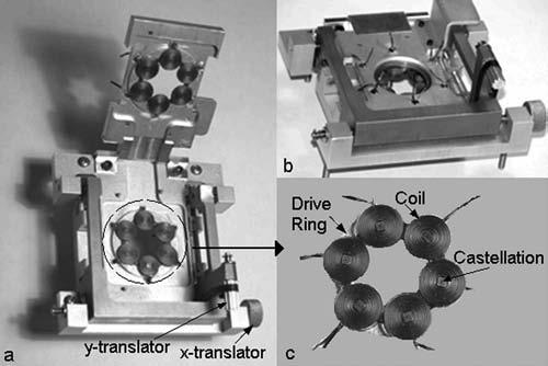
(a) Stage in open position showing double hinges, kinematic dowel pins, magnetic drivers, and xy-adjustable specimen slide holder. (b) Stage in closed position showing specimen chamber x and y adjustment knobs (no specimen chamber present). (c) A magnetic driver assembly comprising a drive ring and six coils. The drive ring is a laminated Metglas alloy 2714A (Honeywell, International Inc., Morriston, NJ) with high permeability, low magnetostriction and remanance, and excellent high-frequency performance. The coils are each 25 turns of 6×40 mil flat magnet wire for high fill factor. The design current is 2.5 A per coil.

The pole plates deliver magnetic flux from the drive rings to the specimen chamber. As shown in Fig. 1, they are necessarily thin to fit into the tightly constrained space limited by the close working distance of a high-NA microscope lens. A specimen can be placed directly on a pole plate, or in a separate coverslip sandwich that sits below one pole plate or in between two pole plates. The total thickness of the specimen+pole plate space can range from 150 to 500 μm. The upper drive ring is on a hinged mechanism, allowing it to be lowered onto the specimen chamber such that all the magnetic components are properly aligned. This provides for easily changing between experiment-specific specimen chambers without the need to change magnetic drivers. Specimen chambers may be selected from a standard library of configurations, or custom pole shapes and chambers can be fabricated for special purposes. Two example configurations we have studied are briefly described here and the results are presented in detail later.

FIG. 1.

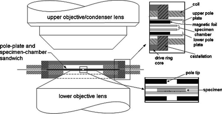
Vertically symmetric magnetic driver assembly consisting of drivering cores and coils, closely coupled to thin-foil poles in the pole-plate and specimen-chamber sandwich. The high-NA lower objective lens places tight geometric constraints on both sandwich and driver. A long-working-distance upper objective leaves space for other (e.g., microfluidic) subsystems.

A hexapole design, with a face-centered-cubic (fcc) pole tip placement around the specimen chamber, provides for nearly uniform three-dimensional (3D) force directionality over the full 4π sr of solid angle. Figure 2 shows how we implemented the fcc pole placement in two parallel planes, each containing three pole tips. In this configuration, a bead placed in the geometric center of the specimen chamber can be pulled over the full 4π sr with modest force.

FIG. 2.

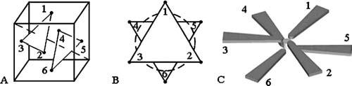
Implementation of a symmetric face-centered-cubic pole tip placement with thin-foil poles in two closely spaced parallel planes. (a) Optical axis (dashed line) is perpendicular to two planes, each containing three fcc points. (b) Two plates form parallel equilateral triangles with a cylindrical working volume between them. (c) Magnetic flux is conducted by thin-foil poles in two parallel planes to tips having centers at the fcc locations.

For cases where a force in only one direction is needed, a simple geometry is a single pole plate having one sharply pointed tip opposite a flat-nosed tip, with the bead located quite close to the sharp tip (Fig. 3). This configuration achieves high gradient near the sharply pointed tip, and high field strength at modest coil currents by a narrow gap between pole tips, augmented by the close proximity of the bead to the sharp tip.

FIG. 3.

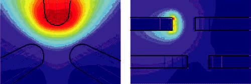
(Color) Simulation of field produced by one driven pole of the hexapole design. The field shape near the center of the specimen chamber is nearly spherical, justifying the validity of monopole models of the pole tips for calculating the force in that region.

Usability considerations require a mechanical stage to establish magnetic component alignment after a change of specimen chamber and to allow manual x-y adjustment of the specimen slide relative to the pole plates during experiment set up. We implemented this with a semikinematic design shown in Fig. 4(a). It uses a hinged upper plate to allow the upper drive ring to be lifted clear of the specimen chamber to provide access to the specimen or for changing it out entirely. In the closed position, the upper pole plate is constrained in z by adjustment screws (not shown). The pole plate(s) are kinematically positioned in x and y by three dowel pins anchored in the lower platform. The lower pole plate is constrained in z by the castellations of the lower drive ring. A specimen slide holder allows manual xy adjustment of the slide which is held at its corners by four rectangular locators, two of which are visible in Fig. 4(a).

3. Drive electronics

The drive amplifier is a six-channel transconductance amplifier, such that its output current is proportional to its input voltage. Its transconductance gain is 0.5 A/V. It was designed to drive a maximum of ±2.5 A per channel into a 5 μH inductive load typical of the three-dimensional force microscope (3DFM) drive coil operation. The small signal bandwidth driving a nominal load is 30 kHz. While it is stable for loads up to 50 μH, its full-power bandwidth of ≈10 kHz cannot be maintained for loads above 5 μH. The measured large-signal response to a triangle-wave input signal retains good linearity through 1 kHz with a 5 μH load. See Vicci⁵⁰ for a detailed description of the drive amplifier.

4. Pole materials and methods

Flux generated by the electromagnets is channeled towards the specimen region using pole plates that have been fabricated using two different methods. In the first method, pulsed electrodeposition^51-53 was used to deposit a magnetic material on the surface of a coverslip in a pattern described by a photolithography process. This method has the benefit of being able to develop complex pole geometries at the expense of processing complexity. The second method, laser machining of thin Permalloy foils (Laserod Inc., Gardena, CA), has been used to fabricate poles from commercially available magnetic foils. This process is capable of cutting materials with thicknesses up to ≈400 μm and offers 10 μm lateral resolution. Additionally, the use of commercially available materials ensures that the properties of the materials are well characterized. Figure 5(a) is a 175-μm-thick laser-machined three-pole pole plate. This is one-half of the hexapole geometry used in experiments, where the directionality of applied force is critical. Figure 5(b) is an example of the tip-flat geometry used to create high gradients for experiments where it is sufficient to pull in only one direction.

FIG. 5.

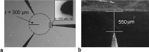
(a) Three-pole design using laser-machined pole pieces cut from 0.007-in.-thick low-permeability foil (Mushield). (b) Tip-flat geometry used in maximum force experiments.

B. Tracking subsystem

1. Design considerations

To determine the 3D location of the probe, we used a forward light-scattering technique⁵⁴ with little modification. This technique allows for full 3D particle tracking at rates limited only by the photodetector bandwidth, a rate that far exceeds the capabilities of video tracking. Unassisted, this technique has a working volume that is only on the order of the wavelength of the light used. To meet our long-range tracking requirements, we have implemented a feedback loop that dynamically repositions the particle to be inside this trackable volume. This capability is provided by adding a close-loop, active positioning stage driven by a control computer using active feedback to keep the particle within the optical tracker working volume.

2. Implementation

The available analytical models describing the mapping of quadrant photodiode (QPD) signals into XYZ positions relative to the beam waist^54,55 put stringent constraints on the shape, size, and composition of the tracked bead. For biological experiments that involve the application of force, beads of larger size are preferable to achieve a higher magnetic pull. Thus, we require more flexibility in probe characteristics than offered by an analytical model. As a result, we have developed a novel technique where, instead of relying on a priori model of the light scatter, we estimate the mapping function before (and potentially during) each experiment.

We use a standard system identification technique to determine the relationship between the QPD signals and bead position in three-dimensions. Before each experiment, small noise signals are injected into the three-axis piezodriven stage (model Nano-LP 100; Mad City Labs Inc., Madison, WI), causing the bead position to change in a calibrated manner. These small perturbations in the bead position result in small changes in the QPD signals. Correlations of the injected noise with corresponding photodiode signals are then analyzed to estimate the mapping function. The tracking software uses this newly estimated mapping function to improve its performance. A publication providing detailed information about the algorithm is in preparation.

C. System integration

The force and interferometric tracking subsystems have been added to an inverted optical microscope (model TE2000-E; Nikon Instruments, Melville, NY) that sits atop a 4×5 ft² vibration isolation table (model 78-249; Technical Manufacturing Corp., Peabody, MA).

The optics responsible for conditioning and steering the tracking laser (model IFLEX1000-P-2-830-0.65-35-N; Point Source, Southampton, England) sit behind the body of the microscope and are coupled into the light path using a custom dichroicmi that sits just beneath the objective. The optics associated with the interferometric tracking subsystem are presented in Fig. 6. For the feedback-enhanced tracking, the closed-loop, three-axis piezostage has been placed on top of the Nikon x-y translation stage. Feedback signals are obtained from a QPD (model QD-.05-0-SD; Centrovision, Newbury Park, CA), modified to have a 40 kHz cutoff frequency and a gain of 4.7×10⁵. The Nikon condenser assembly has been replaced by a custom unit that provides ridged arms for the mounting of the charge-coupled device (CCD) camera, QPD, and associated optics. XYZ translation of the custom condenser assembly is accomplished with commercial stages (XY axes: model ST1XY-S, Thorlabs, Newton, NJ; Z axis: model 443 series; Newport, Irvine, CA).

FIG. 6.

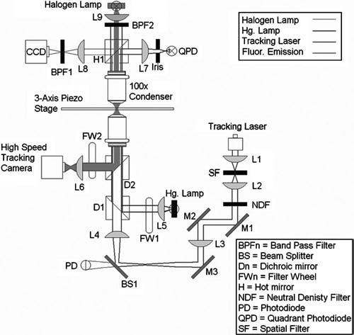
System optics. 825 nm, 36 mW fiber-coupled diode tracking laser is focused through a 10 μm spatial filter by lens L1. Lens L2 collimates the laser at the far side of the spatial filter before it passes through a neutral density filter (NDF 1) that decreases the optical power to 1.4 mW. The laser passes through the filter and onto mirror M1, which is responsible for axial translations of the laser beam through the rest of the lower optics system. Mirrors M2 and M3 steer the beam to BS1, which adjusts the angle of the beam entering the back of the objective. From BS1 the beam enters the back of the microscope, where D1 (dichroic) directs the beam vertically through the objective. Lenses L3 and L4 expand the beam twofold to slightly overfill the back aperture of the objective lens (model Plan Apo 60×/1.20 WI; Nikon Instruments Inc., Melville, NY). Laser light passing through the specimen (0.025 mW at specimen plane) is collected by a 100×, 0.7 NA air immersion Mitutoyo (model 378-806-2; Mitutoyo America Corporation, Aurora, IL) lens acting as the condenser. Hot mirror (H1) reflects longer wavelengths towards the QPD and allows the shorter wavelengths to pass. Lens L7 images the back focal plane of the objective onto the QPD (making the two conjugate pairs). Lens L8 forms a plane conjugate of the BFP of the condenser and the QPD for the purpose of imaging the diffraction pattern as seen by the QPD. BPF2 is an 830 nm bandpass filter designed to only let the tracking laser through to the CCD. This CCD is used for the centering of the bead's diffraction pattern on the QPD prior to the initiation of the tracking algorithm.

1. Computer control and data acquisition

The 3DFM system is controlled by five personal computers (PCs): one for the tracking subsystem; one for the magnet subsystem; one for high-resolution, high-speed video capture; one for low-resolution, low-speed video capture; and one for the user interface to the entire system. We elected to use several computers for aggregate processing power, convenience, and flexibility. For those that desire an inexpensive alternative, it would be possible to run both the magnet subsystem and a video-capture device from the same computer. Both the tracking and high-resolution/high-speed video-capture computers are based on workstation-class computers with dual 3 GHz Pentium Xeon processors, 1 Gbyte of main memory and 140 Gbytes of RAID0 disk. The tracking computer uses an analog output board (model PCI-6733; National Instruments, Austin, TX) for stage positioning, and a multifunction input-output ports (I/O) board for stage, QPD, and laser-intensity sensing (model PCI-6052E; National Instruments, Austin, TX). The high-resolution/high-speed video-capture computer controls a CoolSNAP HQ camera (Photometrics, Tucson, AZ) via a supplied peripheral component interconnect (PCI) card. The camera has a maximum resolution of 1392×1040 12-bit pixels digitized at 20 MHz. The magnet computer is desktop class with a 3 GHz Pentium4 processor and 512 Mbytes of main memory. A National Instruments analog output board (model PCI-6713) is used to drive the magnetics' electronics. Low-resolution/low-speed video capture is accomplished using a desktop-class computer with a 3 GHz Pentium4 processor and 512 Mbytes of main memory. The user interface computer is a workstation-class computer with dual 2.2 GHz Pentium Xeon processors, 1 Gbyte of main memory, and a Quadro4 (Nvidia, Santa Clara, CA) graphics card. The dual processors, large memory, and high-end graphics card are useful for computationally and display-intensive visualization tasks. The 3DFM user interface brings together several data streams from the microscope: bead trajectory, magnetic drive force, and two-dimensional (2D) fluorescent microscopy, and enables control over instrument parameters while displaying results from the instrument's subsystems.⁵⁶

III. RESULTS

A. System performance

1. Tracking resolution

The performance of the interferometric tracking subsystem has been tested using 0.957 μm polystyrene beads (Polysciences, Inc., Warrington, PA) immobilized in agarose. To test the system, a single bead was placed into the beam waist of the tracking laser. The bead was then moved by 4 nm square pulses in the positive x direction using the three-axis piezodriven stage. In Fig. 7, the QPD signal of the 4 nm displacement is shown for three different bandwidths of the measurement, i.e., 10 kHz, 1 kHz, and 100 Hz. From these experiments we have determined that the lateral resolution of the system is 2.4 nm at 10 kHz. A similar experiment for the axial resolution of the system resulted in a value of 4.4 nm at 10 kHz.

FIG. 7.

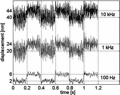
Tracking system response to 4 nm displacement. QPD signal for three bandwidths of the measurement, i.e., 10 kHz, 1 kHz, and 100 Hz, are shown. dc offsets were added to the 1 and 10 kHz data sets in the figure for clarity.

2. Magnetic forces

We determined the maximum forces generated by the magnetic system by measuring the velocity of 1 μm superparamagnetic beads and 4.5 μm superparamagnetic beads (M-450; Dynal Biotech, Oslo, Norway) in a 1600 cP 25 °C sucrose solution. The viscosity of this solution was measured using a commercial viscometer (model No. 513; Cannon Fenske, State College, PA). Particle velocities were determined using a video-tracking algorithm applied to brightfield images acquired using a 120 frames/s video camera. With the viscosity (η), bead radius (a_b), and bead velocity (ν), we can use Stokes formula, F=6πηa_bν, to calculate the magnetic force. Maximum force values of 700 pN and 13 nN were determined for the 1 and 4.5 μm beads, respectively, using a point-flat geometry with a 550 μm gap (see Fig. 5) made from a 350-μm-thick material with a saturation of approximately 20 000 Gauss and a permeability of 300 (MuShield, Mancheser, New Hampshire). This geometry was chosen for its simplicity and high field gradient near the pole tip. Force versus position data for 1 and 4.5 μm beads are displayed in Fig. 8.

FIG. 8.

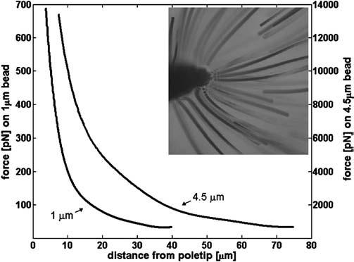
Maximum forces obtained on 1 and 4.5 μm superparamagnetic beads using a pole-flat geometry. Y axis corresponding to the force on the 4.5 μm bead is on the right-hand side of the figure. Insert image shows the paths of the 1 μm paramagnetic beads towards a pole tip during maximum force calibration experiment.

3. Magnetic system bandwidth

To determine the force bandwidth of the magnetic system, 1 μm superparamagnetic beads were oscillated in between opposite poles in a planar, six-pole geometry. Test frequencies were varied from 2 Hz to 4 kHz in a discrete manner. To account for the artifacts introduced by the motion of the bead relative to the poles, a control sinusoid was superimposed on each test frequency. The motion of the bead was followed by laser tracking and QPD signals were recorded at a sampling rate of ≈10 kHz. QPD signals were then mapped into XYZ position errors, which when added to the sensed positions of the three-axis piezostage give the displacement of the bead over time. The response to each test frequency was determined in four steps. First, we took PSD of the bead position over the time window over which excitation at that test frequency was applied. Second, we converted the height of the peak at the test frequency to bead response in terms of amplitude. Third, for the same time window, we computed the response to the control frequency in the same manner as that used for the test-frequency response. Finally, we normalized the response to test frequency by the response to the control frequency. This analysis revealed that the −3 dB roll off in the response function is greater than 3 kHz.

4. Magnetic force directionality

A hexapole design with a fcc pole tip placement around the specimen chamber can be used to provide nearly uniform 3D force directionality over the full 4π sr of solid angle. In our previous design using a tetrapole geometry, forces could not be applied in directions opposite the pole tips. Here we demonstrated the ability to pull in any direction in three dimensions through simulation and experiments. For the simulations, monopole approximations of the pole tips in the fcc hexapole design were used to model the field and field gradient generated by a given pole tip excitation. As a first step, this model was used to successfully verify full 3D force directionality by plotting 10 000 randomly generated pole tip excitations (not shown). The monopole approximation was also used in the development of an analytical bead force model⁵⁰ that can be used to generate a pole tip excitation that corresponds to a specified force vector. These calculated excitations were used to determine the relative values of the coil currents in the experimental verification of simulated results.

To verify the ability to pull in all directions, we first demonstrated large-scale magnetic symmetry by pulling a 2.8 μm superparamagnetic bead (M-280; Dynal Biotech, Oslo, Norway) towards each magnetic axis of symmetry [Fig. 9(a)]. This required a total of 26 different excitations: towards each of the six pole tips individually, between two adjacent poles, and between each set of three adjacent poles. For each of the 26 excitations, the pole tip was energized for 3 s, with the excitation order arranged so that the bead returned to the center of the geometry after every two excitations. In this experiment, movement in the expected direction is seen, but is off from the expected location by 6°–12° (depending on the axis of rotation). The deviation of the laboratory coordinate system from its theoretical location is most likely the source of this difference. Additionally, the measured maximum percent difference for the average force generated by one-, two-, and three-pole excitations was 31%, with an estimated average force of ≈1.5 pN. This average force could easily be increased to ≈15 pN for a 2.8 μm bead at the center of the geometry by reducing the distance from the center of the fcc geometry to each pole tip and increasing the coil currents.

FIG. 9.

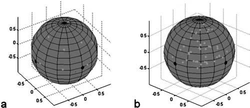
Experimentally obtained directional force data. The large black dots indicate pole locations and light grey dots indicate force directions (directions in which the bead was pulled). Axis of symmetry data (a) where forces were applied towards each pole, in between two poles, and in between three poles. (b) shows one octant of pole excitations.

Small-scale, fine control of bead position is demonstrated in Fig. 10(b). Here, force vectors were generated to sample the angle space between three poles, filling one octant of the surface of the sphere. Forces were applied in each direction for 3 s, with the bead being returned back to the origin after each excitation via a force in the opposite direction. The small-scale bead control (filling of the octant) shown in Fig. 9(b), combined with the symmetry data of the first experiment [Fig. 9(a)], indicates that we would be able to fill all eight octants on the surface of the sphere, and thus, pull the bead in all directions.

FIG. 10.

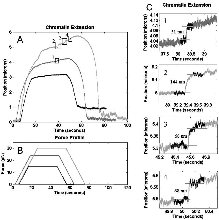
Chromatin extension: (a) Extension profile for three consecutive manipulations of the same chromatin fiber. For extensions where the maximum applied force was approximately 15 pN, no nucleosome disruption events were observed. In the subsequent traces (24 and 30 pN) the increased maximum force caused a total of four nucleosome disruption events [(c), 1–4], with possible multiple disruptions taking place in event 2. (b) Force profile corresponding to each extension in (a).

IV. 3DFM APPLICATION: CHROMATIN MANIPULATION

In addition to the experiments designed to show the 3DFM's ability to apply large forces and forces in full 3D, we have performed experiments that demonstrate the instrument's ability to obtain information from biological systems where both force and position sensitivities are key. In these experiments, chromatin fibers are extended with the goal of investigating the strength of the DNA-protein interactions that maintain the higher-order chromatin structure. The system is challenged to maintain nanometer-scale position-tracking sensitivity, while the bead moves over several microns. This is achieved using our stage-tracking routine that moves the nanometric specimen stage to keep the bead within the linear range of the laser tracking.

Chromatin, the condensed form of DNA, is made up of DNA and histone proteins. The association of DNA with these histones forms the nucleosome, a structure that condenses the DNA by wrapping it 1.65 times around a histone octomer. The histone octomer is made up of two copies of each of histone, H2A, H2B, H3, and H4, and is known as the nucleosome core particle (NCP).⁵⁷ Further compaction of the DNA is accomplished through interactions between core histone N-terminal domains and linker histones. This structure, and conformational changes that may take place throughout the cell cycle, is important to gene regulation and understanding the mechanisms behind transcription, replication, and repair.

A. Methods: Chromatin isolation and functionalization

Linearized lambda DNA (New England Biolabs, Beverly, MA; 48.5 kb) was labeled with digoxigenin-dUTP (Roche Molecular Biochemicals, Mannheim Germany) using the Klenow reaction (New England Biolabs). The DNA was then cut with XbaI and triple labeled with biotinylated dUTP (Roche Molecular Biochemicals) and biotinylated dATP and dCTP (Invitrogen Corp., Carlsbad, CA) using the Klenow reaction. Chromatin was formed from the DNA by incorporation of yeast nucleosomes using high-salt extraction of S. cerevisiae nuclear extracts, followed by a gradually decreased salt concentration to assemble nucleosomes onto the DNA. The chromatin was attached to the substrate using a digoxygenin/antidigoxygenin coupling on one side, with the second end attached to the magnetic bead using a stretavidin/biotin linkage, as desribed in the literature.³²

B. Results

Chromatin fibers were manipulated and extension (change in bead position) was monitored using the 3DFM and a “ramp and hold” manipulation method [Fig. 10(b)]. Fiber extension was monitored, with specific attention paid to sudden increases in overall extension (an indication of a possible nucleosome disruption event^34,35,58-60). Three consecutive extensions of the same fiber are shown in Fig. 10(a). For the initial application of force, where the maximum applied force was ≈15 pN, the tension on the nucleosome (histone-DNA complex) was not large enough to cause a disruption event. The overall extension of the chromatin fiber was significantly less (<50%) than what would be expected for b-form DNA alone, indicating that the nucleosome organization of the fiber remained intact. In the second extension of the fiber, with a maximum force of ≈24 pN, one nucleosome disruption event was observed during the “hold” interval [Fig. 10(c)]. The amplitude of the observed disruption events has been determined by taking the difference of the average of 1000 data points immediately before and 1000 data points immediately after the event. Using this method, the amplitude of this disruption event was determined to be 51 nm. For the third extension of the fiber (maximum force ≈30 pN), three nucleosome disruption events were observed, with amplitudes of 144, 68, and 68 nm for the first, second, and third events [Figs. 10(c2)-10(c4)]. Overall, the amplitude of the nucleosome disruption events shown in Fig. 10 are in reasonable agreement with published results for “full”³⁷ nucleosome disruptions, with the second disruption event most likely being the result of the removal of two nucleosomes.

It is important to note that the amplitude of the disruption events as observed by the 3DFM may be slightly larger than those viewed using traditional laser tweezers due to the inherent differences in these force-application methods. Traditional laser tweezers operate in a “position clamp” mode, where restorative forces act to maintain an object's position at the center of the laser trap. When the DNA that is wrapped around a nucleosome is released, it causes the force necessary to return the bead's position to the center of the laser trap to decrease, thus reducing the overall tension on the chromatin fiber. Manipulation techniques based on magnetics, such as the 3DFM, inherently operate in a “force clamp” mode, where force remains relatively constant as position changes. For these chromatin experiments, the constant force delivered by the 3DFM will extend the DNA released during a nucleosome disruption event slightly more than the reduced force of the laser trap. In addition, the constant force will allow for investigations into the cooperativity exhibited by nucleosome-nucleosome interactions, a property that would be indicated by increases in the number of multiple nucleosome disruption events.

This successful manipulation of chromatin, and our observation of multiple nucleosome disruption events at higher forces, demonstrates the utility of this system in biological investigations where both the range of applicable forces and the sensitivity of the position-detection system are key. Future improvements into the design of the instrument will focus on allowing the environmental conditions of the biological specimen, specifically the temperature and the properties of the media (i.e., salt concentration, protein concentration), to be altered through the course of an experiment while continuing to collect data. It will be most interesting to study protein reaction kinetics under an applied load. Since magnetics systems apply essentially no force to most unlabeled proteins, our system is ideally suited to force studies in the presence of protein solutions. Additionally, the bandwidth of the magnetic system will allow us to investigate the dynamic properties of viscoelastic materials, cells, and proteins.

References

- 1.Huang H, Dong CY, Kwon HS, et al. Biophys. J. 2002;82:2211. doi: 10.1016/S0006-3495(02)75567-7. [DOI] [PMC free article] [PubMed] [Google Scholar]
- 2.Hosu BG, Jakab K, Banki P, et al. Rev. Sci. Instrum. 2003;74:4158. [Google Scholar]
- 3.Kojima H, Ishijama A, Yanagida T. Proc. Natl. Acad. Sci. U.S.A. 1994;91:12962. doi: 10.1073/pnas.91.26.12962. [DOI] [PMC free article] [PubMed] [Google Scholar]
- 4.Liu XM, Pollack GH. Biophys. J. 2002;83:2705. doi: 10.1016/S0006-3495(02)75280-6. [DOI] [PMC free article] [PubMed] [Google Scholar]
- 5.Kellermayer MSZ, Smith SB, Bustamante C, et al. Biophys. J. 2001;80:852. doi: 10.1016/S0006-3495(01)76064-X. [DOI] [PMC free article] [PubMed] [Google Scholar]
- 6.Wang K, Forbes JG, Jin AJ. Prog. Biophys. Mol. Biol. 2001;77:1. doi: 10.1016/s0079-6107(01)00009-8. [DOI] [PubMed] [Google Scholar]
- 7.Bustamante C, Bryant Z, Smith SB. Nature (London) 2003;421:423. doi: 10.1038/nature01405. [DOI] [PubMed] [Google Scholar]
- 8.Bustamante C. Biophys. J. 2001;80:861. doi: 10.1016/S0006-3495(01)76064-X. [DOI] [PMC free article] [PubMed] [Google Scholar]
- 9.Strick TR, Allemand JF, Bensimon D, et al. Biophys. J. 1998;74:2016. doi: 10.1016/S0006-3495(98)77908-1. [DOI] [PMC free article] [PubMed] [Google Scholar]
- 10.Gosse C, Croquette V. Biophys. J. 2002;82:3314. doi: 10.1016/S0006-3495(02)75672-5. [DOI] [PMC free article] [PubMed] [Google Scholar]
- 11.Allemand JF, Bensimon D, Croquette V. Curr. Opin. Struct. Biol. 2003;13:266. doi: 10.1016/s0959-440x(03)00067-8. [DOI] [PubMed] [Google Scholar]
- 12.Haber C, Wirtz D. Rev. Sci. Instrum. 2000;71:4561. [Google Scholar]
- 13.Nicklas RB. J. Cell Biol. 1983;97:542. doi: 10.1083/jcb.97.2.542. [DOI] [PMC free article] [PubMed] [Google Scholar]
- 14.Schmitz KA, Holcomb-Wygle DL, Oberski DJ, Lindemann CB. Biophys. J. 2000;79:468. doi: 10.1016/S0006-3495(00)76308-9. [DOI] [PMC free article] [PubMed] [Google Scholar]
- 15.Yanagida T, Nakase M, Nishiyama K, et al. Nature (London) 1984;307:58. doi: 10.1038/307058a0. [DOI] [PubMed] [Google Scholar]
- 16.Skibbens RV, Salmon ED. Exp. Cell Res. 1997;235:314. doi: 10.1006/excr.1997.3691. [DOI] [PubMed] [Google Scholar]
- 17.Baker AA, Helbert W, Sugiyama J, et al. Biophys. J. 2000;79:1139. doi: 10.1016/S0006-3495(00)76367-3. [DOI] [PMC free article] [PubMed] [Google Scholar]
- 18.Florin E-L, Pralle A, Stelzer EHK, et al. Appl. Phys. A: Mater. Sci. Process. 1998;66:S75. [Google Scholar]
- 19.Braga PC, Ricci D. Methods in Molecular Biology. Vol. 242. Humana; Totowa, NJ: 2003. [Google Scholar]
- 20.Evans E. Annu. Rev. Biophys. Biomol. Struct. 2001;30:105. doi: 10.1146/annurev.biophys.30.1.105. [DOI] [PubMed] [Google Scholar]
- 21.Conroy RS, Danilowicz C. Contemp. Phys. 2004;45:277. [Google Scholar]
- 22.Ashkin A, Dziedzic JM, Bjorkholm JE, et al. Opt. Lett. 1986;11:288. doi: 10.1364/ol.11.000288. [DOI] [PubMed] [Google Scholar]
- 23.Block SM, Blair DF, Berg HC. Nature (London) 1989;338:514. doi: 10.1038/338514a0. [DOI] [PubMed] [Google Scholar]
- 24.Lang MJ, Block SM. Am. J. Phys. 2003;71:201. doi: 10.1119/1.1532323. [DOI] [PMC free article] [PubMed] [Google Scholar]
- 25.Yin H, Wang MD, Svoboda K, et al. Science. 1995;270:1653. doi: 10.1126/science.270.5242.1653. [DOI] [PubMed] [Google Scholar]
- 26.Dai JW, Sheetz MP. Biophys. J. 1995;68:988. doi: 10.1016/S0006-3495(95)80274-2. [DOI] [PMC free article] [PubMed] [Google Scholar]
- 27.Hirakawa E, Higuchi H, Toyoshima YY. Proc. Natl. Acad. Sci. U.S.A. 2000;97:2533. doi: 10.1073/pnas.050585297. [DOI] [PMC free article] [PubMed] [Google Scholar]
- 28.Block SM, Goldstein LS, Schnapp BJ. Nature (London) 1990;348:348. doi: 10.1038/348348a0. [DOI] [PubMed] [Google Scholar]
- 29.Kuo SC, Sheetz MP. Science. 1993;269:232. doi: 10.1126/science.8469975. [DOI] [PubMed] [Google Scholar]
- 30.Visscher K, Schnitzer MJ, Block SM. Nature (London) 1999;400:184. doi: 10.1038/22146. [DOI] [PubMed] [Google Scholar]
- 31.Rief M, Rock RS, Mehta AD, et al. Proc. Natl. Acad. Sci. U.S.A. 2000;97:9482. doi: 10.1073/pnas.97.17.9482. [DOI] [PMC free article] [PubMed] [Google Scholar]
- 32.Brower-Toland BD, Smith CL, Yeh RC, et al. Proc. Natl. Acad. Sci. U.S.A. 2002;99:1960. doi: 10.1073/pnas.022638399. [DOI] [PMC free article] [PubMed] [Google Scholar]
- 33.Claudet C, Angelov D, Bouvet P, et al. J. Biol. Chem. 2005;280:19958. doi: 10.1074/jbc.M500121200. [DOI] [PubMed] [Google Scholar]
- 34.Brower-Toland BDD, Yeh RC, Smith CL, et al. Biophys. J. 2002;82:907. [Google Scholar]
- 35.Bennink ML, Leuba SH, Leno GH, et al. Nat. Struct. Biol. 2001;8:606. doi: 10.1038/89646. [DOI] [PubMed] [Google Scholar]
- 36.Cui Y, Bustamante C. Proc. Natl. Acad. Sci. U.S.A. 2000;97:127. doi: 10.1073/pnas.97.1.127. [DOI] [PMC free article] [PubMed] [Google Scholar]
- 37.Pope LH, Bennink ML, van Leijenhorst-Groener KA, et al. Biophys. J. 2005;88:3572. doi: 10.1529/biophysj.104.053074. [DOI] [PMC free article] [PubMed] [Google Scholar]
- 38.Peterman E, Gittes F, Schmidt CF. Biophys. J. 2003;84:1308. doi: 10.1016/S0006-3495(03)74946-7. [DOI] [PMC free article] [PubMed] [Google Scholar]
- 39.Prasad PN. Opt. Lett. 2003;28:2288. doi: 10.1364/ol.28.002288. [DOI] [PubMed] [Google Scholar]
- 40.Schonle A, Hell SW. Opt. Lett. 1998;23:325. doi: 10.1364/ol.23.000325. [DOI] [PubMed] [Google Scholar]
- 41.Crick FHC, Hughes AFW. Exp. Cell Res. 1949;1:36. [Google Scholar]
- 42.Ziemann F, Radler J, Sackmann E. Biophys. J. 1994;66:2210. doi: 10.1016/S0006-3495(94)81017-3. [DOI] [PMC free article] [PubMed] [Google Scholar]
- 43.Assi F, Jenks R, Yang J, et al. J. Appl. Phys. 2002;92:5584. [Google Scholar]
- 44.Barbic M, Mock JJ, Gray AP, et al. Appl. Phys. Lett. 2001;79:1897. [Google Scholar]
- 45.Bausch AR, Ziemann F, Boulbitch AA, et al. Biophys. J. 1998;75:2038. doi: 10.1016/S0006-3495(98)77646-5. [DOI] [PMC free article] [PubMed] [Google Scholar]
- 46.Valberg PA, Albertini DF. J. Cell Biol. 1985;101:130. doi: 10.1083/jcb.101.1.130. [DOI] [PMC free article] [PubMed] [Google Scholar]
- 47.Strick TR, Allemand JF, Bensimon D, et al. Science. 1996;271:1835. doi: 10.1126/science.271.5257.1835. [DOI] [PubMed] [Google Scholar]
- 48.Amblard F, Yurke B, Pargellis A, et al. Rev. Sci. Instrum. 1996;67:818. [Google Scholar]
- 49.Fisher JK, Cummings JR, Desai KV, et al. Rev. Sci. Instrum. 2005;76 [Google Scholar]
- 50.Vicci L. Chapel Hill: 2005. (Report No. TR05-002). Department of Computer Science, University of North Carolina. unpublished. [Google Scholar]
- 51.Popov BN, Yin KM, White RE. J. Electrochem. Soc. 1993;140:1321. [Google Scholar]
- 52.Tang PT. Electrochim. Acta. 2001;47:61. [Google Scholar]
- 53.Osaka T, Takai M, Hayashi K, et al. Nature (London) 1998;392:796. [Google Scholar]
- 54.Pralle A, Prummer M, Florin EL, et al. Microsc. Res. Tech. 1999;44:378. doi: 10.1002/(SICI)1097-0029(19990301)44:5<378::AID-JEMT10>3.0.CO;2-Z. [DOI] [PubMed] [Google Scholar]
- 55.Rohrbach A, Stelzer EHK. Appl. Opt. 2002;41:2494. doi: 10.1364/ao.41.002494. [DOI] [PubMed] [Google Scholar]
- 56.Marshburn D, Weigle C, Wilde BG, et al. Proceedings of the IEEE Visualization 2005. IEEE Computer Society; Minneapolis, MN: 2005. [Google Scholar]
- 57.van Holde KE. Chromatin. Springer-Verlag; New York: 1988. [Google Scholar]
- 58.Pope LH, Bennink ML, Arends MP, et al. Biophys. J. 2002;82:2476. [Google Scholar]
- 59.Brower-Toland B, Wacker DA, Fulbright RM, et al. J. Mol. Biol. 2005;346:135. doi: 10.1016/j.jmb.2004.11.056. [DOI] [PubMed] [Google Scholar]
- 60.Leuba SH, Karymov MA, Tomschik M, et al. Proc. Natl. Acad. Sci. U.S.A. 2003;100:495. doi: 10.1073/pnas.0136890100. [DOI] [PMC free article] [PubMed] [Google Scholar]