Using Approximate Bayesian Computation to Estimate Tuberculosis Transmission Parameters From Genotype Data

Abstract

Tuberculosis can be studied at the population level by genotyping strains of Mycobacterium tuberculosis isolated from patients. We use an approximate Bayesian computational method in combination with a stochastic model of tuberculosis transmission and mutation of a molecular marker to estimate the net transmission rate, the doubling time, and the reproductive value of the pathogen. This method is applied to a published data set from San Francisco of tuberculosis genotypes based on the marker IS6110. The mutation rate of this marker has previously been studied, and we use those estimates to form a prior distribution of mutation rates in the inference procedure. The posterior point estimates of the key parameters of interest for these data are as follows: net transmission rate, 0.69/year [95% credibility interval (C.I.) 0.38, 1.08]; doubling time, 1.08 years (95% C.I. 0.64, 1.82); and reproductive value 3.4 (95% C.I. 1.4, 79.7). These figures suggest a rapidly spreading epidemic, consistent with observations of the resurgence of tuberculosis in the United States in the 1980s and 1990s.

TUBERCULOSIS (TB) is a directly transmitted disease caused by the bacterium Mycobacterium tuberculosis, which kills ∼2 million people each year. Much effort has been made to understand the patterns of transmission of TB in populations, for example, by constructing and analyzing deterministic epidemiological models. Properties of the population dynamics of the disease can also be investigated using estimates of the key parameters from epidemiological studies. This approach has led to a quantification of the intrinsic properties of the tuberculosis epidemic: the basic reproductive value (or R₀) of the disease is ∼4.5 (Blower et al. 1995) and it has a doubling time of 1–3 years (Porco and Blower 1998). Other measures of the extent or speed of transmission have also been studied, such as the risk of infection during a year or a lifetime (Garcia et al. 1997; Vynnycky and Fine 2000).

Genetic typing tools have helped to study the transmission of tuberculosis in populations and track particular chains of transmission. Common typing methods for characterizing the diversity of tuberculosis strains include insertion sequence (IS) typing (Cave et al. 1991) and spoligotyping (Kamerbeek et al. 1997). Insertion sequences are small bacterial transposable elements; IS6110 in particular transposes at a fast enough rate to allow effective discrimination of types within a set of clinical isolates of M. tuberculosis (Kremer et al. 1999). A DNA fingerprint based on IS6110 is generated by hybridization of the element to a Southern blot of a genome digested with a restriction enzyme that cuts once within each copy of the element. One advantage of the IS6110 marker system is that the rate at which genotypes change (the mutation rate) has been well studied (de Boer et al. 1999; Warren et al. 2002; Rosenberg et al. 2003). Strictly, the critical rate is the within-host substitution of new genotypes created by transposition, rather than transposition/mutation at the cellular level, but the term “mutation” is used here for simplicity. A major difference between these typing methods and DNA sequencing is that the latter allows the determination of the number of mutation events—through the number of segregating sites—while mutation events are often difficult to identify in the former.

To study transmission using genotype data, it is important to understand the mutation process at some level of detail. For example, one approach to estimating the extent of recent transmission is to count “clusters” of cases whose genotypes are identical, under the assumption that cases in the same cluster have arisen through recent transmission, as opposed to reactivation (Small et al. 1994). While a high proportion of cases in clusters should indicate a high level of recent transmission, we need to know the mutation rate to properly assess the impact of the clustering of genotypes in a sample. In other words, the clusteredness of genotypes can be attributed not only to fast transmission, but also to a slow mutation process. Ultimately, it would be useful to estimate transmission and other parameters formally by accounting for mutation, rather than summarizing data with indexes alone (Tanaka and Francis 2005). Although many studies use typing techniques such as these to measure the genetic diversity of TB isolates from particular geographic regions, little progress has been made in building theoretical foundations for analyzing the resulting data statistically.

Population parameters have been estimated from genetic data in other biological systems using appropriate models (e.g., Griffiths and Tavaré 1994; Kuhner et al. 1995, 2000; Tavaré et al. 1997; Pritchard et al. 2000; Drummond et al. 2002; Leman et al. 2005; Welch et al. 2005), but such efforts are sometimes hindered by difficulty in constructing analytical likelihood functions. Recent statistical advances allow Bayesian analyses while bypassing explicit likelihood functions by simulating data from the model. Indeed, the development of approximate Bayesian computation (ABC) has been motivated by population genetic problems. In these settings there are complex dependencies among individuals that can be simulated using the coalescent and related models, but likelihood functions are more difficult to write down (Marjoram et al. 2003). For a range of applications of methodologies that do not require likelihoods see Estoup et al. (2004), Tallmon et al. (2004), Hamilton et al. (2005), and Bortot et al. (2006).

The aim of this article is to devise a method to estimate appropriate (compound) parameters reflecting the transmission rate of a disease in a population, using a model of transmission, mutation, and sampling within a computational Bayesian framework. We first describe a simple stochastic model that includes both transmission of the disease and mutation of the marker and then provide a way to obtain the posterior distributions of compound transmissibility parameters using this model and genetic data. Applying the method to tuberculosis/IS6110 data from Small et al. (1994), we estimate the net transmission rate, the doubling time, and the reproductive value.

MODELS AND METHODS

A model of disease transmission and marker mutation:

A continuous-time stochastic model is used to describe the growth in the number of infectious cases of a disease over time. This model is an extension of the linear birth–death process. The “birth” component models the occurrence of new infections, while “death” corresponds to death or recovery of the host. To model the mutation process, we allow different genotypes of the pathogen. Note that mutation here assumes the replacement of one type with another within a host—that is, mutation as well as instantaneous fixation. Mutation between genotypes follows the infinite-alleles assumption: all mutation events give rise to genotypes that have never appeared before. We assume that all genotypes are selectively neutral with respect to each other—they all have the same epidemiological properties. In relation to the mutation and transmission processes, we assume that the processes are mutually independent, that the probability of each type of event over a short time interval is proportional to the number of cases, and that the process is time homogeneous so that the rates per individual remain constant over time. Finally we assume that the population is initiated with a single infection. The resulting model is similar to the birth–death and immigration model through which the distribution of family size can be studied (Tavaré 1989). The difference is that here the rate at which new types appear is proportional to the number of cases rather than being constant over time.

Let X_i(t) be the number of cases of genotype i and G(t) be the number of distinct genotypes that have existed in the population up to and including time t. Each of these random variables takes values from {0, 1, 2, … }. Let

be the total number of cases at time t.

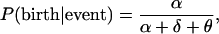
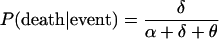
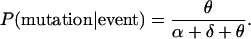
Define the following probabilities:

(1)

(2)

and

(3)

The three rates of the system are the birth rate α per case per year, the death rate δ per case per year, and the mutation rate θ per case per year. Under the assumptions given above, the time evolution of P_i,x(t) can be described by the differential equation

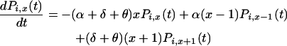(4)

for x = 1, 2, 3, … , and with boundary condition

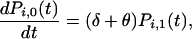where i represents any of the G(t) genotypes that have existed up to and including time t. For convenience, the genotypes are labeled i = 1, 2, 3, … , although the ordering has no meaning, except that i = 1 represents the parental type from which others are descended (directly or indirectly). The initial conditions are one copy of the ancestral genotype and no copies of any other genotype; that is, P_i,x(0) = 0 for all (i, x) except for P_1,1(0) = 1 and P_i,0(0) = 1 for i = 2, 3, 4, … . To account for the creation of new genotypes, the probability changes according to

and

(5)

with the condition that G(0) = 1. To establish the new genotypes, set P_g,1(t_g) = 1 and P_g,x(t_g) = 0 for x ≠ 1 for the time t_g at which genotype g first appears through mutation. Change in , concerning the total number of cases, is governed by the differential equations

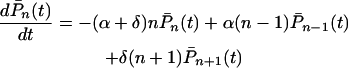(6)

for n = 1, 2, 3, … and

(7)

with initial conditions for n ≠ 1. This is a standard linear birth–death process. Note that the mutation process does not influence changes in the total number of cases.

Some properties of epidemics under the model:

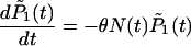
We first consider the theoretical properties of the epidemic regardless of the mutation process. The goal is to identify suitable functions of the parameters for estimation. Analysis of the full model including the generation of genetic variation is beyond the scope of this study; however, the total number of infectious cases N(t) follows a simple birth–death process. This section concerns some of the basic properties of this process (as defined by Equations 6 and 7) that can be found from the theory of stochastic processes (e.g., Feller 1968). The key quantities we estimate in this article are the net transmission rate, the doubling time, and the reproductive value.

Consider the dynamics of the total number of infectious cases. Let the expected total number be . Using the initial condition m(0) = N(0) = 1, the solution of this equation is

(8)

(see, for example, Karlin and Taylor 1975). Therefore α − δ, which we call the net transmission rate, is a key compound parameter describing the rate of increase of the number of cases in the population. Another associated parameter of interest is the doubling time, which for this model is ln(2)/(α − δ).

In analogy to deterministic models and branching process models of the spread of infectious diseases, we can define the reproductive number of the disease in a continuous-time transmission model as the expected number of new cases produced by a single infectious case while the primary case is still infectious. The “basic” reproductive value or R₀ is a related quantity corresponding to the situation where a single infection is introduced into a wholly susceptible population. Since the model we use does not explicitly track a susceptible population, we use the simpler term “reproductive value.” The use of the birth–death process here implicitly assumes a constant supply of susceptible people, an assumption that could be relaxed in more realistic models.

Consider a single infectious individual in a birth–death process. The time T until the death of a given individual is distributed exponentially with parameter δ. The probability density of this distribution is thus f_T(t) = δe^−δt. Let R be the number of new cases produced by a single infectious individual. In a linear birth–death process, this number is Poisson distributed with parameter αt where t is the duration of infectiousness. That is, the probability mass function is P(R = k | T = t) = e^−αt(αt)^k/k!, for k = 0, 1, 2, … . The unconditional distribution of the number of secondary cases R is therefore

and thus

The reproductive value in this model is therefore the ratio α/δ.

Simulation of the birth–death–mutation process:

This section describes the implementation of the computer simulation of the birth–death process with mutation. As mentioned above, we track three kinds of events, with rates α (birth), δ (death), and θ (mutation), X_i(t) is the number of cases of type i at time t, G(t) is the current number of distinct genotypes, and 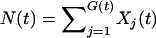is the total number of cases (of all types) at time t. To initialize the population X₁(0) is set to 1 and all other X_i(0) are set to zero; also, N(0) = 1 and G(0) = 1.

In this model, the time until the next event is distributed exponentially. The parameter of this distribution is the product of the total number of cases N(t) and the total rate of events of any kind, (α + δ + θ). However, we do not simulate these times since the total time experienced by the infectious population is not needed.

Given an event of one of the three kinds, the probability that it occurs in genotype i is X_i(t)/N(t). The probability of a birth event given that an event occurred is

and similarly,

If the event is a birth and the chosen genotype is i, the value of X_i(t) is incremented by 1. If the event is a death, the value of X_i(t) is decremented by 1. Note that if X_i(t) was zero, the probability of choosing i is zero, so its value cannot become negative. If the event is a mutation, the value of X_i(t) is decremented by 1, the value of G(t) is incremented by 1, and X_G(t)(t) is assigned the value 1. As discussed above, a mutation event always creates a new type.

If the population size N(t) reaches a prespecified number N_stop the process is stopped and a sample taken from it. The value of N_stop should reflect the size of a population carrying the appropriate level of diversity at the time the sample is taken. Low values of the order of 10³ with this model do not produce the appropriate level of diversity, while high values of the order of 10⁵ are in excess of realistic infectious population sizes in a given region. Among alternative values, N_stop = 10,000 gave high acceptance rates in the Bayesian computation; further, the outcomes are not strongly sensitive to changes in this parameter (results not shown). Samples of size n are drawn from the final population randomly without replacement. The clusters are of size n_i, where i = 1, 2, … , g and g is the number of distinct genotypes in the sample [in contrast to the whole population, in which there are G(t)]. If the population goes extinct, the simulation is discarded. In terms of the Bayesian analysis (see the following section) such a simulation is considered to give zero posterior probability to the parameters (α, δ, θ) from which it is generated.

Estimation of key quantities:

Data appropriate for the inference procedure described here consist of a set of clusters of size n_i where i = 1, 2, … , g and g is the number of distinct genotypes in the sample. The sample size is . Let D denote the data.

We adopt a Bayesian framework for parameter estimation, under which the posterior distribution p(α, δ, θ | D) = p(α, δ, θ)p(D | α, δ, θ)/p(D) is a normalized product of the prior and the (intractable) likelihood. The marginal posterior distribution of a parameter of the model, say α, is given by integrating out unwanted parameters:

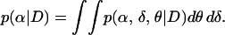However, as discussed above, combinations of α and δ produce parameters of biological interest. In particular, f₁(α, δ) = α − δ, f₂(α, δ) = ln(2)/(α − δ), and f₃(α, δ) = α/δ are of interest. We then require the posterior, for i = 1, 2, 3,

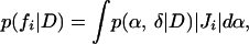where |J_i| is the Jacobian determinant of the change of coordinates from {f_i, α} to {δ, α}. Computing this distribution directly is unfeasible because the likelihood p(D | α, δ, θ) is unavailable, and the necessary integrations are intractable. Instead, we use approximate Bayesian computation because it does not require the likelihood to be known, only that simulation from the model is computationally inexpensive. The general approach is to approximate the likelihood through a distance metric defined on summary statistics between simulated and observed data.

The data can be summarized in a number of ways. A barrier to choosing appropriate statistics is the lack of knowledge about the sufficiency of possible statistics. For the infinite-alleles model, a diffusion model of genetic drift in which mutations follow the infinite-alleles assumption, Ewens (1972) showed that g is a sufficient statistic. However, we have a rather different population model here, and it is probably necessary to use information from other statistics. A biologically natural quantity to consider is the gene diversity

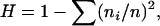which is related to heterozygosity in randomly mating diploid populations.

While a number of algorithms exist that implement approximate Bayesian inference (e.g., Beaumont et al. 2002), we adopt the method of Marjoram et al. (2003), which embeds the simulation process within the well-known Markov chain Monte Carlo (MCMC) framework. Define g* to be the number of distinct genotypes and H* to be the gene diversity statistic determined from a simulated sample. Let φ = (α, δ, θ) denote the vector of unknown parameters. The algorithm is as follows:

1. Initialize parameter values, φ₀. Set t = 0.

2. Propose a new set of parameter values φ* ∼ q(φ | φ_t) according to an arbitrary transition density q.

3. Simulate a sample of size n from the birth–death–mutation process using the proposed parameter values φ* and calculate the summary statistics g*, H*.

4. If , where ɛ is a suitably small threshold, and

   

   where u ∼ Uniform(0, 1), then set φ_t+1 = φ*. Otherwise set φ_t+1 = φ_t.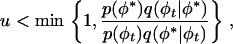

5. Set t = t + 1 and go to 2.

The above will generate a Markov chain φ₀, φ₁, φ₂, … whose stationary distribution is . Note that g and g* are normalized by dividing by n since they lie between 0 and n, while H and H* lie between 0 and 1. Following chain convergence, the parameter vectors form a (dependent) sample from this approximate joint posterior distribution. As in standard MCMC methods, the choice of the proposal density q(φ | φ_t) does not influence the stationary distribution of the chain, although it can affect its efficiency. Here it was specified as a multivariate normal whereby φ* ∼ N(φ_t, Σ) with covariance matrix

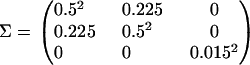The covariance of 0.225 between α and δ corresponds to a correlation of 0.9.

APPLICATION TO SAN FRANCISCO DATA

Prior specification:

Before discussing the data, we first address the prior specification. Since we wish to make inferences about α and δ from the data, we adopt an uninformative prior with respect to each of these parameters, such that both are positive and α > δ. In contrast, for the data in which we are interested, information is available in the literature about the mutation rate of some genetic markers. We therefore incorporate this external information into our analysis and specify

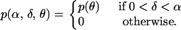This prior is improper (its integral is not 1), but this does not cause problems for the MCMC sampler of Marjoram et al. (2003) as all normalizing constants cancel out in the implied likelihood ratio.

A number of studies have attempted to estimate the mutation rate of IS6110 fingerprints. A study from the Netherlands (de Boer et al. 1999) gave an estimate of 0.2166/year (converted from a half-life estimate) with a 95% confidence interval of (0.13863, 0.33007). A study from South Africa (Warren et al. 2002) produced a much lower estimate of ∼0.08 (95% C.I. 0.066330, 0.092297). Another study used data from San Francisco and Germany (from Niemann et al. 1999) to obtain a per copy estimate of 0.0287 (Rosenberg et al. 2003). Extrapolating linearly, this estimate corresponds to a per strain rate of 0.287 for a strain with 10 copies, which is a typical copy number. However, the transposition rate as a function of copy number has been found to be nonlinear, with a peak value of ∼0.33 near 10 copies (Tanaka et al. 2004); hence the 0.287 number is likely to be an overestimate. Nevertheless, even with variation in these values, the point estimates lie within a fourfold range of each other. Taking into consideration this background information, we set the prior distribution for the mutation rate θ to be normal with mean 0.198 and standard deviation 0.06735 [i.e., p(θ) = N(0.198, 0.06735²)]. The mean was set to the average of 0.066 and 0.33, and the standard deviation was chosen such that the 95% limits of the distribution are 0.066 and 0.33.

Posterior distribution of key compound parameters:

We apply the methods of this study to the data of Small et al. (1994), an article that demonstrated the utility of the marker IS6110 in understanding the population dynamics of TB with molecular resolution. These data consist of 473 isolates collected in San Francisco during 1991 and 1992. The IS6110 fingerprints can be grouped into 326 distinct genotypes whose configuration into clusters can be represented by

where n^k indicates there were k clusters of size n.

The application of the approximate Bayesian computation method to the data of Small et al. (1994) produced informative posterior distributions on the compound parameters of interest. The Markov chain simulation was implemented for ∼2.5 million postconvergence iterations, retaining every 50th realization, with ɛ = 0.0025. The sensitivity of inference to the choice of ɛ is examined below.

Figure 1 shows the marginal posterior distribution of the net transmission rate α − δ, the doubling time ln(2)/(α − δ), and the reproductive value α/δ, and posterior estimates of these parameters are given in Table 1. The posterior distribution of the net transmission rate is almost symmetric, with a mean of 0.69 and a 95% credibility interval of (0.38, 1.08). The posterior of the doubling time shows essentially the same information, transforming it into units of interest in epidemiology. The mean doubling time is 1.08 years (95% C.I. 0.64, 1.82). The posterior distribution of the reproductive value α/δ is rather wide (95% C.I. 1.39, 79.7), with a heavy upper tail due to some positive posterior probability on very low values of δ. Most of the mass of the distribution, however, is near the median value of 3.43. The heavy tail suggests that the mean, which is ∼19, is too unstable to be used as a point estimate.

Figure 1.—

Marginal posterior densities of net transmission rate α − δ, doubling time log(2)/(α − δ), and reproductive value α/δ. The data used are from Small et al. (1994). The prior distribution of the mutation rate is p(θ) ∼ N(0.198, 0.06735²) and the tolerance level ɛ = 0.0025.

TABLE 1.

Posterior estimates of compound parameters from San Francisco data

Parameter	Description	95% credibility interval	Mean	Median
α − δ	Net transmission rate	(0.38, 1.08)	0.69	0.68
log(2)/(α − δ)	Doubling time	(0.64, 1.82)	1.08	1.02
α/δ	Reproductive value	(1.39, 79.71)	19.04	3.43

In the posterior distribution, the parameters α and δ are strongly correlated (ρ ≈ 0.85) as shown in Figure 2. This confirms that it is the relative values of these parameters that explain the observed data. The marginal posterior distribution of each individual parameter is therefore of little use on its own. The right side of Figure 2 reveals that the values of the net transmission rate that explain the data depend on the mutation rate. If the mutation rate is high, the net transmission rate must also be high to account for the diversity observed in the empirical sample.

Figure 2.—

Joint posterior densities p(α, δ | D) (integrating over θ) and p(α − δ, θ | D).

Sensitivity to mutation rate:

We present results from changing the mutation rate prior. Our inference relies on information about the mutation rate taken from the literature to “calibrate” the transmission rate estimation. Hence, it is important to know the effect of the assumed mutation rate prior distribution on the outcomes. We considered four different values of the mean around the adopted mean of 0.198, namely, 0.3, 0.25, 0.2, and 0.15. However, to study the effects of the location of the priors being different, we tightened the distributions through a reduction in standard deviation. Each prior had a standard deviation of 0.026, chosen so that the lower limits of the 95% prior credibility intervals of the distibutions with means 0.3 and 0.25 coincided, respectively, with the upper 95% limits of the distributions with means 0.2 and 0.15.

In Figure 3, we show the effect of varying the mutation prior on net transmission rate, doubling time, and reproductive value. The posterior reproductive value exhibits a remarkable resilience to the mutation rate: the ratio of birth to death rate is orthogonal to the mutation rate in the posterior distribution. In the left and middle of Figure 3 a higher mutation rate implies a higher net transmission rate and a lower doubling time. The standard deviation of the doubling time also decreases for a higher mutation rate. The superimposed posterior densities of the original analysis with p(θ) ∼ N(0.198, 0.06735²) indicate an averaging of the underlying uncertainty in the true value of the mutation rate.

Figure 3.—

Posterior densities of net transmission rate α − δ, doubling time log(2)/(α − δ), and reproductive value α/δ as prior mean of θ is varied. The prior means of θ are 0.15 (shaded dotted lines), 0.2 (shaded dashed lines), 0.25 (shaded solid lines), and 0.3 (dashed solid lines). The thick solid line corresponds to the analysis of Figure 1.

Tolerance level:

We investigated the effect of varying the tolerance parameter ɛ. This parameter affects both the computational efficiency and the accuracy of the inference. Unfortunately, with the Markov chain implementation of likelihood-free simulation, one can rarely be both efficient and accurate in the same analysis (other implementations have different drawbacks). The higher the value of ɛ, the greater the proportion of Metropolis–Hastings steps that are accepted and the faster the sampler moves around the parameter space. However, the fidelity of the posterior distribution to the observed data also becomes reduced. Conversely, a smaller tolerance implies lower acceptance rates, but improved data fidelity. While recent work (Bortot et al. 2006) suggests there may be a way to postpone specification of ɛ until examination of an augmented posterior distribution (which is also dependent on ɛ), we instead manually examine any differences in the posterior under a range of tolerance values.

Using the data of Small et al. (1994) and the prior on the mutation parameter p(θ) ∼ N(0.198, 0.06735²) we examined the series of ɛ-values: 0.025, 0.015, 0.005, and 0.0025. Sampler acceptance rates for these tolerances were 10.3, 5.9, 1.3, and 0.3%, respectively.

Figure 4 illustrates the effect of the tolerance parameter, in terms of sampler accuracy, on the net transmission rate, doubling time, and reproductive value. In each case there is a clear progression of densities as the tolerance is reduced. While we might hope that the posterior distributions stabilize beyond a certain tolerance value (i.e., when the information gained from decreasing its value becomes negligible), this does not appear to have occurred for the values trialed. Unfortunately a Markov chain with less than a 0.3% acceptance rate goes beyond acceptable time and computation limits for such a simulation (∼1 week on a computational cluster). Hence we acknowledge that while we have conducted this analysis to the limit of our computational power, the inference remains approximate. However, some speculative extrapolation may contend that, for example, the mode/median of the reproductive value α/δ might increase were we able to reduce ɛ further.

Figure 4.—

Posterior densities of net transmission rate α − δ, doubling time log(2)/(α − δ), and reproductive value α/δ as dependent on algorithm tolerance ɛ. The values of ɛ are 0.025 (shaded dashed lines), 0.015 (shaded solid lines), 0.005 (dashed solid lines), and 0.0025 (thick solid lines).

DISCUSSION

A useful though simple approach to studying TB genotype data is to analyze the proportion of isolates that appear in genetic clusters of size two or more (Alland et al. 1994; Small et al. 1994). These kinds of statistics serve to indicate the extent of recent transmission. A goal of the current study is to extract further information from TB genotype data by explicitly estimating transmission parameters from them. In particular, these parameters are estimated using a model of disease transmission and marker mutation along with a computational Bayesian method. In contrast to deterministic models of disease spread, we have used empirical data to estimate parameters, a methodology enabled by constructing a simple stochastic model. Bayesian methodology also has the advantage of incorporating parameter uncertainty directly within the inference and being able to assimilate expert information on quantities of interest from external sources. We have made use of these advantages, for example, by incorporating uncertainty in the mutation rate.

Our results indicate that in the data of Small et al. (1994) the reproductive rate of tuberculosis is ∼3.4, and the doubling time ∼1.1 years. The basic reproductive value of TB was previously estimated to be 4.5 (Blower et al. 1995), which is well within the credibility interval of the reproductive value in the present study. The posterior mean doubling time of 1.1 years in this study is low compared to the estimated 1–3 years of Porco and Blower (1998), although there is considerable overlap with the credibility interval. Although estimates of the rates of infection in the population (incidences) exist in the literature (Vynnycky and Fine 2000), estimates of the rates of transmission and recovery/death per infectious individual are unavailable, preventing any direct comparisons for the net transmission rate. However, the doubling-time estimate of 1–3 years (Porco and Blower 1998) corresponds to a range for the net transmission rate of 0.231–0.693/case/year, which encompasses our estimate of 0.69. Considering that the methods, models, and data used here are completely different from those in the work of Blower et al. (1995) and Porco and Blower (1998), it is interesting to observe that these estimates are not dissimilar to those previous estimates. Overall, the IS6110 data from San Francisco indicate a faster transmission than what has been put forward through general epidemiological studies. That is, the genetic information (as interpreted with the methods in this study) supports a faster spread of tuberculosis, at least for the data of Small et al. (1994). This conclusion agrees with the finding of that study that a large proportion of cases (around a third) were due to recent transmission and may reflect the strong transmission-driven resurgence of tuberculosis in urban populations in the United States in the 1980s and 1990s.

Interestingly, of the compound parameters estimated here, the reproductive value is the most robust to uncertainty in the prior distribution of the mutation rate. This suggests that the ratio of the birth to death parameters is of greater fundamental importance than the difference. This accords with intuition since the relative rates are what determine the outcome of events in the process.

Many details of tuberculosis epidemiology have been deliberately omitted from consideration to ask whether genotypes from molecular epidemiological studies alone can yield information about transmission. We have not included phenomena such as age structure, latent infection, reinfection, and migration; we also assume that the reproductive value of the pathogen is constant over time rather than varying as epidemiological circumstances change (Vynnycky and Fine 1998). We regard the estimated parameters as the “effective reproductive value,” “effective net transmission rate,” and “effective doubling time”—values that make the idealized model fit the data. Nevertheless, the statistical approach adopted here is an improvement on computing simple summary statistics from the data. Making use of further ideas from population genetics and computational Bayesian methods may help to refine our understanding of transmission patterns of TB. It may be worth developing more realistic models in the future, which include a larger number of parameters while still retaining the ability to recover the most important of these in the estimation procedure. If such models reflect TB dynamics effectively without using an excessive number of parameters, they may yield precise estimates of key parameters. Similarly, it is possible to increase the complexity of the mutation model to better capture the biology of the marker of interest. Here, we have been concerned with IS6110, but as other genetic typing systems such as spoligotyping and variable numbers of tandem repeats become more popular in the future, more specific mutation models can be incorporated into this methodology.

The advantages of approximate Bayesian computation to studies involving complex modeling are immense, as evidenced by a growing number of articles using this class of methods in population genetics (e.g., Hamilton et al. 2005). The approximate Bayesian computation approach enables the exploration of more realistic models without being hampered by the need to generate exact mathematical expressions for the likelihood function. In spite of this, a considerable challenge still remains in developing improved inferential procedures that reduce the effect of the “approximate” while keeping the “computation” to a manageable level. Several open problems include investigating how the degree of sufficiency of summary statistics can be efficiently determined, how to most effectively incorporate all simulations (with varying degrees of fidelity to the observed data) into the analysis, and the implications of choice of distance metric.

References

- Alland, D., G. Kalkut, A. Moss, R. McAdam, J. Hahn et al., 1994. Transmission of tuberculosis in New York City. An analysis by DNA fingerprinting and conventional epidemiologic methods. N. Engl. J. Med. 330: 1710–1716. [DOI] [PubMed] [Google Scholar]
- Beaumont, M. A., W. Zhang and D. J. Balding, 2002. Approximate Bayesian computation in population genetics. Genetics 162: 2025–2035. [DOI] [PMC free article] [PubMed] [Google Scholar]
- Blower, S. M., A. R. McLean, T. C. Porco, P. M. Small, P. C. Hopewell et al., 1995. The intrinsic transmission dynamics of tuberculosis epidemics. Nat. Med. 1: 815–821. [DOI] [PubMed] [Google Scholar]
- Bortot, P., S. G. Coles and S. A. Sisson, 2006. Inference for stereological extremes. J Am. Stat. Assoc. (in press).
- Cave, M. D., K. D. Eisenach, P. F. McDermott, J. H. Bates and J. T. Crawford, 1991. IS6110: conservation of sequence in the Mycobacterium tuberculosis complex and its utilization in DNA fingerprinting. Mol. Cell Probes 5: 73–80. [DOI] [PubMed] [Google Scholar]
- de Boer, A. S., M. W. Borgdorff, P. E. W. de Haas, N. J. D. Nagelkerke, J. D. A. van Embden et al., 1999. Analysis of rate of change of IS6110 RFLP patterns of Mycobacterium tuberculosis based on serial patient isolates. J. Infect. Dis. 180: 1238–1244. [DOI] [PubMed] [Google Scholar]
- Drummond, A. J., G. K. Nicholls, A. G. Rodrigo and W. Solomon, 2002. Estimating mutation parameters, population history and genealogy simultaneously from temporally spaced sequence data. Genetics 161: 1307–1320. [DOI] [PMC free article] [PubMed] [Google Scholar]
- Estoup, A., M. Beaumont, F. Sennedot, C. Moritz and J.-M. Cornuet, 2004. Genetic analysis of complex demographic scenarios: spatially expanding populations of the cane toad, Bufo marinus. Evolution 58: 2021–2036. [DOI] [PubMed] [Google Scholar]
- Ewens, W. J., 1972. The sampling theory of selectively neutral alleles. Theor. Popul. Biol. 3: 87–112. [DOI] [PubMed] [Google Scholar]
- Feller, W., 1968. An Introduction to Probability Theory and Its Applications, Vol. 1. John Wiley & Sons, New York.
- Garcia, A., J. Maccario and S. Richardson, 1997. Modelling the annual risk of tuberculosis infection. Int. J. Epidemiol. 26: 190–203. [DOI] [PubMed] [Google Scholar]
- Griffiths, R. C., and S. Tavaré, 1994. Simulating probability-distributions in the coalescent. Theor. Popul. Biol. 46: 131–159. [Google Scholar]
- Hamilton, G., M. Currat, N. Ray, G. Heckel, M. Beaumont et al., 2005. Bayesian estimation of recent migration rates after a spatial expansion. Genetics 170: 409–417. [DOI] [PMC free article] [PubMed] [Google Scholar]
- Kamerbeek, J., L. Schouls, A. Kolk, M. van Agterveld, D. van Soolingen et al., 1997. Simultaneous detection and strain differentiation of Mycobacterium tuberculosis for diagnosis and epidemiology. J. Clin. Microbiol. 35: 907–914. [DOI] [PMC free article] [PubMed] [Google Scholar]
- Karlin, S., and H. M. Taylor, 1975. A First Course in Stochastic Processes, Ed. 2. Academic Press, San Diego.
- Kremer, K., D. van Soolingen, R. Frothingham, W. H. Haas, P. W. Hermans et al., 1999. Comparison of methods based on different molecular epidemiological markers for typing of Mycobacterium tuberculosis complex strains: interlaboratory study of discriminatory power and reproducibility. J. Clin. Microbiol. 37: 2607–2618. [DOI] [PMC free article] [PubMed] [Google Scholar]
- Kuhner, M. K., J. Yamato and J. Felsenstein, 1995. Estimating effective population size and mutation rate from sequence data using Metropolis-Hastings sampling. Genetics 140: 1421–1430. [DOI] [PMC free article] [PubMed] [Google Scholar]
- Kuhner, M. K., J. Yamato and J. Felsenstein, 2000. Maximum-likelihood estimation of recombination rates from population data. Genetics 156: 1393–1401. [DOI] [PMC free article] [PubMed] [Google Scholar]
- Leman, S. C., Y. Chen, J. E. Stajich, M. A. F. Noor and M. K. Uyenoyama, 2005. Likelihoods from summary statistics: recent divergence between species. Genetics 171: 1419–1436. [DOI] [PMC free article] [PubMed] [Google Scholar]
- Marjoram, P., J. Molitor, V. Plagnol and S. Tavaré, 2003. Markov chain Monte Carlo without likelihoods. Proc. Natl. Acad. Sci. USA 100: 15324–15328. [DOI] [PMC free article] [PubMed] [Google Scholar]
- Niemann, S., E. Richter and S. Rusch-Gerdes, 1999. Stability of Mycobacterium tuberculosis IS6110 restriction fragment length polymorphism patterns and spoligotypes determined by analyzing serial isolates from patients with drug-resistant tuberculosis. J. Clin. Microbiol. 37: 409–412. [DOI] [PMC free article] [PubMed] [Google Scholar]
- Porco, T. C., and S. M. Blower, 1998. Quantifying the intrinsic transmission dynamics of tuberculosis. Theor. Popul. Biol. 54: 117–132. [DOI] [PubMed] [Google Scholar]
- Pritchard, J. K., M. Stephens and P. Donnelly, 2000. Inference of population structure using multilocus genotype data. Genetics 155: 945–959. [DOI] [PMC free article] [PubMed] [Google Scholar]
- Rosenberg, N. A., A. G. Tsolaki and M. M. Tanaka, 2003. Estimating change rates of genetic markers using serial samples: applications to the transposon IS6110 in Mycobacterium tuberculosis. Theor. Popul. Biol. 63: 347–363. [DOI] [PubMed] [Google Scholar]
- Small, P. M., P. C. Hopewell, S. P. Singh, A. Paz, J. Parsonnet et al., 1994. The epidemiology of tuberculosis in San Francisco: a population-based study using conventional and molecular methods. N. Engl. J. Med. 330: 1703–1709. [DOI] [PubMed] [Google Scholar]
- Tallmon, D. A., G. Luikart and M. A. Beaumont, 2004. Quantitative evaluation of a new effective population size estimator based on approximate Bayesian computation. Genetics 167: 977–988. [DOI] [PMC free article] [PubMed] [Google Scholar]
- Tanaka, M. M., and A. R. Francis, 2005. Methods of quantifying and visualising outbreaks of tuberculosis using genotypic information. Infect. Genet. Evol. 5: 35–43. [DOI] [PubMed] [Google Scholar]
- Tanaka, M. M., N. A. Rosenberg and P. M. Small, 2004. The control of copy number of IS6110 in Mycobacterium tuberculosis. Mol. Biol. Evol. 21: 2195–2201. [DOI] [PubMed] [Google Scholar]
- Tavaré, S., 1989. The genealogy of the birth, death and immigration process, pp. 41–56 in Mathematical Evolutionary Theory, edited by M. W. Feldman. Princeton University Press, Princeton, NJ.
- Tavaré, S., D. J. Balding, R. C. Griffiths and P. Donnelly, 1997. Inferring coalescence times from DNA sequence data. Genetics 145: 505–518. [DOI] [PMC free article] [PubMed] [Google Scholar]
- Vynnycky, E., and P. E. Fine, 1998. The long-term dynamics of tuberculosis and other diseases with long serial intervals: implications of and for changing reproduction numbers. Epidemiol. Infect. 121: 309–324. [DOI] [PMC free article] [PubMed] [Google Scholar]
- Vynnycky, E., and P. E. Fine, 2000. Lifetime risks, incubation period, and serial interval of tuberculosis. Am. J. Epidemiol. 152: 247–263. [DOI] [PubMed] [Google Scholar]
- Warren, R. M., G. D. van der Spuy, M. Richardson, N. Beyers, M. W. Borgdorff et al., 2002. Calculation of the stability of the IS6110 banding pattern in patients with persistent Mycobacterium tuberculosis disease. J. Clin. Microbiol. 40: 1705–1708. [DOI] [PMC free article] [PubMed] [Google Scholar]
- Welch, D., G. K. Nicholls, A. Rodrigo and W. Solomon, 2005. Integrating genealogy and epidemiology: the ancestral infection and selection graph as a model for reconstructing host virus histories. Theor. Popul. Biol. 68: 65–75. [DOI] [PubMed] [Google Scholar]