


Abstract
Microarray or DNA chip technology is revolutionizing biology by empowering researchers in the collection of broad-scope gene information. It is well known that microarray-based measurements exhibit a substantial amount of variability due to a number of possible sources, ranging from hybridization conditions to image capture and analysis. In order to make reliable inferences and carry out quantitative analysis with microarray data, it is generally advisable to have more than one measurement of each gene. The availability of both between-array and within-array replicate measurements is essential for this purpose. Although statistical considerations call for increasing the number of replicates of both types, the latter is particularly challenging in practice due to a number of limiting factors, especially for in-house spotting facilities. We propose a novel approach to design so-called composite microarrays, which allow more replicates to be obtained without increasing the number of printed spots.
INTRODUCTION
Oligonucleotide arrays (1,2), both synthesized and spotted, enjoy several advantages over cDNA-based arrays (3,4), such as simpler methodology to obtain DNA and better quality control, options to select high-specificity sequences to avoid cross-hybridization, and the potential to detect alternative spliced variants of genes (5). It is known that microarray gene expression measurements exhibit both between-slide and within-slide variability (6) and that apart from making efforts to improve the technology, having replicate measurements is essential for improving the reliability of subsequent quantitative analysis. Dealing with between-slide variability involves repeating entire microarray experiments. There exist some limitations, however, such as availability of RNA as well as cost factors. To address within-slide variability, the typical approach entails printing replicate spots on the same slide. However, spotting robots typically have a limitation on the number of spots that can be reliably printed. Thus, increasing the number of replicates can be done at the expense of decreasing the number of genes surveyed. In addition, even if the total number of spots was not a limitation, having more spots requires more labor during the image analysis stage, as most microarray image analysis tools are not totally unsupervised or automatic, which translates directly into higher cost or lower throughput. Finally, fewer spots require less physical space on the solid support (e.g. glass slide), which in turn translates into smaller amounts of RNA required for hybridization.
The primary reason for the above tradeoffs is rooted in the fact that current spotted microarray technology employs one printed spot per measurement. Although the ‘one spot–one gene’ methodology is straightforward to implement and appealing from the standpoint of visual inspection of the produced images, where specific genes of interest can quickly be qualitatively examined without further analysis, it is not necessarily the most efficient.
If we think of the spotted DNA that corresponds to some particular gene as a signal and of the spot itself as a sensor or receiver, then the standard microarray approach entails using one sensor (spot) to detect only one signal (gene). This scenario is illustrated in Figure 1a. A more general approach would be to allow each sensor to detect more than one signal. That way, each signal is received and recorded at several different sensors simultaneously. For example, Figure 1b depicts the situation where each spot is used to detect two different genes. Such a set-up is called a sensor array and has been extensively used in radar and sonar signal processing, where antenna arrays are used (7), in electroencephalography and magnetoencephalography, where a number of electrodes are simultaneously recording brain activity (8), in remote sensing (9), and in other applications. In molecular biology, a similar approach has been used for high-throughput genotyping (10). For example, suppose several people are speaking simultaneously in the same room while several microphones, positioned in different locations, are simultaneously recording the conversations. Thus, each microphone receives a typically linear mixture of several different signals. The task is to recover the original signals (speakers) from the recorded mixtures. This problem is called the blind source separation problem and has received a considerable amount of attention in the signal processing community (11,12).
Figure 1.
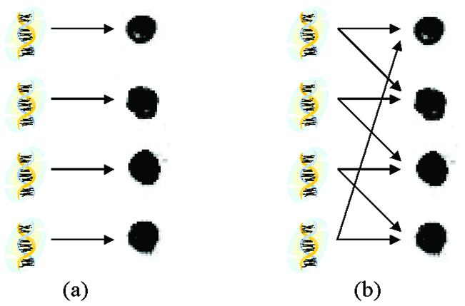
An illustration of the difference between the standard and proposed approaches to microarray design. The drawing in (a) shows that each gene represented in an oligonucleotide (oligo) is placed into its own individual spot on the glass slide. Drawing (b) shows an example where each spot contains a mixture of two different oligos. Thus, it is expected that the measured signal intensity of such a spot would be a combination of the intensities of the constituent genes measured individually.
The approach that we propose here is quite similar in spirit to the above problem and consists of spotting a mixture of two or more oligos into the same spot. The challenge then is to recover the individual gene intensities by observing the intensities of the mixtures. This is, in fact, conceptually simpler than the blind source separation problem because we know exactly which genes are present in which spots and because intensities are simply scalars and not time-varying signals. In addition, the contributions from the mixed oligos are expected to be mutually independent, as they are designed to be non-homologous to each other, which is a fundamental assumption of all oligonucleotide microarrays. The obvious benefit of this approach is that each gene is given an opportunity to make several contributions in different spots, each time with a different partner, and therefore, is also a type of replication. The question is whether the original gene expressions can be reliably recovered from such mixtures.
MATERIALS AND METHODS
Oligonucleotide design
For the proof-of-principle experiments, we designed 30 oligonucleotides (oligos) of 50 bases in length representing 30 genes that are expressed at different levels in the colon carcinoma cell line RKO (ATCC, CRL-2577). The 50-base oligonucleotide for each gene was from within the 500 bp of the 3′ end of each of the cDNA and had minimal homology with any other genes in the BLAST search. The accession numbers for the 30 genes are: X00351, X01677, K00558, L20941, NM_002283, NM_007260, NM_004798, NM_003192, NM_003747, NM_014328, NM_018728, U90942, NM_005619, NM_002278, M11147, NM_002274, M86400, NM_001016, L06505, U14971, V00530, X98507, NM_006709, X16302, AF019770, L25610, L26165, NM_000595, NM_000594, T95289.
Oligo mixing
Oligos were combined on a RSP100 liquid handling robot (Tecan Systems, San Jose, CA). For single spots, 0.825 µg of each oligo was transferred into five wells of a 384-well plate. For mixed oligos, 0.825 µg of each of the partner oligos was transferred to the same well. This pair was repeated for five positions. The 384-well plates were dried and the oligos in each well were resuspended in 1 µl of 50% DMSO array buffer (50 µM for each oligo).
Spotting
Oligos were spotted onto poly-l-lysine glass slides by a G3 solid pin spotter (Genomic Solutions, Ann Arbor, MI, USA), baked at 65°C for 90 min, and crosslinked with 65 mJ of ultraviolet radiation.
Probe labeling, hybridization and quantification
The microarray experiments were performed as described previously (13). Briefly, triplicate reverse transcription reactions using 100 µg of total RNA from RKO cells incorporated Cy3 d-CTP into cDNA. After G50 column purification, replicates were combined for uniformity and distributed to three identical microarray slides. Each slide was hybridized overnight at 60°C in a humid incubator, then washed at 37°C with increasing stringency until 0.1× SSC was used. Slides were scanned on a LSIV laser scanner (Genomic Solutions, Ann Arbor, MI, USA) and quantified using ArrayVision software (Imaging Research, Inc, St Catherine’s, Ontario, Canada).
RESULTS
Our experiment consisted of designing a spotted microarray containing 30 genes represented in 50 bp oligos that are expressed at different levels in RKO colon cancer cells based on our prior experiments. Those genes were spotted individually five times each, as well as mixtures of all possible pairs of genes, for a total of (30 × 29) / 2 = 435 pairs. Thus, each of the 30 genes appeared 29 times with different partner genes. Finally, each mixture was replicated five times to facilitate statistical analysis. Total RNA was isolated from RKO colon cancer cells and used for microarray experiments.
As a first step, we proceeded to discover how the intensities of signals of the mixtures are related to signal intensities of the individual genes. Prior to any experimentation, it was expected that the intensity of the mixture should be at least an increasing function of the individual intensities. In other words, the higher the expression of the two genes, the higher is the signal from their mixture. It was further anticipated that the mixture would be a linear combination of the individual gene intensities. That is, if xi is the individual intensity of gene i, xj is the intensity of gene j ≠ i, and yk(i,j) is the intensity of the mixture of genes i and j, then yk(i,j) = a(xi + xj) + n, i, j, = 1, ..., 30, for some scalar a and additive error component n. Here, k(i, j) is simply an index that counts from 1 to 435, so k(1, 2) = 1, k(1,3) = 2, ..., k(29,30) = 435. Note that since genes are simply mixed in equal proportions, there is no notion of ‘first’ or ‘second’ gene and thus, we would not expect different weights ai and aj for genes xi and xj. Also, for the least-squares approach that we use below, no statistical description of the error component n is required. Rewriting the above relationship in vector-matrix notation, we have:
y = aAx + n
where y is a 435 × 1 vector of mixtures, x is a 30 × 1 vector of individual gene intensities, A is a binary matrix of size 435 × 30 in which row k(i, j) contains ones in the ith and jth positions and zeros everywhere else, and n is the 435 × 1 vector of noise components. This is an overdetermined system, since the length of x is less than the length of y.
To explore the extent to which the above relationships hold, we first plotted the mixture signal intensities versus the intensities of the two genes measured individually, as shown in Figure 2. As we had five replicates of each single-gene measurement, the shown values are the means of these replicates. To obtain a qualitative estimate for the mixing model, we fitted a cubic smoothing spline (14) to the data, as shown in Figure 2. It can be readily seen that the mixture intensity is indeed an increasing function of the single-gene intensities. In order to assess this assertion, we decided to compare: the mean of all the mixtures for which both genes are in the low range (100–400), the mean of all mixtures for which one gene is in the low range (100–400) and the other gene is in the high range (500–800), and finally, the mean of all mixtures for which both genes are in the high range (500–800). The three means were approximately equal to 109, 402 and 652, respectively. In order to test whether the first two means as well as the second two means are significantly different, we performed both a t-test to test equality of means as well as a Wilcoxon rank sum test (also called Mann–Whitney test), which is a distribution free method used for assessing whether two populations have the same location. Both tests used α = 0.01 significance level. The t-test resulted in P-values of 0 and 0.0038 for testing the equality of the first two and second two means, respectively. The Wilcoxon rank sum test resulted in P = 0 and P = 3 × 10–12, respectively. Thus, we can conclude that the means of the mixtures in the low–low, low–high, and high–high ranges are all significantly different.
Figure 2.

The relationship between the individual gene intensities and the intensities of their mixtures. The axes labeled ‘Gene 1’ and ‘Gene 2’ contain the means of the five replicates of each of the 30 genes, measured individually. The vertical axis shows the intensity of the spots containing the mixtures of every pair of genes. Each of the blue-colored ‘stems’ corresponds to a particular mixture of two genes. Thus, its coordinates on the ‘Gene 1’ and ‘Gene 2’ axes correspond to the means of those two individual genes whereas its height corresponds to the intensity of the mixture. A cubic smoothing spline has been fitted to the data, for visual purposes. The color of the fitted surface corresponds to its height. The plot shows that the mixture signal intensity is an increasing function of the single-gene signal intensities.
If we use the linear model discussed above, then the original gene intensities can be reconstructed from the observed mixtures by a least-squares solution. That is:
x̂ = (1 / a) (ATA)–1ATy
gives the least-squares estimate of x in terms of y, where T denotes matrix transpose. Since we expect all gene expressions to be non-negative, another possible approach is to use a least-squares algorithm with non-negativity constraints (15). However, in practice, we have found that the two approaches produce identical estimates, as the standard least-squares approach always results in positive solutions. Finally, we should point out that the least-squares solution is unique because the columns of A can be shown to be linearly independent.
Since the structure of matrix A is known in advance, the only parameter to be estimated is a. This is performed prior to forming the estimate x̂, again by a least-squares fit, where a is now treated as the variable to be estimated. In practice, the estimated value of a would be used when only mixture gene measurements are available. Several observations about the various models we tried to fit are pertinent. First, when we tried a linear model of the form yk(i,j) = a1xi + a2xj + n, it turned out that a1 and a2 were nearly identical, as we expected. This is reassuring, since the oligos were spotted in equal concentrations. Second, when we tried some nonlinear models, such as yk(i,j) = a(xip1 + xjp2) + n, we found both p1 and p2 also to be nearly identical and very close to 1, indicating that the model is very close to linear.
Having estimated the parameter a, we then proceeded to recover the single-gene expressions from the mixtures using the least-squares approach. The results are shown in Figure 3. It can be seen that the single-gene estimates recovered from the mixtures follow the means of the five replicates fairly well, although larger errors are evident for higher-expressed genes. This is not totally surprising as higher expressed genes have a higher variance, with a coefficient of variation in our data set being ∼0.18. In order for us to get an estimate of the accuracy of x̂, we determined the bootstrap confidence intervals for the estimate of the mean of the five replicates for each gene (16). The confidence intervals based on the percentiles of the bootstrap distribution and those based on the standard Student’s t distribution (4 degrees of freedom) were almost identical. This is because the bootstrap histograms were essentially normal (data not shown). Figure 3 also shows the confidence intervals for the means of the five single-gene replicates, with α = 0.01. Again, not surprisingly, the confidence intervals for the highly expressed genes are larger as their bootstrap histograms have a higher standard deviation.
Figure 3.

(Left) A graph showing the means of the five single-gene replicates (red) and the values reconstructed from the mixtures of the genes (black). Also shown are the bootstrap-based confidence intervals for the means of the five single-gene replicates, with α = 0.01 (blue). (Right) A comparison of the confidence intervals for the means of the five single-gene replicates (blue, same as in the left panel) and the confidence intervals constructed for the values reconstructed from the mixtures (red), with α = 0.01.
Since we spotted mixtures of all possible pairs of genes, each gene appeared a total of 29 times. Thus, we expected that the standard errors, and consequently the confidence intervals, for the reconstructed values of the genes should be smaller than those for the single-gene replicates. This was confirmed, as shown in Figure 3 (right). Recall that each mixture was replicated five times to facilitate this type of analysis. Thus, we had five reconstructed values for each gene. Using the same bootstrap approach as above, the confidence intervals for the reconstructed values were formed. These are considerably narrower than the confidence intervals of the means of the single-gene replicates. Specifically, the sum of the differences between the upper and lower confidence interval bounds is 3740 for the means of the single-gene replicates, while it is 1984 for the reconstructed values, representing an almost 2-fold reduction. Finally, it should be noted that the most evident difference in the confidence intervals occurs for higher expressed genes, which are always more variable. Thus, the benefit of 29 replications in the mixtures becomes appreciably more evident in higher expressed genes.
DISCUSSION
Our results suggest that composite microarray design and data analysis are highly promising. This approach has the potential to increase the accuracy of microarray measurements without requiring more spots to be printed. We recommend that, because of the differences between microarray platforms and experimental protocols, the investigator wishing to implement this approach repeat the above procedures, namely, design a test array and infer the model parameters.
There are also ways in which the approach could be improved and generalized. First, although the simple linear model performed quite well, it is possible that other more flexible models or transformations could produce a better fit. Also, while we have demonstrated the approach with mixtures of only two genes per spot, the possibility of mixing more genes in the same spot should be investigated so that even more replicates could be achieved without increasing the number of spots.
REFERENCES
- 1.Lipshutz R.J., Fodor,S.P.A., Gingeras,T.R. and Lockhart,D.J. (1999) High density synthetic oligonucleotide arrays. Nature Genet., 21, 20–24. [DOI] [PubMed] [Google Scholar]
- 2.Hughes T.R., Mao,M., Jones,A.R., Burchard,J., Marton,M.J., Shannon,K.W., Lefkowitz,S.M., Ziman,M., Schelter,J.M., Meyer,M.R. et al. (2001) Expression profiling using microarrays fabricated by an ink-jet oligonucleotide synthesizer. Nat. Biotechnol., 19, 342–347. [DOI] [PubMed] [Google Scholar]
- 3.Schena M., Shalon,D., Davis,R.W. and Brown,P.O. (1995) Quantitative monitoring of gene expression patterns with a complementary DNA microarray. Science, 270, 467–470. [DOI] [PubMed] [Google Scholar]
- 4.Duggan D.J., Bittner,M., Chen,Y., Meltzer,P. and Trent,J.M. (1999) Expression profiling using cDNA microarrays. Nature Genet., 21, 10–14. [DOI] [PubMed] [Google Scholar]
- 5.Hu G.K., Madore,S.J., Moldover,B., Jatkoe,T., Balaban,D., Thomas,J. and Wang,Y. (2001) Predicting splice variant from DNA chip expression data. Genome Res., 11, 1237–1245. [DOI] [PMC free article] [PubMed] [Google Scholar]
- 6.Baggerly K.A., Coombes,K.R., Hess,K.R., Stivers,D.N., Abruzzo,L.V. and Zhang,W. (2001) Accurately measuring differentially expressed genes in cDNA microarray experiments. J. Comput. Biol., 8, 639–659. [DOI] [PubMed] [Google Scholar]
- 7.Fourikis N. (2000) Advanced Array Systems, Applications and RF Technologies. Academic Press, San Diego, CA.
- 8.Niedermeyer E. and Da Silva,F.D., Eds. (1999) Electroencephalography: Basic Principles, Clinical Applications and Related Fields, 4th Edn. Lippincott, Williams and Wilkins, Baltimore, MD.
- 9.Schowengerdt R.A. (1997) Remote Sensing, 2nd Edn. Academic Press, San Diego, CA.
- 10.Lindroos K., Sigurdsson,S., Johansson,K., Rönnblom,L. and Syvänen,A.-C. (2002) Multiplex SNP genotyping in pooled DNA samples by a four-colour microarray system. Nucleic Acids Res., 30, e70. [DOI] [PMC free article] [PubMed] [Google Scholar]
- 11.Hyvärinen A., Karhunen,J. and Oja,E. (2001) Independent Component Analysis. John Wiley and Sons, New York, NY.
- 12.Haykin S.S. (2000) Unsupervised Adaptive Filtering. Blind Source Separation, Vol. 1. Wiley-Interscience, New York, NY.
- 13.Shmulevich I., Hunt,K., El-Naggar,A., Taylor,E., Ramdas,L., Labordé,P., Hess,K.R., Pollock,R. and Zhang,W. (2002) Tumor specific gene expression profiles in human leiomyosarcoma: an evaluation of intra-tumor heterogeneity. Cancer, 94, 2069–2075. [DOI] [PubMed] [Google Scholar]
- 14.De Boor C. (2002) A Practical Guide to Splines. Springer Verlag, New York, NY.
- 15.Lawson C.L. and Hanson,R.J. (1974) Solving Least Squares Problems. Prentice-Hall, Englewood Cliffs, NJ.
- 16.Efron B. and Tibshirani,R.J. (1998) An Introduction to the Bootstrap. CRC, Boca Raton, FL.