Visual and Nonvisual Contributions to Three-Dimensional Heading Selectivity in the Medial Superior Temporal Area

Abstract

Robust perception of self-motion requires integration of visual motion signals with nonvisual cues. Neurons in the dorsal subdivision of the medial superior temporal area (MSTd) may be involved in this sensory integration, because they respond selectively to global patterns of optic flow, as well as translational motion in darkness. Using a virtual-reality system, we have characterized the three-dimensional (3D) tuning of MSTd neurons to heading directions defined by optic flow alone, inertial motion alone, and congruent combinations of the two cues. Among 255 MSTd neurons, 98% exhibited significant 3D heading tuning in response to optic flow, whereas 64% were selective for heading defined by inertial motion. Heading preferences for visual and inertial motion could be aligned but were just as frequently opposite. Moreover, heading selectivity in response to congruent visual/vestibular stimulation was typically weaker than that obtained using optic flow alone, and heading preferences under congruent stimulation were dominated by the visual input. Thus, MSTd neurons generally did not integrate visual and nonvisual cues to achieve better heading selectivity. A simple two-layer neural network, which received eye-centered visual inputs and head-centered vestibular inputs, reproduced the major features of the MSTd data. The network was trained to compute heading in a head-centered reference frame under all stimulus conditions, such that it performed a selective reference-frame transformation of visual, but not vestibular, signals. The similarity between network hidden units and MSTd neurons suggests that MSTd may be an early stage of sensory convergence involved in transforming optic flow information into a (head-centered) reference frame that facilitates integration with vestibular signals.

Introduction

For many common behaviors, it is important to know one's direction of heading (here, we consider heading to be the instantaneous direction of translation of one's head/body in space). Many psychophysical and theoretical studies have shown that visual information (specifically, the pattern of optic flow across the retina) plays an important role in computing heading (for review, see Warren, 2003). However, eye movements, head movements, and object motion all confound the optic flow that results from head translation, such that visual information alone is not always sufficient to judge heading accurately (Warren and Hannon, 1990; Royden et al., 1992; Royden, 1994; Banks et al., 1996; Royden and Hildreth, 1996; Crowell et al., 1998).

For this reason, heading perception often requires the integration of visual motion information with nonvisual cues, which may include vestibular, eye/head movement, and proprioceptive signals. Vestibular signals regarding translation are encoded by the otolith organs, which sense linear accelerations of the head through space (Fernandez and Goldberg, 1976a,b). Vestibular contributions to heading perception have not been studied extensively, but there is evidence that humans integrate visual and vestibular signals to estimate heading more robustly (Telford et al., 1995; Ohmi, 1996; Harris et al., 2000; Bertin and Berthoz, 2004). Little is known, however, about how or where this sensory integration takes place in the brain.

In monkeys, several cortical areas [medial superior temporal area (MST), ventral intraparietal area, area 7a, and superior temporal polysensory area] are involved in coding patterns of optic flow that typically result from self-motion (Tanaka et al., 1986, 1989; Duffy and Wurtz, 1991; Schaafsma and Duysens, 1996; Siegel and Read, 1997; Anderson and Siegel, 1999; Bremmer et al., 2002a,b). The dorsal subdivision of the medial superior temporal area (MSTd) has been a main focus of investigation, because single neurons in MSTd appear well suited to signal heading based on optic flow (Duffy and Wurtz, 1995). In addition, electrical microstimulation of MSTd can bias monkeys' heading percepts based on optic flow (Britten and van Wezel, 1998, 2002), and lesions to the human homolog of MST can seriously impair one's ability to navigate using optic flow (Vaina, 1998). Thus, MSTd appears to contribute to heading judgments based on optic flow.

Recent studies have also shown that MSTd neurons respond to translation of the body in darkness, suggesting that they might integrate visual and vestibular signals to code heading more robustly (Duffy, 1998; Bremmer et al., 1999; Page and Duffy, 2003). To test this hypothesis further, we have developed a virtual-reality system that can move animals along arbitrary paths through a three-dimensional (3D) virtual environment. Importantly, motion trajectories are dynamic (Gaussian velocity profile) such that coding of velocity and acceleration can be distinguished. Moreover, the dynamic pattern of optic flow is precisely matched to the inertial motion of the animal, and the system allows testing of all directions of translation in 3D space. We have used this system to measure the 3D heading tuning of MSTd neurons under conditions in which heading is defined by optic flow only, inertial motion only, or congruent combinations of the two cues. Our physiological findings do not support the idea that MSTd neurons combine sensory cues to code heading more robustly, but modeling does provide an alternate explanation for visual/vestibular convergence in MSTd.

Materials and Methods

Subjects and surgery. Physiological experiments were performed in two male rhesus monkeys (Macaca mulatta) weighing 4–6 kg. The animals were chronically implanted with a circular molded, lightweight plastic ring (5 cm in diameter) that was anchored to the skull using titanium inverted T-bolts and dental acrylic. The ring was placed in the horizontal plane with the center at anteroposterior 0. During experiments, the monkey's head was firmly anchored to the apparatus by attaching a custom-fitting collar to the plastic ring. Both monkeys were also implanted with scleral coils for measuring eye movements in a magnetic field (Robinson, 1963). After sufficient recovery, animals were trained using standard operant conditioning to fixate visual targets for fluid reward.

Once the monkeys were sufficiently trained, a recording grid (2 × 4 × 0.5 cm) constructed of plastic (Delrin) was fitted inside the ring and stereotaxically secured to the skull using dental acrylic. The grid was placed in the horizontal plane as close as possible to the surface of the skull. The grid contained staggered rows of holes (spaced 0.8 mm apart) that allowed insertion of microelectrodes vertically into the brain via transdural guide tubes that were passed through a small burr hole in the skull (Dickman and Angelaki, 2002). The grid extended from the midline to the area overlying MST bilaterally. All animal surgeries and experimental procedures were approved by the Institutional Animal Care and Use Committee at Washington University and were in accordance with National Institutes of Health guidelines.

Motion platform and visual stimuli. Translation of the monkey along any arbitrary axis in 3D space was accomplished using a six degree-of-freedom motion platform (MOOG 6DOF2000E; Moog, East Aurora, NY) (Fig. 1 A). Monkeys sat comfortably in a primate chair mounted on top of the platform and inside the magnetic field coil frame. The trajectory of inertial motion was controlled in real time at 60 Hz over an Ethernet interface. This system has a substantial temporal bandwidth, with a 3 dB cutoff at 2 Hz, a maximum acceleration of ±0.6 g, and maximum excursion of approximately ±20 cm along each axis of translation. Feedback was provided at 60 Hz from optical encoders on each of the six movement actuators, allowing accurate measurement of platform motion.

Figure 1.

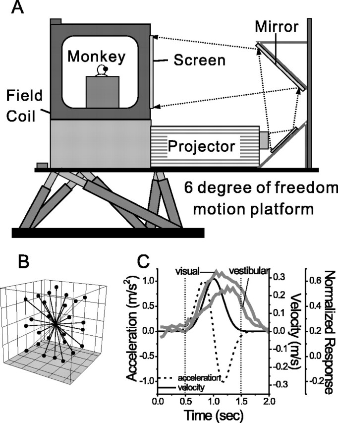
Experimental setup and heading stimuli. A, Schematic illustration of the virtualreality apparatus. The monkey, eye-movement monitoring system (field coil), and projector sit on top of a motion platform with six degrees of freedom. B, Illustration of the 26 movement vectors used to measure 3D heading tuning curves. C, Normalized population responses to visual and vestibular stimuli (gray curves) are superimposed on the stimulus velocity and acceleration profiles (solid and dashed black lines). The dotted vertical lines illustrate the 1 s analysis interval used to calculate mean firing rates.

A three-chip digital light projector (Christie Digital Mirage 2000; Christie, Cyrus, CA) was mounted on top of the motion platform to rear-project images onto a 60 × 60 cm tangent screen that was viewed by the monkey from a distance of 30 cm (thus subtending 90 × 90° of visual angle) (Fig. 1 A). This projector incorporates special circuitry such that image updating is precisely time locked to the vertical refresh of the video input (with a one-frame delay). The tangent screen was mounted on the front of the field coil frame. The sides, top, and back of the coil frame were covered with black enclosures such that the monkey's field of view was restricted to visual stimuli presented on the screen. The visual display, with a pixel resolution of 1280 × 1024 and 32-bit color depth, was updated at the same rate as the movement trajectory (60 Hz). Visual stimuli were generated by an OpenGL accelerator board (nVidia Quadro FX3000G; PNY Technologies, Parsippany, NJ), which was housed in a dedicated dual-processor personal computer. Visual stimuli were plotted with subpixel accuracy using hardware anti-aliasing.

In these experiments, visual stimuli depicted movement of the observer through a 3D cloud of “stars” that occupied a virtual space 100 cm wide, 100 cm tall, and 40 cm deep. Star density was 0.01/cm³, with each star being a 0.15 × 0.15 cm yellow triangle. Approximately 1500 stars were visible at any time within the field of view of the screen. Accurate rendering of the optic flow, motion parallax, and size cues that accompanied translation of the monkey was achieved by plotting the star field in a 3D virtual workspace and by moving the OpenGL “camera” through this space along the exact trajectory followed by the monkey's head. All visual stimuli were presented dichoptically at zero disparity (i.e., there were no stereo cues). The display screen was located in the center of the star field before stimulus onset and remained well within the depth of the star field throughout the motion trajectory. To avoid extremely large (near) stars from appearing in the display, a near clipping plane was imposed such that stimulus elements within 5 cm of the eyes were not rendered.

Platform motion and optic flow stimuli could be presented either together or separately (see below, Experimental protocol). During simultaneous presentation, stimuli were synchronized by eliminating time lags between platform motion and updating of the visual display using predictive control. In our apparatus, feedback from the motion platform actuators has a one-frame delay (16.7 ms), and there is an additional one-frame delay in the output of the projector. Thus, if we simply used feedback to directly update the visual display, there would be at least a 30–40 ms lag between platform motion and visual motion. To overcome this problem, we performed a dynamical systems analysis of the motion platform and constructed a transfer function that could be used to accurately predict platform motion from the command signal for a desired trajectory. We then time shifted the predicted position of the platform such that visual motion was synchronous with platform motion (to within ∼1 ms). To fine-tune the synchronization of visual and inertial motion stimuli, a world-fixed laser projected a small spot on the tangent screen, and images of a world-fixed crosshair were also rendered on the screen by the video card. While the platform was moved, a delay parameter in the software was adjusted carefully (1 ms resolution) until the laser spot and the crosshair moved precisely together. This synchronization was verified occasionally during the period of data collection.

To evaluate the accuracy of predictions from the transfer function, we input low-pass-filtered Gaussian white noise (20 dB cutoff at 4 Hz) as the command signal, and we compared the measured feedback signal (from the actuators) to the predicted position of the platform. We quantified the deviation of the prediction by computing the normalized root mean square (RMS) error between predicted and actual motion:

(1)

where P_f is measured feedback position, and Pp is the position predicted by the transfer function. The result of Equation 1 estimates the error relative to the signal. The normalized error was 0.038 for our noise input, indicating a close match between measured and predicted position of the platform (correlation coefficient, 0.998; p ≪ 0.001; n = 361 samples at 60 Hz). Thus, our dynamic characterization of the motion platform allowed highly synchronous and accurate combinations of visual and inertial motion to be presented.

Electrophysiological recordings. We recorded extracellularly the activities of single neurons from three hemispheres in two monkeys. A tungsten microelectrode (Frederick Haer Company, Bowdoinham, ME; tip diameter 3 μm, impedance 1–2 MΩ at 1 kHz) was advanced into the cortex through a transdural guide tube, using a micromanipulator (Frederick Haer Company) mounted on top of the Delrin ring. Single neurons were isolated using a conventional amplifier, a bandpass eight-pole filter (400–5000 Hz), and a dual voltage–time window discriminator (Bak Electronics, Mount Airy, MD). The times of occurrence of action potentials and all behavioral events were recorded with 1 ms resolution by the data acquisition computer. Eye movement traces were low-pass filtered and sampled at 250 Hz. Raw neural signals were also digitized at 25 kHz and stored to disk for off-line spike sorting and additional analyses.

Area MSTd was first identified using magnetic resonance imaging (MRI) scans. An initial scan was performed on each monkey before any surgeries using a high-resolution sagittal magnetization-prepared rapid-acquisition gradient echo sequence (0.75 × 0.75 × 0.75 mm voxels). SUREFIT software (Van Essen et al., 2001) was used to segment gray matter from white matter. A second scan was performed after the head holder and recording grid had been surgically implanted. Small cannulas filled with a contrast agent (Gadoversetamide) were inserted into the recording grid during the second scan to register electrode penetrations with the MRI volume. The MRI data were converted to a flat map using CARET software (Van Essen et al., 2001), and the flat map was morphed to match a standard macaque atlas. The data were then refolded and transferred onto the original MRI volume. Thus, MRI images were obtained showing the functional boundaries between different cortical areas, along with the expected trajectories of electrode penetrations through the guide tubes. Area MSTd was identified as a region centered ∼15 mm lateral to the midline and ∼3–6 mm posterior to the interaural plane.

Several other criteria were applied to identify MSTd neurons during recording experiments. First, the patterns of gray and white matter transitions along electrode penetrations were identified. MSTd was usually the first gray matter encountered that modulated its responses to flashing visual stimuli. Second, we mapped the receptive fields (RFs) of the MSTd neurons manually by moving a patch of drifting random dots around the visual field and observing a qualitative map of instantaneous firing rates on a custom graphical interface. MSTd neurons typically had large RFs that occupied a quadrant or a hemifield on the display screen. In most cases, RFs were centered in the contralateral visual field but also extended into the ipsilateral field and included the fovea. Many of the RFs were well contained within the boundaries of our display screen, but some RFs clearly extended beyond the boundaries of the screen. The average RF size was 44 ± 8 × 58 ± 13° SE, which is similar to RF sizes reported previously for MSTd (Van Essen et al., 1981; Desimone and Ungerleider, 1986; Komatsu and Wurtz, 1988a). Moreover, MSTd neurons usually were activated only by large visual stimuli (random-dot patches >10 × 10°), with smaller patches typically evoking little response. These properties are typical of neurons in area MSTd and distinct from the lateral subdivision of area MST (Komatsu and Wurtz, 1988a,b; Tanaka et al., 1993).

To further aid identification of recording locations, electrodes were often further advanced into the middle temporal area (area MT). There was usually a quiet region 0.3–1 mm long before MT was reached, which helped confirm the localization of MSTd. MT neurons were identified according to several properties, including smaller receptive fields (diameter ≈= eccentricity), sensitivity to small visual stimuli as well as large stimuli, and similar direction preferences within penetrations approximately normal to the cortical layers (Albright et al., 1984). The changes in receptive field location of MT neurons across guide tube locations were as expected from the known topography of MT (Zeki, 1974; Gattass and Gross, 1981; Van Essen et al., 1981; Desimone and Ungerleider, 1986; Albright and Desimone, 1987; Maunsell and Van Essen, 1987). Thus, we took advantage of the retinotopic organization of MT receptive fields to help identify the locations of our electrodes within MSTd (as described in Fig. 3).

Figure 3.

Summary of heading tuning in response to inertial motion in the vestibular condition versus complete darkness. A, Distribution of the differences in preferred heading for 14 neurons tested under the standard vestibular condition, with a fixation target, and in complete darkness with no requirement to fixate. The difference in preferred heading was binned according to the cosine of the angle (in accordance with the spherical nature of the data) (Snyder, 1987). B, Scatter plot of HTI values for the same 14 cells tested under both conditions. C, Scatter plot of the maximum response amplitude (R_max) under both conditions.

Experimental protocol. Once action potentials from a single MSTd neuron were satisfactorily isolated, the RF was mapped as described above. Next, regardless of the strength of visual responses, we tested the 3D heading tuning of the neuron by recording neural activity to heading stimuli presented along 26 heading directions corresponding to all combinations of azimuth and elevation angles in increments of 45° (Fig. 1 B). The stimuli were presented for a duration of 2 s, although most of the movement occurred within the middle 1 s. The stimulus trajectory had a Gaussian velocity profile and a corresponding biphasic acceleration profile. The motion amplitude was 13 cm (total displacement), with a peak acceleration of ∼0.1 g (∼0.98 m/s²) and a peak velocity of ∼30 cm/s (Fig. 1C). For inertial motion, these accelerations far exceed vestibular thresholds (for review, see Gundry, 1978) (Benson et al., 1986; Kingma, 2005).

The experimental protocol included three primary stimulus conditions. (1) In the “vestibular” condition, the monkey was moved along each of the 26 heading trajectories in the absence of optic flow. The screen was blank, except for a head-centered fixation point. Note that that we refer to this as the vestibular condition for simplicity, although other extraretinal signal contributions (e.g., from body proprioception) cannot be excluded. (2) In the “visual” condition, the motion platform was stationary while optic flow simulating movement through the cloud of stars was presented on the screen. (3) In the “combined” condition, the animal was moved using the motion platform while a congruent optic flow stimulus was presented. To measure the spontaneous activity of each neuron, additional trials without platform motion or optic flow were interleaved, resulting in a total of 395 trials (including five repetitions of each distinct stimulus). During all three cue conditions, the animal was required to fixate a central target (0.2° in diameter), which was introduced first in each trial and had to be fixated for 200 ms before stimulus onset (fixation windows spanned 1.5 × 1.5° of visual angle). The animals were rewarded at the end of each trial for maintaining fixation throughout stimulus presentation. If fixation was broken at any time during the stimulus, the trial was aborted and the data were discarded. Neurons were included in the sample if each stimulus was successfully repeated at least three times. Across our sample of MSTd neurons, 85% of cells were isolated long enough for at least five stimulus repetitions.

In some experiments, binocular eye movements were monitored to evaluate possible changes in vergence angle during stimulus presentation. Vergence angle was computed as the average difference in position of the two eyes over the middle 1 s interval of the Gaussian velocity profile. Because changes in vergence angle can be elicited by radial optic flow under some circumstances (Busettini et al., 1997), we examined how vergence angle depended on heading direction within the horizontal place (eight azimuth angles, 45° apart). We found no significant dependence of vergence angle on heading direction in any of the three stimulus conditions (one-way ANOVA, p > 0.05) (supplemental Fig. 1, available at www.jneurosci.org as supplemental material).

For a subpopulation of MSTd neurons that showed significant tuning in the vestibular condition, neural responses were also collected during platform motion along each of the 26 different directions in complete darkness (with the projector turned off). In these controls, there was no behavioral requirement to fixate and rewards were delivered manually to keep the animal motivated.

Data analysis. Because the responses of MSTd neurons primarily followed stimulus velocity (Fig. 1C), mean firing rates were computed during the middle 1 s interval of each stimulus presentation. When longer-duration analyses were used (i.e., 1.5 or 2 s), results were very similar. To quantify the strength of heading tuning for each of the vestibular, visual, and combined conditions, the mean firing rate in each trial was considered to represent the magnitude of a 3D vector whose direction was defined by the azimuth and elevation angles of the respective movement trajectory. A heading tuning index (HTI) was then computed as the magnitude of the vector sum of these individual response vectors, normalized by the sum of the magnitudes of the individual response vectors, according to the following equation:

(2)

where R_i is the mean firing rate for the ith stimulus direction after subtraction of spontaneous activity, and n corresponds to the number of different heading directions tested. The HTI ranges from 0 to 1 (weak to strong tuning). Its statistical significance was assessed using a permutation test based on 1000 random reshufflings of the stimulus directions. The preferred heading direction for each stimulus condition was computed from the azimuth and elevation of the vector sum of the individual responses (numerator of Eq. 2).

Our heading tuning functions are intrinsically spherical in nature because we have sampled heading directions uniformly around the sphere (Fig. 1 B). To plot these spherical data on Cartesian axes (see Fig. 2), we have transformed the data using the Lambert cylindrical equal-area projection (Snyder, 1987). In these flattened representations of the data, the abscissa represents the azimuth angle, and the ordinate represents a sinusoidally transformed version of the elevation angle.

Figure 2.

Examples of 3D heading tuning functions for three MSTd neurons. Color contour maps show the mean firing rate as a function of azimuth and elevation angles. Each contour map shows the Lambert cylindrical equal-area projection of the original spherical data (see Materials and Methods) (Snyder, 1987). In this projection, the ordinate is a sinusoidally transformed version of elevation angle. Tuning curves along the margins of each color map illustrate mean ± SEM firing rates plotted as a function of either elevation or azimuth (averaged across azimuth or elevation, respectively). Data from the vestibular, visual, and combined stimulus conditions are shown from left to right. A, Data from a neuron with congruent tuning for heading defined by visual and vestibular cues. B, Data from a neuron with opposite heading preferences for visual and vestibular stimuli. C, Data from a neuron with strong tuning for heading defined by optic flow but no vestibular tuning. D, Definitions of azimuth and elevation angles used to define heading stimuli in 3D.

Mathematical description of heading tuning functions. To simulate the behavior of a network of units that resemble MSTd neurons, it was first necessary to obtain a simple mathematical model that could adequately describe the heading selectivity of MSTd cells. After evaluating several alternatives, we found that the 3D heading tuning of MSTd neurons could be well described by a modified sinusoid function (MSF) having five free parameters:

(3)

where R is the response amplitude, azi is the azimuth angle (range, 0–2π), and ele is the elevation angle (range, –π /2 to π /2). The azi and ele variables in Equation 3 have been expressed in rotated spherical coordinates such that the peak of the function, given by parameters (azi_p, ele_p), lies at the preferred heading of the neuron in 3D. Thus, the five free parameters are the preferred azimuth (azi_p), the preferred elevation (ele_p), response modulation amplitude (A), the baseline firing rate (DC), and the exponent parameter (n) of the nonlinearity G. The nonlinear transformation G() is given by the following:

(4)

where n (constrained to be >0) is the parameter that controls the nonlinearity. When n is close to zero, G(x) has no effect on the tuning curve. As n gets larger, this function amplifies and narrows the peak of the tuning function, while suppressing and broadening the trough. The operation []* in Equation 3 represents normalization to the range [–1,1] after application of the nonlinearity. This normalization avoids confounding the nonlinearity parameter, n, with the amplitude and DC offset parameters. Goodness of fit was quantified by correlating the mean responses of neurons with the model fits (across heading directions).

Network model: design and training. A simple feedforward two-layer artificial neural network was implemented, trained using backpropagation, and used to explore intermediate representations of visual and vestibular signals that might contribute to heading perception. The MSF described by Equation 3 was used to characterize the heading tuning of input and output units in the model. The nonlinearity (n), amplitude (A), and DC response parameters in the MSF were set to 1, 1.462, and –0.462, respectively, so that the responses of input and output units were normalized to the range of [–1,1]. These values were chosen because they produced tuning functions similar to the majority of MSTd neurons. Hidden layer units in the network were characterized by hyperbolic tangent (sigmoid) activation functions, whereas the output layer units had linear activation functions. The network was fully connected, such that each hidden layer unit was connected to all inputs and each output unit was connected to all hidden layer units. It can be shown that such a network is capable of estimating an arbitrary function, given a sufficient number of hidden units (Bishop, 1995).

The network had 26 visual input units, each with a different heading preference around the sphere (spaced apart as in Fig. 1 B). The 26 vestibular input units and 26 output units also had heading preferences spaced uniformly on the sphere. Visual input units coded heading in an eye-centered spatial reference frame, whereas vestibular input units and output units coded heading in a head-centered reference frame. The overall heading estimate of the network, resulting from the activity of the output units, was defined by a population vector (Georgopoulos et al., 1986) and was computed as the vector sum of the responses of the 26 output units. The network also received 12 eye-position inputs, each with a response that was a linear function of eye position. Six units coded horizontal eye position (three different positive slopes and three different negative slopes), and six units coded vertical eye positions (with the same slopes).

The network was trained to compute the correct direction of heading, in a head-centered reference frame, under each of the simulated vestibular, visual, and combined conditions. For all combinations of heading directions and eye positions, network connection weights were adjusted to minimize the sum squared error between the actual outputs of the network and the desired outputs, plus the sum of the absolute values of all network weights and biases. The second term caused training to prefer networks with the smallest set of weights and biases. The network was built and trained using the Matlab Neural Network Toolbox (Math-Works, Natick, MA), with the basic results being independent of the particular minimization algorithm used. The data presented here were obtained using the scaled conjugate gradient algorithm, which typically provided the best performance. When analyzing the responses of model units (see Figs. 10, 11, 12), to avoid unrealistic negative response values, we subtracted the minimum response of each unit to make all responses positive.

Figure 10.

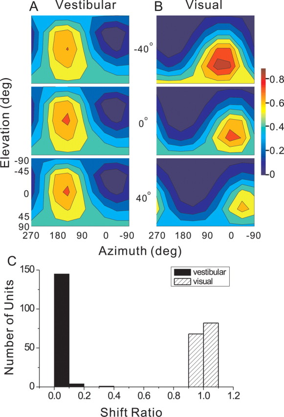
A, B, Example of 3D heading tuning functions for a network hidden unit tested at three horizontal eye positions (from top to bottom, 40° left, 0°, and 40° right) under the vestibular (A) and visual (B) conditions. The format is similar to Figure 2. C, Shift ratio distributions for all 150 hidden units under the two single-cue conditions.

Figure 11.

Comparison of heading selectivity for hidden layer units across different conditions. Scatter plots of HTI for the visual versus vestibular conditions (A), the combined versus vestibular conditions (B), and the combined versus visual conditions (C). The format is the same as in Figure 6A–C. D, Average ± SEM results from five training sessions. Filled circles, Visual versus vestibular; open circles, combined versus vestibular; triangles, combined versus visual conditions. The stars illustrate the means corresponding to the data in A–C. The lines illustrate the diagonals (unity slope).

Figure 12.

Distribution of the absolute difference in preferred heading, |Δ Preferred Heading|, for the hidden layer units between the visual and vestibular conditions (A), the combined and vestibular conditions (B), and the combined and visual conditions (C). Data are means ± SD from five training sessions. The format is the same as in Figure 6D–F.

In each simulated stimulus condition, horizontal/vertical eye position took on one of five possible values from trial to trial: ±40, ±20, and 0°. In the simulated visual condition, the network was only given visual inputs and eye-position inputs and was trained to compute heading direction in a head-centered frame of reference. Thus, in this condition, the network was required to interact eye-position signals with visual inputs, because the latter originated in an eye-centered reference frame. In the simulated vestibular condition, although input signals were already in a head-centered reference frame, the network was again given both vestibular and eye-position inputs. In the simulated combined condition, all inputs were active and the network was again required to compute heading direction in a head-centered reference frame. Thus, across all stimulus conditions and eye positions, the network was required to selectively transform visual inputs from eye centered to head centered, while retaining correct behavior for vestibular inputs. Whereas the reference frames used by the input units were fixed (by design), hidden units in the model could potentially code heading in any reference frame. The reference frames of hidden units were quantified by computing a “shift ratio,” which was defined as the observed change in heading preference between a pair of eye positions divided by the difference in eye position. Shift ratios near 0 indicate a head-centered reference frame, and values near 1 represent an eye-centered reference frame.

Results

The activities of 255 MSTd neurons from two monkeys (169 from monkey 1 and 86 from monkey 2) were characterized during actual and simulated motions along a variety of different headings in 3D space, using a virtual-reality apparatus (Fig. 1A). We recorded from every well isolated neuron in MSTd that was spontaneously active or that responded to a large flickering field of random dots. MSTd was localized based on multiple criteria, as described in Materials and Methods. Every MSTd neuron was tested under three stimulus conditions in which heading direction was defined by inertial motion alone (vestibular condition), optic flow alone (visual condition), or congruent combinations of inertial and visual motion (combined condition). Note that heading directions in all conditions are referenced to physical body motion (i.e., heading direction for optic flow refers to the direction of simulated body motion).

To quantify heading selectivity in the following analyses, the mean neural firing rate for each heading was calculated from the middle 1 s of the stimulus profile (see Materials and Methods), a period that contains most of the velocity variation. As illustrated in Figure 1C, the population responses to either optic flow or inertial motion look much more like delayed and smeared out versions of stimulus velocity than stimulus acceleration (Fig. 1C, compare population responses with black solid and dashed lines). Each population response was computed as a peristimulus time histogram (PSTH), by summing up the contribution of each cell, which was taken along the heading direction that produced the maximum response, with each 50 ms bin being normalized by the maximum bin. The dynamics of MSTd responses were further analyzed by computing correlation coefficients between the PSTH of each neuron and the velocity and acceleration profiles of the stimulus, using a range of correlation delays from 0 to 300 ms. For >90% of neurons in each stimulus condition, the maximum correlation with velocity was larger than that for acceleration (paired t test, p ≪ 0.001).

The responses of the majority of MSTd neurons were modulated by heading direction under all three stimulus conditions. Figure 2 shows typical examples of heading tuning in MSTd, illustrated as contour maps of mean firing rate (represented by color) plotted as a function of azimuth (abscissa) and elevation (ordinate). The MSTd cell illustrated in Figure 2A represents a “congruent” neuron, for which heading tuning is quite similar for visual and vestibular inputs. The cell exhibited broad, approximately sinusoidal tuning, with a peak response during inertial motion at 0° azimuth and –30° elevation, corresponding to a rightward and slightly upward trajectory (vestibular condition, left column). A similar preference was observed under the visual condition (middle column), with the peak response occurring for simulated rightward/upward trajectories. As expected based on the congruent tuning of this neuron for visual and vestibular stimuli, a similar heading preference was also seen in the combined condition (Fig. 2A, right column). However, the peak response in the combined condition was not strengthened compared with the visual condition, suggesting that sensory information might not be linearly combined in the activities of MSTd neurons.

Congruent cells such as this one might be useful for coding heading under natural conditions in which both inertial and optic flow cues provide information about self-motion. However, many MSTd neurons were characterized by opposite tuning preferences in the visual and vestibular conditions. Figure 2B shows an example of an “anti-congruent” cell, with a preferred heading for the vestibular condition that was nearly opposite to that in the visual condition. Both the heading preference and the maximum response in the combined condition were similar to those in the visual condition, suggesting that vestibular cues were strongly deemphasized in the combined response. A third main type of neuron encountered in MSTd, with heading-selective responses only in the visual and combined conditions but not the vestibular condition, is illustrated in Figure 2C.

In the following, we first summarize heading tuning properties under each single-cue condition. We then examine closely the relationship between heading tuning in the combined condition and that in the single-cue conditions.

Single-cue responses

The strength of heading tuning of MSTd neurons was quantified using a HTI, which ranges from 0 to 1 (poor and strong tuning, respectively; see Materials and Methods). For reference, a neuron with idealized cosine tuning would have an HTI value of 0.31, whereas an HTI value of 1 is reached when firing rate is zero (spontaneous) for all but a single stimulus direction. For the visual condition, HTI values averaged 0.48 ± 0.16 SD, with all but four cells (251 of 255, 98%) being significantly tuned, as assessed by a permutation test (p < 0.05). For the vestibular condition, HTI values were generally smaller (mean ± SD, 0.26 ± 0.16), with only 64% of neurons (162 of 255) being significantly tuned (p < 0.05). Across the population, the HTI for the vestibular condition was significantly smaller than that for the visual condition (paired t test, p ≪ 0.001).

Because of the behavioral requirement to maintain fixation on a head-fixed central target, significant heading tuning under the vestibular condition might not necessarily represent sensory responses to inertial motion. For example, the observed responses could be driven by a pursuit-like signal related to suppression of the vestibulo-ocular reflex (VOR) (Thier and Erickson, 1992a,b; Fukushima et al., 2000). To examine this possibility, 14 neurons were also tested using a modified vestibular condition, in which the animal sat in complete darkness and there was no requirement to maintain fixation. We found that heading tuning in complete darkness was very similar to that seen during the standard fixation task. First, the absolute difference in heading preference between these two conditions was small, with a mean value of 17.4 ± 9.9° SD (Fig. 3A). In addition, neither the HTI (paired t test, p = 0.54) nor the maximum response (paired t test, p = 0.18) was significantly different between the two conditions (Fig. 3B,C). These results suggest that heading tuning in the vestibular condition reflects sensory signals that arise from vestibular and/or proprioceptive inputs rather than a VOR suppression or pursuit-like signal (see Discussion).

Neurons with significant vestibular tuning were not uniformly distributed within MSTd. Across animals, there was a significant (ANOVA, p ≪ 0.001) difference between vestibular HTI values for the three hemispheres, with means ± SEM of 0.20 ± 0.01, 0.26 ± 0.02, and 0.33 ± 0.05 for the left hemisphere of monkey 1, the right hemisphere of monkey 1, and the right hemisphere of monkey 2, respectively. No significant difference between hemispheres was found for visual HTI values (ANOVA, p = 0.42). At most guide tube locations, we advanced the electrodes past MSTd and mapped RFs in area MT. HTI values for the vestibular condition have been plotted against the polar angle of the underlying MT RFs in Figure 4. For the two right hemispheres, which also had the largest average HTI values, there was a significant dependence of HTI on MT receptive field location (correlation coefficient, r =–0.4; p ≪ 0.001), with larger HTI values for MT RFs in the lower hemifield (Fig. 4, filled symbols). The solid line through the data points is the running median, computed using 30° bins at a resolution of 5°. Based on the known topography of MT (Zeki, 1974; Gattass and Gross, 1981; Van Essen et al., 1981; Desimone and Ungerleider, 1986; Albright and Desimone, 1987; Maunsell and Van Essen, 1987), this relationship suggests that vestibular tuning tends to be stronger in the posterior medial portions of MSTd. No such relationship was found for the left hemisphere of monkey 1 (Fig. 4, open symbols and gray line) (correlation coefficient, r =–0.13; p = 0.5). These results suggest that a gradient of vestibular heading selectivity might exist within area MSTd.

Figure 4.

Relationship between the HTI for the vestibular condition and recording location within MSTd. Recording location was estimated from the polar angle of the underlying MT receptive field, with 90°/–90° corresponding to the upper/lower vertical meridian and 0° to the horizontal meridian in the contralateral visual field. Thus, moving from left to right along the abscissa corresponds approximately to moving from posteromedial (PM) to anterolateral (AL) within MSTd. The thick lines through the data illustrate the running median, using a bin width of 30° and a resolution of 5°. Data are shown separately for the right (filled symbols and black line; n = 153) and left (open symbols and gray line; n = 62) hemispheres.

For cells with significant tuning (p < 0.05, permutation test), the heading preference was defined as the azimuth and elevation of the vector average of the neural responses (see Materials and Methods). Heading preferences in MSTd were distributed throughout the spherical stimulus space, but there was a significant predominance of cells that preferred lateral versus fore-aft motion directions in both single-cue conditions (Fig. 5). For both the visual and vestibular conditions, the distribution of preferred azimuths was significantly bimodal, with peaks at ∼0 and 180°, respectively [Fisher's test for uniformity against a bipolar alternative, p < 0.01) (Fisher et al., 1987)].

Figure 5.

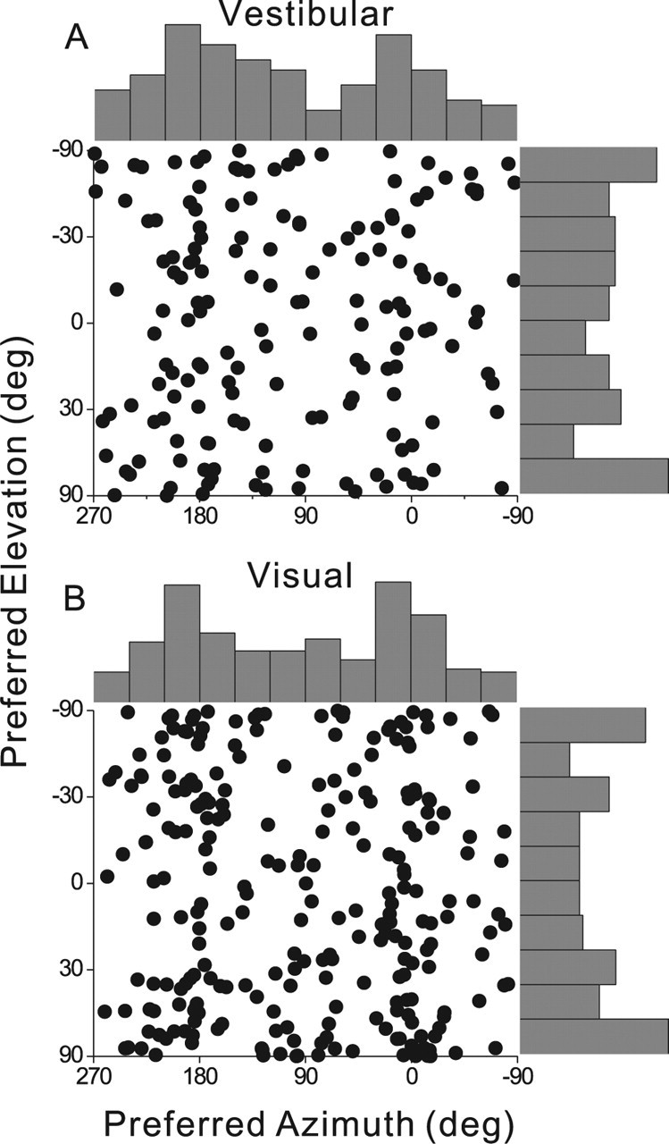
Distributions of 3D heading preferences of MSTd neurons for the vestibular condition (A) and the visual condition (B). Each data point in the scatter plot corresponds to the preferred azimuth (abscissa) and elevation (ordinate) of a single neuron with significant heading tuning (A, n = 162; B, n = 251). The data are plotted on Cartesian axes that represent the Lambert cylindrical equal-area projection of the spherical stimulus space. Histograms along the top and right sides of each scatter plot show the marginal distributions.

Relationship between visual/vestibular tuning and combined cue responses

If MSTd neurons integrate vestibular and visual signals to achieve better heading selectivity, the combination of the two cues should produce stronger heading tuning than either single cue alone. Scatter plots of HTI for all paired combinations of the visual, vestibular, and combined conditions are illustrated in Figure 6A–C. A bootstrap analysis revealed that the visual HTI was significantly larger (p < 0.05) than the vestibular HTI for 62% (157 of 255) of MSTd neurons (Fig. 6A, filled symbols above the diagonal). The reverse was true for only 5% (14 of 255) of neurons (Fig. 6A, filled symbols below the diagonal). Similarly, for 57% (144 of 255) of the cells, the combined condition also resulted in larger HTI values compared with the vestibular condition (Fig. 6B, filled symbols above the diagonal). The reverse was true for only 10% (25 of 255) of the cells (Fig. 6B, filled symbols below the diagonal).

Figure 6.

Comparison of heading selectivity (A–C) and tuning preferences (D–F) of MSTd neurons across stimulus conditions. A, The HTI for the visual condition plotted against the HTI for the vestibular condition. B, HTI for the combined condition versus HTI for the vestibular condition. C, HTI for the combined condition versus HTI for the visual condition. Filled and open circles, Cells with and without significantly different HTI values for the two conditions, respectively (bootstrap; n = 1000; p < 0.05). n = 255 cells. The solid lines indicate the unity-slope diagonal. D–F, Distribution of the difference in preferred heading, Δ Preferred Heading, between the following: D, the visual and vestibular conditions (n = 160); E, the combined versus vestibular conditions (n=156); F, the combined versus visual conditions (n = 239). Note that bins were computed according to the cosine of the angle (in accordance with the spherical nature of the data) (Snyder, 1987). Only neurons with significant heading tuning in each pair of conditions have been included.

Although adding optic flow to inertial motion generally improved spatial tuning (paired t test, p ≪ 0.001), the converse was not true. Instead, adding inertial motion to optic flow actually reduced heading selectivity, such that the average HTI for the combined condition was lower than that in the visual condition (paired t test, p ≪ 0.001). This is illustrated in Figure 6C, in which 36% (93 of 255) of the neurons had a combined HTI that was significantly smaller than the visual HTI (filled symbols below the diagonal). For only 7% (19 of 255) of the neurons did the combination of cues result in a higher HTI than the optic flow stimulus alone (Fig. 6C, filled symbols above the diagonal). For the remaining 57% of the cells, the tuning indices for the combined and visual conditions were not significantly different (Fig. 6C, open symbols). Thus, combining visual and nonvisual cues generally did not strengthen, but frequently weakened, the tuning of MSTd neurons to optic flow.

The lack of improvement in HTI under the combined condition is at least partly attributable to the fact that many MSTd neurons did not have congruent heading preferences in the visual and vestibular conditions (Fig. 2B). The distributions of the absolute differences in preferred heading (|Δ Preferred Heading|) between the three stimulus conditions are summarized in Figure 6D–F for all neurons with significant heading tuning. This metric is the smallest angle between a pair of preferred heading vectors in 3D. Note that |Δ Preferred Heading| is not plotted on a linear axis because of the spherical nature of the data. If the preferred heading vectors for the visual and vestibular conditions were distributed randomly around the sphere, then |Δ Preferred Heading| would not be distributed uniformly on a linear scale but would rather have a clear peak at ∼90°. Instead, the |Δ Preferred Heading| values have been transformed sinusoidally such that the distribution would be flat if the preferred heading vectors for visual and vestibular conditions were not correlated.

The distribution of |Δ Preferred Heading| between the visual and vestibular conditions was broad and clearly bimodal [Silverman's bimodal test, p < 0.001 (Silverman, 1986)], indicating that visual and vestibular heading preferences tended to be either matched or opposite (Fig. 6D). The distribution of |Δ Preferred Heading| between the combined and vestibular conditions was also very broad and significantly bimodal (Fig. 6E), indicating that the vestibular heading preference was often not a good predictor of the combined preference. In contrast, the difference in heading preference between the combined and visual conditions showed a very narrow distribution centered close to 0° (Fig. 6F). Therefore, the heading preference in the combined condition was strongly dominated by the tuning for optic flow.

Poorly matched heading preferences between the visual and vestibular conditions (Fig. 6D) may explain the weakened heading tuning in the combined condition relative to visual when both cues were provided (Fig. 6C). Indeed, when the difference in HTI between the combined and visual conditions was plotted against |Δ Preferred Heading| for the visual and vestibular conditions, a significant trend (Spearman's rank correlation, r =–0.35; p ≪ 0.001) was observed (Fig. 7). The larger the |Δ Preferred Heading| between the visual and vestibular conditions, the smaller the HTI for the combined relative to the visual condition. However, even for congruent visual and vestibular heading preferences (gray area), heading selectivity was not significantly strengthened in the combined condition overall (mean ± SD HTI difference, –0.02 ± 0.01; p = 0.23). Therefore, poor matching of the visual and vestibular heading preferences only partially explains the weakened tuning in the combined condition.

Figure 7.

Scatter plot of the difference in HTI between the combined and visual conditions plotted against the difference in preferred heading, |Δ Preferred Heading|, between the vestibular and visual conditions. Filled and open symbols, Cells with and without significantly different HTI values for the combined and visual conditions, respectively (bootstrap; n = 1000; p<0.05; from Fig. 6C). Solid line, Best linear fit through all data (both open and filled symbols). Gray area highlights neurons with vestibular and visual heading preferences matched to within 45°. Only neurons with significant tuning in both the vestibular and visual conditions are included (n = 160).

To further explore the vestibular contribution to combined cue responses, we estimated a “vestibular gain,” defined as the fraction of the vestibular responses of a cell that must be added to the visual responses to explain the combined tuning. This can be described as follows:

(5)

where R_x are matrices of mean firing rates for all heading directions, a is the vestibular gain, and b is a constant that can account for direction-independent differences between the three conditions. If a = 1, vestibular and visual modulations contribute to the combined response in proportion to the strengths of the individual cue responses. In contrast, when a = 0, vestibular responses make no contribution, such that the combined response is determined exclusively by the visual modulation. For values of a between 0 and 1, vestibular signals contribute less than expected from responses to the single-cue conditions, whereas the reverse is true for values of a larger than 1. The vestibular gain for MSTd neurons with significant vestibular tuning averaged 0.30 ± 0.45 SD and was significantly different from both 0 and 1 (t test, p ≪ 0.001). Only a weak correlation existed between vestibular gain and the ratio of the vestibular and visual HTIs (Fig. 8) (linear regression, r = 0.19; p = 0.002), such that even neurons with strong vestibular tuning typically had vestibular gains <0.5. Thus, the vestibular signal contribution appeared to be consistently deemphasized in the combined condition.

Figure 8.

Quantification of vestibular contribution to the combined response. The vestibular gain, a (Eq. 5), for all 255 MSTd neurons is plotted as a function of the ratio between HTI values for the vestibular and visual conditions. Filled and open symbols denote neurons with and without significant vestibular tuning, respectively. Solid line, Linear regression through all data points.

In summary, these results illustrate that, although the majority of MSTd neurons were significantly tuned for heading in response to both optic flow and inertial motion, heading preferences were poorly matched and responses to the combined stimulus were dominated by the visual responses of the cell. Importantly, adding nonvisual motion-related signals to the visual responses generally did not improve heading selectivity but actually weakened spatial tuning.

Model predictions/simulations

The experimental observations described above appear to be inconsistent with the hypothesis that MSTd neurons have integrated visual and nonvisual cues for heading perception. So how might we explain the vestibular heading tuning of MSTd neurons? Related to the potential role of MSTd in sensory integration is the fact that optic flow and vestibular signals are known to originate in different spatial reference frames. Specifically, visual motion signals originate in retinal coordinates (Squatrito and Maioli, 1996, 1997; Bremmer et al., 1997), whereas vestibular signals are head/body centered (Shaikh et al., 2004). It is often assumed that optic flow signals must first be converted into a head-centered reference frame, before being useful for heading perception (Royden, 1994; Royden et al., 1994; Banks et al., 1996).

It is not immediately obvious what patterns of visual/vestibular interactions might be expected within a network that performs a reference-frame transformation selectively for one sensory cue (visual) versus another (vestibular). To explore potential visual/vestibular interactions that could emerge within cell populations that perform such a selective reference-frame transformation, we implemented a very simple two-layer neural network model (Fig. 9) that receives eye-centered visual inputs, head-centered vestibular inputs, and eye-position signals. The network was trained to compute the (head-centered) heading direction of the head/body in space regardless of whether this was specified by visual cues, vestibular cues, or both together. To simulate the responses of model neurons, we used a five-parameter MSF (see Eq. 3 in Materials and Methods) that was found to adequately describe the 3D heading tuning functions of MSTd neurons (average r² = 0.79 ± 0.02 SE and 0.88 ± 0.01 SE for the vestibular and visual conditions, respectively). Other technical details regarding the network model can be found in Materials and Methods.

Figure 9.

Schematic diagram of a simple two-layer, feedforward neural network model that was trained to compute the head-centered direction of heading from eye-centered visual inputs, head-centered vestibular inputs, and eye-position signals. Hidden units (n = 150) have sigmoidal activation functions, whereas output units are linear.

To provide an intuitive appreciation of the computations performed by the network, Figure 10, A and B, illustrates the 3D heading tuning of a typical hidden layer unit under the simulated vestibular and visual conditions, plotted separately for three eye positions: 0°, which corresponds to straight ahead (middle row), 40° left (top row), and 40° right (bottom row). Vestibular responses did not depend on eye position, indicating that heading was coded in a head-centered (or body-centered) reference frame (Fig. 10A). In contrast, the visual responses of this hidden unit shifted systematically with eye position, as expected for an eye-centered reference frame (Fig. 10B). This pattern was typical of all hidden units, as illustrated in Figure 10C, which summarizes the mean shift ratio of all hidden layer units under the vestibular and visual conditions (black and gray fills, respectively). The shift ratio was computed as the observed change in preferred heading between a pair of eye positions divided by the difference in eye position. Shift ratios near 0 represent coding of heading in a head-centered frame, whereas shift ratios near 1 correspond to an eye-centered reference frame. The shift ratio of 150 hidden units averaged 0.01 ± 0.04 SD for the vestibular condition and 1.0 ± 0.01 SD for the visual condition (Fig. 10C).

As demonstrated previously by Zipser and Andersen (1988), the transformation of optic flow signals from an eye-centered to head-centered reference frame was implemented in the hidden layer of our model through modulation of hidden unit responses by eye position (i.e., gain fields). This is illustrated for the example hidden unit in Figure 10B, in which larger responses were seen when eye position was 40° to the left than 40° to the right. This effect was quantified for all hidden layer units using linear regression. The absolute values of the regression slopes were approximately fourfold larger for the visual than the vestibular condition, and this difference in gain field strength was highly significant (paired t test, p ≪ 0.001). Thus, the network implemented the reference-frame transformation for optic flow through gain modulation, whereas vestibular signals remained essentially unaltered. Keeping this functionality of the network in mind, we next summarize the tuning strengths and heading preferences of hidden layer units in the network.

For a direct comparison between response properties of hidden layer units and MSTd neurons, we quantified hidden layer tuning using the same metrics described in the previous sections. HTI values for each pairing of visual, vestibular, and combined conditions are illustrated in Figure 11A–C. Each panel shows data from 150 hidden layer units obtained from one representative training session of the network. In agreement with the experimental observations, HTI values for hidden units in the vestibular condition (0.33 ± 0.007 SE) were significantly smaller than HTI values for the visual condition (0.37 ± 0.008 SE) (paired t test, p ≪ 0.001) (Fig. 11A). In addition, HTI values for the combined condition (0.36 ± 0.006 SE) were significantly larger than those for the vestibular condition (paired t test, p ≪ 0.001) (Fig. 11B) but marginally smaller than HTI values for the visual condition (paired t test, p = 0.025) (Fig. 11C). Mean HTI values were fairly consistent across different network training sessions (Fig. 11D) (ANOVA, p > 0.05), as were differences in HTIs among stimulus conditions. Thus, similar to the properties of MSTd neurons (Fig. 6), hidden units showed stronger heading tuning for the visual than the vestibular condition and slightly weaker heading selectivity for the combined condition relative to the visual condition. These differences in HTIs were substantially smaller for hidden units than for MSTd neurons, but the overall pattern of results was quite similar.

Importantly, there were also striking similarities between hidden layer units and MSTd neurons when considering the relationships between heading preferences across stimulus conditions. Figure 12 summarizes the mean ± SE of the |Δ Preferred Heading| values from five training sessions, in a format similar to that shown for MSTd neurons in Figure 6. There was little correlation between preferred headings for the vestibular and visual conditions (Fig. 12A), such that the distribution of |Δ Preferred Heading| was broad with a significant tendency toward bimodality [Silverman's bimodal test, p < 0.01 (Silverman, 1986)]. The distribution of |Δ Preferred Heading| between the combined and vestibular conditions, although clearly skewed more toward zero, was also quite broad (Fig. 12B). In contrast, the histogram of |Δ Preferred Heading| between the combined and visual conditions was more strongly skewed toward zero (t test, p ≪ 0.001) (Fig. 12C), similar to the MSTd data (Fig. 6F). Interestingly, when the network was trained to compute heading in an eye-centered reference frame under all three stimulus conditions, thus requiring a reference frame change for vestibular signals but not for visual signals, we found the opposite pattern of results (combined responses were dominated by the vestibular inputs). Thus, a simple network trained to perform a reference-frame transformation for only one of two sensory inputs predicts a hidden layer network whose responses are dominated by the transformed input and an inconsistent pattern of relative heading preferences for the two sensory cues. Considering that a reference frame change is necessary for visual (but not vestibular) cues to compute heading in head/body-centered coordinates, the properties of network hidden units qualitatively recapitulate the basic features of heading selectivity observed in area MSTd.

Discussion

Using a virtual-reality system to provide actual and/or simulated motion in 3D space, we have shown that, although the majority of MSTd neurons exhibited significant heading tuning in the vestibular condition, the addition of inertial motion to optic flow generally did not improve heading selectivity. Rather, heading tuning in the combined condition was dominated by optic flow responses and was typically weakened relative to the visual condition. In addition, heading preferences between the vestibular and visual conditions were often opposite. These findings were qualitatively predicted by the properties of hidden units in a simple neural network that received head-centered vestibular signals and eye-centered optic flow information. The network computed heading in a head-centered reference frame by transforming the visual, but not the vestibular, inputs. Hidden layer properties were biased toward the input that undergoes the transformation and resemble in many respects the properties of MSTd neurons.

Vestibular signals in MSTd

Spatial tuning driven by inertial motion has been described previously in MSTd (Duffy, 1998; Bremmer et al., 1999; Page and Duffy, 2003). The percentage of neurons with significant vestibular tuning in our experiments (64%) is substantially higher than that of previous studies (e.g., 24% in the study of Duffy, 1998). A likely explanation for these differences is our use of 3D motion and a Gaussian velocity profile that provides a more efficient linear acceleration stimulus to otolith afferents (Fernandez et al., 1972; Fernandez and Goldberg, 1976a,b). Recording location may also be a factor, because our analyses suggest that vestibular tuning is stronger in posteromedial portions of MSTd in the right hemisphere. Although our data do not allow us to make strong conclusions regarding hemispheric differences, they are consistent with findings of a right-hemispheric dominance of vestibular responses in functional MRI (fMRI) experiments involving caloric stimulation (Fasold et al., 2002).

Although we refer to our inertial motion stimulus as the vestibular condition, responses to this stimulus might not be exclusively vestibular in nature. There are at least two alternative possibilities regarding their origin. First, they might represent efference copy signals related to VOR cancellation. We have excluded this possibility by showing that responses of a subpopulation of MSTd neurons in the vestibular condition were nearly identical when tested in complete darkness without any requirement for fixation (Fig. 3). Second, MSTd responses during inertial motion in the absence of optic flow might also arise from skin receptors and body proprioceptors (for review, see Lackner and DiZio, 2005). Although we cannot exclude this possibility, a recent fMRI study has reported only visual and vestibular (but not proprioceptive) activation in area hMT/visual area 5 (V5) (Fasold et al., 2004).

Temporal dynamics of MSTd responses

One barrier to integrating vestibular and visual signals for heading perception is that these signals are initially encoded with different temporal dynamics. Inertial motion acceleration is encoded by primary otolith afferents (Fernandez and Goldberg, 1976). In contrast, visual motion is thought to be encoded in terms of velocity signals (Rodman and Albright, 1987; Lisberger and Movshon, 1999) (but see Cao et al., 2004). If MSTd neurons integrate vestibular and visual information, these signals should be coded with similar dynamics. Using stimuli with a Gaussian velocity profile has allowed us to demonstrate that the response dynamics of MSTd neurons, in both the vestibular and visual conditions, follow more closely the stimulus velocity profile rather than the biphasic acceleration profile (Fig. 1C). In contrast, previous MSTd studies have used constant velocity stimuli (Duffy, 1998; Page and Duffy, 2003), which have the disadvantage of not appropriately activating primary otolith afferents. Our results suggest that vestibular and visual responses in MSTd satisfy the temporal requirement of sensory integration.

At the population level, vestibular and visual responses extend considerably beyond the time course of the stimulus (Fig. 1C). This could be attributable to individual neurons having sustained responses or to latency variation across the population. A detailed analysis of response dynamics will be presented elsewhere, but we note here that both factors clearly contribute to the observed population responses.

Visual/vestibular interactions in MSTd

For neurons that integrate sensory cues for heading perception, a sensible expectation is that heading preferences should be matched for the two single-cue conditions and that heading tuning should be more robust under the combined condition. In contrast, we found that single-cue heading preferences were frequently opposite and that adding inertial motion cues to optic flow generally impaired heading selectivity. These findings extend previous work done in MSTd using 1D or 2D stimulation (Duffy, 1998; Bremmer et al., 1999). In an experiment involving 1D (fore-aft) motion on a parallel swing, Bremmer et al. (1999) reported that approximately half of MSTd neurons showed opposite heading preferences for visual and vestibular stimulation. In a 2D experiment involving constant-velocity motion in the horizontal plane, Duffy (1998) reported no correlation between heading preferences for visual and vestibular stimulation and described generally weaker heading selectivity under combined stimulation than visual stimulation. In addition to extending these previous studies to 3D, we have reported an additional relationship between heading strength and heading preference: larger differences in heading preference between single-cue conditions were correlated with weaker heading tuning in the combined condition relative to the visual condition (Fig. 7). These findings are consistent with some fMRI and positron emission tomography results, in which activation of area hMT/V5 was significantly smaller when optic flow was combined with caloric or electrical vestibular stimulation (Brandt et al., 1998, 2002). Thus, the available data suggest that MSTd neurons may not integrate visual and vestibular cues to allow more robust heading perception.

The reference-frame problem for heading perception

Vestibular and visual signals not only originate with different temporal dynamics but also encode motion in different spatial reference frames. Inertial motion signals, originating from the otolith organs of the inner ear, measure linear accelerations of the head, i.e., they reflect heading in head-centered coordinates. Conversely, visual motion signals originate in eye-centered coordinates and thus encode heading direction relative to the current position of the eyes. For visual and vestibular signals to interact synergistically for heading perception, they may need to be brought into a common spatial reference frame. This common frame could be eye centered, head centered, or an intermediate frame in which visual and vestibular signals are dependent on both head and eye position.

Although previous studies have shown that responses of some MST neurons are at least partially compensated for the velocity of eye and head movements (Bradley et al., 1996; Page and Duffy, 1999; Shenoy et al., 1999, 2002; Ilg et al., 2004), this does not necessarily indicate that MST codes motion in a head- or world-centered reference frame (i.e., velocity compensation does not necessarily imply position compensation). The reference frame for heading selectivity based on optic flow in MSTd has not yet been examined during static fixation at different eye positions, although MSTd receptive fields have been reported to be primarily eye centered with gain modulations (Squatrito and Maioli, 1996, 1997; Bremmer et al., 1997). The reference frame in which MSTd neurons code heading based on vestibular signals is also unknown. Our preliminary results suggest that visual and vestibular information about heading in MSTd is indeed coded in different spatial reference frames, specifically eye centered and head centered, respectively (Fetsch et al., 2005). Preliminary results also indicate that many MSTd neurons show gain modulations by eye position in the visual condition but rarely in the vestibular condition (Fetsch et al., 2005).

It has been suggested that optic flow signals are first converted into a head- or body-centered reference frame before being useful for heading perception (Royden, 1994; Royden et al., 1994; Banks et al., 1996). If MSTd is involved in such a reference-frame transformation for optic flow (but not vestibular) signals, what patterns of visual/vestibular interactions might be expected to exist? Addressing this question is fundamental to understanding visual/vestibular interactions in MSTd.

What is the role of MSTd in heading perception?

To explore potential visual/vestibular interactions that may emerge within a population of neurons that perform a selective reference-frame transformation, we implemented a simple two-layer neural network model that receives eye-centered visual inputs, head-centered vestibular inputs, and eye-position signals. The network was trained to compute the head-centered direction of heading regardless of whether heading was specified by optic flow, vestibular signals, or both. Thus, the network was required to transform visual inputs into a head-centered reference frame and integrate them with vestibular inputs. After training, hidden layer units evolved to have tuning properties similar to those of MSTd neurons. The most important similarities between MSTd neurons and hidden units were the frequently mismatched heading preferences between the visual and vestibular conditions and the dominance of visual responses in the combined condition (Fig. 12). Interestingly, when the network was instead trained to represent eye-centered heading directions under all cue conditions, we found that responses to the combined condition were dominated by vestibular responses.

These results suggest that the apparently puzzling properties of visual/vestibular interactions in MSTd may arise because neurons in this area are involved in performing a selective referenceframe transformation for visual but not vestibular signals. Our model predicts that responses of MSTd neurons to optic flow should be gain modulated by eye position, whereas responses to inertial motion should not. Our preliminary studies support this prediction (Fetsch et al., 2005). Importantly, linear summation of the hidden layer outputs in the model produces a cue-invariant, head-centered 3D heading representation. Thus, it appears that area MSTd contains the building blocks needed to construct more advanced representations of heading in downstream areas.

References

- Albright TD, Desimone R (1987) Local precision of visuotopic organization in the middle temporal area (MT) of the macaque. Exp Brain Res 65: 582–592. [DOI] [PubMed] [Google Scholar]
- Albright TD, Desimone R, Gross CG (1984) Columnar organization of directionally selective cells in visual area MT of the macaque. J Neurophysiol 51: 16–31. [DOI] [PubMed] [Google Scholar]
- Anderson KC, Siegel RM (1999) Optic flow selectivity in the anterior superior temporal polysensory area, STPa, of the behaving monkey. J Neurosci 19: 2681–2692. [DOI] [PMC free article] [PubMed] [Google Scholar]
- Banks MS, Ehrlich SM, Backus BT, Crowell JA (1996) Estimating heading during real and simulated eye movements. Vision Res 36: 431–443. [DOI] [PubMed] [Google Scholar]
- Benson AJ, Spencer MB, Stott JR (1986) Thresholds for the detection of the direction of whole-body, linear movement in the horizontal plane. Aviat Space Environ Med 57: 1088–1096. [PubMed] [Google Scholar]
- Bertin RJ, Berthoz A (2004) Visuo-vestibular interaction in the reconstruction of travelled trajectories. Exp Brain Res 154: 11–21. [DOI] [PubMed] [Google Scholar]
- Bishop CM (1995) Neural networks for pattern recognition. Oxford: Clarendon.
- Bradley DC, Maxwell M, Andersen RA, Banks MS, Shenoy KV (1996) Mechanisms of heading perception in primate visual cortex. Science 273: 1544–1547. [DOI] [PubMed] [Google Scholar]
- Brandt T, Bartenstein P, Janek A, Dieterich M (1998) Reciprocal inhibitory visual-vestibular interaction. Visual motion stimulation deactivates the parieto-insular vestibular cortex. Brain 121: 1749–1758. [DOI] [PubMed] [Google Scholar]
- Brandt T, Glasauer S, Stephan T, Bense S, Yousry TA, Deutschlander A, Dieterich M (2002) Visual-vestibular and visuovisual cortical interaction: new insights from fMRI and pet. Ann NY Acad Sci 956: 230–241. [DOI] [PubMed] [Google Scholar]
- Bremmer F, Ilg UJ, Thiele A, Distler C, Hoffmann KP (1997) Eye position effects in monkey cortex. I. Visual and pursuit-related activity in extra-striate areas MT and MST. J Neurophysiol 77: 944–961. [DOI] [PubMed] [Google Scholar]
- Bremmer F, Kubischik M, Pekel M, Lappe M, Hoffmann KP (1999) Linear vestibular self-motion signals in monkey medial superior temporal area. Ann NY Acad Sci 871: 272–281. [DOI] [PubMed] [Google Scholar]
- Bremmer F, Duhamel JR, Ben Hamed S, Graf W (2002a) Heading encoding in the macaque ventral intraparietal area (VIP). Eur J Neurosci 16: 1554–1568. [DOI] [PubMed] [Google Scholar]
- Bremmer F, Klam F, Duhamel JR, Ben Hamed S, Graf W (2002b) Visual-vestibular interactive responses in the macaque ventral intraparietal area (VIP). Eur J Neurosci 16: 1569–1586. [DOI] [PubMed] [Google Scholar]
- Britten KH, van Wezel RJ (1998) Electrical microstimulation of cortical area MST biases heading perception in monkeys. Nat Neurosci 1: 59–63. [DOI] [PubMed] [Google Scholar]
- Britten KH, Van Wezel RJ (2002) Area MST and heading perception in macaque monkeys. Cereb Cortex 12: 692–701. [DOI] [PubMed] [Google Scholar]
- Busettini C, Masson GS, Miles FA (1997) Radial optic flow induces vergence eye movements with ultra-short latencies. Nature 390: 512–515. [DOI] [PubMed] [Google Scholar]
- Cao P, Gu Y, Wang SR (2004) Visual neurons in the pigeon brain encode the acceleration of stimulus motion. J Neurosci 24: 7690–7698. [DOI] [PMC free article] [PubMed] [Google Scholar]
- Crowell JA, Banks MS, Shenoy KV, Andersen RA (1998) Visual self-motion perception during head turns. Nat Neurosci 1: 732–737. [DOI] [PubMed] [Google Scholar]
- Desimone R, Ungerleider LG (1986) Multiple visual areas in the caudal superior temporal sulcus of the macaque. J Comp Neurol 248: 164–189. [DOI] [PubMed] [Google Scholar]
- Dickman JD, Angelaki DE (2002) Vestibular convergence patterns in vestibular nuclei neurons of alert primates. J Neurophysiol 88: 3518–3533. [DOI] [PubMed] [Google Scholar]
- Duffy CJ (1998) MST neurons respond to optic flow and translational movement. J Neurophysiol 80: 1816–1827. [DOI] [PubMed] [Google Scholar]
- Duffy CJ, Wurtz RH (1991) Sensitivity of MST neurons to optic flow stimuli. I. A continuum of response selectivity to large-field stimuli. J Neurophysiol 65: 1329–1345. [DOI] [PubMed] [Google Scholar]
- Duffy CJ, Wurtz RH (1995) Response of monkey MST neurons to optic flow stimuli with shifted centers of motion. J Neurosci 15: 5192–5208. [DOI] [PMC free article] [PubMed] [Google Scholar]
- Fasold O, von Brevern M, Kuhberg M, Ploner CJ, Villringer A, Lempert T, Wenzel R (2002) Human vestibular cortex as identified with caloric stimulation in functional magnetic resonance imaging. NeuroImage 17: 1384–1393. [DOI] [PubMed] [Google Scholar]
- Fasold O, Trenner MU, Wolfert J, Kaiser T, Villringer A, Wenzel R (2004) Right hemispheric dominance in BOLD-response to right and left neck muscle vibration. Soc Neurosci Abstr 30: 177.9. [Google Scholar]
- Fernandez C, Goldberg JM (1976a) Physiology of peripheral neurons innervating otolith organs of the squirrel monkey. I. Response to static tilts and to long-duration centrifugal force. J Neurophysiol 39: 970–984. [DOI] [PubMed] [Google Scholar]
- Fernandez C, Goldberg JM (1976b) Physiology of peripheral neurons innervating otolith organs of the squirrel monkey. II. Directional selectivity and force-response relations. J Neurophysiol 39: 985–995. [DOI] [PubMed] [Google Scholar]
- Fernandez C, Goldberg JM, Abend WK (1972) Response to static tilts of peripheral neurons innervating otolith organs of the squirrel monkey. J Neurophysiol 35: 978–987. [DOI] [PubMed] [Google Scholar]
- Fetsch CR, Gu Y, DeAngelis GC, Angelaki DE (2005) Visual and vestibular heading signals in area MSTd do not share a common spatial reference frame. Soc Neurosci Abstr 31: 390.6. [Google Scholar]
- Fisher NI, Lewis T, Embleton BJJ (1987) Statistical analysis of spherical data. Cambridge: Cambridge UP.
- Fukushima K, Sato T, Fukushima J, Shinmei Y, Kaneko CR (2000) Activity of smooth pursuit-related neurons in the monkey periarcuate cortex during pursuit and passive whole-body rotation. J Neurophysiol 83: 563–587. [DOI] [PubMed] [Google Scholar]
- Gattass R, Gross CG (1981) Visual topography of striate projection zone (MT) in posterior superior temporal sulcus of the macaque. J Neurophysiol 46: 621–638. [DOI] [PubMed] [Google Scholar]
- Georgopoulos AP, Schwartz AB, Kettner RE (1986) Neuronal population coding of movement direction. Science 233: 1416–1419. [DOI] [PubMed] [Google Scholar]
- Gundry AJ (1978) Thresholds of perception for periodic linear motion. Aviat Space Environ Med 49: 679–686. [PubMed] [Google Scholar]
- Harris LR, Jenkin M, Zikovitz DC (2000) Visual and non-visual cues in the perception of linear self-motion. Exp Brain Res 135: 12–21. [DOI] [PubMed] [Google Scholar]
- Ilg UJ, Schumann S, Thier P (2004) Posterior parietal cortex neurons encode target motion in world-centered coordinates. Neuron 43: 145–151. [DOI] [PubMed] [Google Scholar]
- Kingma H (2005) Thresholds for perception of direction of linear acceleration as a possible evaluation of the otolith function. BMC Ear Nose Throat Disord 5: 5. [DOI] [PMC free article] [PubMed] [Google Scholar]
- Komatsu H, Wurtz RH (1988a) Relation of cortical areas MT and MST to pursuit eye movements. I. Localization and visual properties of neurons. J Neurophysiol 60: 580–603. [DOI] [PubMed] [Google Scholar]
- Komatsu H, Wurtz RH (1988b) Relation of cortical areas MT and MST to pursuit eye movements. III. Interaction with full-field visual stimulation. J Neurophysiol 60: 621–644. [DOI] [PubMed] [Google Scholar]
- Lackner JR, DiZio P (2005) Vestibular, proprioceptive, and haptic contributions to spatial orientation. Annu Rev Psychol 56: 115–147. [DOI] [PubMed] [Google Scholar]
- Lisberger SG, Movshon JA (1999) Visual motion analysis for pursuit eye movements in area MT of macaque monkeys. J Neurosci 19: 2224–2246. [DOI] [PMC free article] [PubMed] [Google Scholar]
- Maunsell JH, Van Essen DC (1987) Topographic organization of the middle temporal visual area in the macaque monkey: representational biases and the relationship to callosal connections and myeloarchitectonic boundaries. J Comp Neurol 266: 535–555. [DOI] [PubMed] [Google Scholar]
- Ohmi M (1996) Egocentric perception through interaction among many sensory systems. Brain Res Cogn Brain Res 5: 87–96. [DOI] [PubMed] [Google Scholar]
- Page WK, Duffy CJ (1999) MST neuronal responses to heading direction during pursuit eye movements. J Neurophysiol 81: 596–610. [DOI] [PubMed] [Google Scholar]
- Page WK, Duffy CJ (2003) Heading representation in MST: sensory interactions and population encoding. J Neurophysiol 89: 1994–2013. [DOI] [PubMed] [Google Scholar]
- Robinson DA (1963) A method of measuring eye movement using a scleral search coil in a magnetic field. IEEE Trans Biomed Eng 10: 137–145. [DOI] [PubMed] [Google Scholar]
- Rodman HR, Albright TD (1987) Coding of visual stimulus velocity in area MT of the macaque. Vision Res 27: 2035–2048. [DOI] [PubMed] [Google Scholar]
- Royden CS (1994) Analysis of misperceived observer motion during simulated eye rotations. Vision Res 34: 3215–3222. [DOI] [PubMed] [Google Scholar]
- Royden CS, Hildreth EC (1996) Human heading judgments in the presence of moving objects. Percept Psychophys 58: 836–856. [DOI] [PubMed] [Google Scholar]
- Royden CS, Banks MS, Crowell JA (1992) The perception of heading during eye movements. Nature 360: 583–585. [DOI] [PubMed] [Google Scholar]
- Royden CS, Crowell JA, Banks MS (1994) Estimating heading during eye movements. Vision Res 34: 3197–3214. [DOI] [PubMed] [Google Scholar]
- Schaafsma SJ, Duysens J (1996) Neurons in the ventral intraparietal area of awake macaque monkey closely resemble neurons in the dorsal part of the medial superior temporal area in their responses to optic flow patterns. J Neurophysiol 76: 4056–4068. [DOI] [PubMed] [Google Scholar]
- Shaikh AG, Meng H, Angelaki DE (2004) Multiple reference frames for motion in the primate cerebellum. J Neurosci 24: 4491–4497. [DOI] [PMC free article] [PubMed] [Google Scholar]
- Shenoy KV, Bradley DC, Andersen RA (1999) Influence of gaze rotation on the visual response of primate MSTd neurons. J Neurophysiol 81: 2764–2786. [DOI] [PubMed] [Google Scholar]
- Shenoy KV, Crowell JA, Andersen RA (2002) Pursuit speed compensation in cortical area MSTd. J Neurophysiol 88: 2630–2647. [DOI] [PubMed] [Google Scholar]
- Siegel RM, Read HL (1997) Analysis of optic flow in the monkey parietal area 7a. Cereb Cortex 7: 327–346. [DOI] [PubMed] [Google Scholar]
- Silverman BW (1986) Density estimation for statistics and data analysis. London: Chapman and Hall.
- Snyder JP (1987) Map projections: a working manual, pp 182–190. Washington, DC: United States Government Printing Office.
- Squatrito S, Maioli MG (1996) Gaze field properties of eye position neurones in areas MST and 7a of the macaque monkey. Vis Neurosci 13: 385–398. [DOI] [PubMed] [Google Scholar]
- Squatrito S, Maioli MG (1997) Encoding of smooth pursuit direction and eye position by neurons of area MSTd of macaque monkey. J Neurosci 17: 3847–3860. [DOI] [PMC free article] [PubMed] [Google Scholar]
- Tanaka K, Hikosaka K, Saito H, Yukie M, Fukada Y, Iwai E (1986) Analysis of local and wide-field movements in the superior temporal visual areas of the macaque monkey. J Neurosci 6: 134–144. [DOI] [PMC free article] [PubMed] [Google Scholar]
- Tanaka K, Fukada Y, Saito HA (1989) Underlying mechanisms of the response specificity of expansion/contraction and rotation cells in the dorsal part of the medial superior temporal area of the macaque monkey. J Neurophysiol 62: 642–656. [DOI] [PubMed] [Google Scholar]
- Tanaka K, Sugita Y, Moriya M, Saito H (1993) Analysis of object motion in the ventral part of the medial superior temporal area of the macaque visual cortex. J Neurophysiol 69: 128–142. [DOI] [PubMed] [Google Scholar]
- Telford L, Howard IP, Ohmi M (1995) Heading judgments during active and passive self-motion. Exp Brain Res 104: 502–510. [DOI] [PubMed] [Google Scholar]
- Thier P, Erickson RG (1992a) Responses of visual-tracking neurons from cortical area MST-I to visual, eye and head motion. Eur J Neurosci 4: 539–553. [DOI] [PubMed] [Google Scholar]
- Thier P, Erickson RG (1992b) Vestibular input to visual-tracking neurons in area MST of awake rhesus monkeys. Ann NY Acad Sci 656: 960–963. [DOI] [PubMed] [Google Scholar]
- Vaina LM (1998) Complex motion perception and its deficits. Curr Opin Neurobiol 8: 494–502. [DOI] [PubMed] [Google Scholar]
- Van Essen DC, Maunsell JH, Bixby JL (1981) The middle temporal visual area in the macaque: myeloarchitecture, connections, functional properties and topographic organization. J Comp Neurol 199: 293–326. [DOI] [PubMed] [Google Scholar]
- Van Essen DC, Lewis JW, Drury HA, Hadjikhani N, Tootell RB, Bakircioglu M, Miller MI (2001) Mapping visual cortex in monkeys and humans using surface-based atlases. Vision Res 41: 1359–1378. [DOI] [PubMed] [Google Scholar]
- Warren WH (2003) Optic flow. In: The visual neurosciences (Chalupa LM, Werner JS, eds), pp 1247–1259. Cambridge, MA: MIT.
- Warren Jr WH, Hannon DJ (1990) Eye movements and optical flow. J Opt Soc Am A 7: 160–169. [DOI] [PubMed] [Google Scholar]
- Zeki SM (1974) Functional organization of a visual area in the posterior bank of the superior temporal sulcus of the rhesus monkey. J Physiol (Lond) 236: 549–573. [DOI] [PMC free article] [PubMed] [Google Scholar]
- Zipser D, Andersen RA (1988) A back-propagation programmed network that simulates response properties of a subset of posterior parietal neurons. Nature 331: 679–684. [DOI] [PubMed] [Google Scholar]