Calculation of the Entropy and Free Energy from Monte Carlo Simulations of a Peptide Stretched by an External Force

Abstract

Hypothetical scanning Monte Carlo (HSMC) is a method for calculating the absolute entropy, S, and free energy, F, from a trajectory generated by any simulation technique. HSMC was applied initially to fluids (argon and water) and later to peptides and self-avoiding walks on a lattice. In this paper we make a step further and apply it to a model of decaglycine (at T= 300 K) in vacuum with constant bond lengths where external stretching forces are exerted at the end points; the changes in S and F are calculated as the forces are increased. The molecule is placed initially in a helical structure, which is changed to an extended structure after a short simulation time due to the exerted forces. This study has relevance to problems in polymers (e.g., rubber elasticity) and to the analysis of experiments where individual molecules are stretched by atomic force microscopy (AFM), for example. The results for S and F are accurate and are significantly better than those obtained by the quasi-harmonic approximation and the local states method. However, the molecule is quite stiff due to the strong bond angle potentials and the extensions are small even for relatively large forces. Correspondingly, as the force is increased the decrease in the entropy is relatively small while the potential energy is enhanced significantly. Still, differences, T S, for different forces are obtained with very good accuracy of ~0.2 kcal/mol.

I. Introduction

Calculation of the entropy and free energy constitutes a central problem in computer simulation in spite of the significant progress achieved in the last 50 years. In particular, one would like to be able to calculate the absolute entropy, S, and the free energy, F, from a Monte Carlo (MC)¹ or a molecular dynamics (MD)^2,3 sample (trajectory) directly, i.e., in the same manner as the energy, E, or geometrical properties such as the radius of gyration of a polymer, are obtained. However, while these simulation methods enable one to sample system configuration i correctly with its Boltzmann probability, P_i^B, the value of P_i^B is not provided straightforwardly and therefore S ~ −ln P_i^B and F (F = E−TS, where T is the absolute temperature) are unknown. Still, differences, ΔF_m,n (ΔS_m,n) between two states m and n (e.g., a helical and hairpin states of a peptide) can be obtained by the commonly used thermodynamic integration (TI) techniques, but only when the absolute entropy of one state is known can that of the other be obtained. While TI is a robust approach (see Refs.^4–9 and references cited therein), for proteins, such integration is feasible only if the structural variance between the two states is very small; otherwise, the integration path can become prohibitively lengthy and complex. Therefore, it is important to develop methods that enable one to obtain P_i^B directly from a given sample, where the absolute F_m (F_n) can be calculated from a sample of state m (n) leading to ΔF_m,n = F_m − F_n even for significantly different states, while the integration process is avoided. Furthermore, because MC (MD) simulations constitute models for dynamical processes, one would seek to calculate changes in F and S during a relaxation process, by assuming local equilibrium in certain parts along the trajectory; a classic example is simulation of protein folding.¹⁰ Again, such information cannot be obtained by thermodynamic integration, and methods that estimate S and F directly from the trajectory of interest should be developed.

An approach for estimating the value of the sampling probability, P_i^B, from a given MC or MD sample has been suggested by Meirovitch. Two related techniques, the local states (LS) method^11–15 and the hypothetical scanning (HS) method^16–21 have been developed and applied to magnetic systems, polymers, and peptides. Recently the HS method has been extended to fluids by two procedures, the grand canonical HS (HSGC)⁵ and the Monte Carlo HS (HSMC).⁶ HSMC has been further developed to a method named complete HSMC,^22,23 which unlike HS and HSMC takes into account all system interactions (i.e., short as well as long-range) and in this respect can be considered to be exact; the only approximation is due to insufficient MC sampling for calculating the transition probabilities. This method provides rigorous upper and lower values for F, and F can be obtained from a very small sample, even from a single conformation.

Complete HSMC is a general technique that has been applied thus far very successfully to liquid argon, TIP3P water,^22,23 peptides,^24,25 and very recently also to self avoiding walks on a lattice.²⁶ In particular, two models of polyglycine molecules of 10 and 16 residues, described by the AMBER force field²⁷ in vacuum were studied. One model is based on constant bond lengths and bond angles (the rigid model) and the other consists only of constant bond lengths (the flexible model). These models were simulated by MC in helical, hairpin, and extended states and the corresponding F_m and S_m were calculated leading to very accurate results for ΔF_m,n = F_m − F_n (ΔS_m,n), which are significantly better than those obtained with the LS and the quasi-harmonic^28,29 methods. Our long-term goal is to be able to calculate the absolute free energy of a peptide or a surface loop of a protein immersed in explicit water. Because in all recent studies the complete version of HSMC has been used, which also will be the method of choice in the future, we drop the word complete and call the method HSMC.

With HSMC applied to a peptide, S is calculated from a given MC sample by reconstructing each peptide conformation step-by-step, i.e., calculating transition probabilities (TPs) for the dihedral angles and fixing the related atoms at their positions. At each step the chain’s coordinates that have already been determined are kept fixed (the “frozen past”) and the TP is obtained from an MC simulation of the “future” part of the chain whose TPs as yet have not been determined.

In this paper HSMC is tested further by applying it to the flexible model of (Gly)₁₀, where the peptide is subjected to stretching by external forces applied to its end points. This study has relevance to a wide range of experimental situations in polymers, such as rubber elasticity.³⁰ Also, single molecule techniques have been developed where individual molecules can be manipulated and stretched by external forces using atomic force microscopy (AFM),^31–34 for example. A well-studied case is the muscle protein titin, where force-extension profiles of the reversible unfolding of its immunoglobulin-like domains have been obtained by AFM^32,34 and optical tweezers.³⁵ To interpret these experiments at the atomic level, a series of steered molecular dynamics (SMD) simulations have been carried out mostly by Schulten’s group.^36–39 AFM and SMD were also used to study the unbinding of the avidin-biotin complex,^31,35,40 and it is hoped that the mechanisms of ligand-protein and protein-protein binding in general can be better understood by inducing such unbinding events.^41,42 Force induced DNA unzipping experiments also show promise of providing faster methods of sequence analysis in the future.⁴³ Reconstructing the potential of mean force along the SMD trajectories is an important goal of these calculations.^44,45

Thus, just as the temperature affects biomolecular motions and transitions among conformational microstates, the external force is another available parameter that can be readily tuned within the framework of current experimental techniques. Correspondingly, in simulations, under the action of suitable external forces, a peptide can undergo conformational changes from a helix to an extended state, for instance, where the free energy calculated with HSMC provides the thermodynamic basis for such transitions. Thus, the scope of HSMC as a general tool is widened, which enables us in the present study to gain insight into the behavior of a small molecule like decaglycine under stretching.^41,42

II. Theory and methodology

A. The model studied

We study a model of polyglycine, NH₂(Gly)₁₀CONH₂ [(Gly)₁₀] in vacuum defined by the AMBER96 force field,²⁷ where the charges of the end groups are neutralized. In this model the bond lengths are constant and therefore a conformation is determined by the dihedral angles ϕ_i,ψ_i, and ω_i and the bond angles θ_i,l (i=1,10, l=1,3) ordered along the chain, which for simplicity are denoted by α_k, k=1,60. An external force $\overrightarrow{K}$ in the −z and +z directions is exerted on the C^α atoms of the first and last residues with coordinates $\overrightarrow{r}(1)$ and $\overrightarrow{r}(10)$, respectively. The corresponding external energy is $\overrightarrow{K}\cdot \overrightarrow{R}$, where $\overrightarrow{R}=\overrightarrow{r}(10)-\overrightarrow{r}(1)$ is the end-to-end vector defined by these C^α atoms. However, for simplicity we shall omit the vector notation, denoting the force by K, which is practically in the z direction, and by R the projection of $\overrightarrow{R}$ on the force vector; thus, the external energy is denoted by KR. This model is simulated with the Metropolis MC method¹ in internal coordinates using the program TINKER.⁴⁶ The simulations start from a helical structure, and the entropy and free energy at constant absolute temperature T are calculated by the HSMC method for increasing values of K.

It should be pointed out that MD and MC are most straightforwardly carried out in Cartesian coordinates; however (as discussed in Ref. 25), we have found MC simulations in Cartesian coordinates (i.e., for a fully flexible model) to be extremely inefficient, while significantly higher efficiency has been achieved with the present model that is based on internal coordinates. However, while the LS, the quasi-harmonic, and the HSMC methods are implemented naturally in internal coordinates, they can also be applied to samples generated by MD, for example, where the analyzed conformations are transferred from Cartesian to internal coordinates.

B. Statistical mechanics of a peptide in internal coordinates

The partition function of a peptide, Z, is an integral over the function exp(−E/k_BT) (E is the potential energy and k_B the Boltzmann constant) with respect to the Cartesian coordinates over the whole conformational space, Ω. However, for a stable microstate (like the helix) the integration is carried out only over the limited region Ω₀ that defines this microstate. As said above, to apply HSMC or LS, one has to change the variables of integration from Cartesian to internal coordinates, which makes the integral dependent also on a Jacobian, J. For a linear chain J has been shown to be independent of the dihedral angles and is a simple function of the bond angles and bond lengths.^28,47,48 Thus, in previous LS and HSMC studies of linear and cyclic peptides, and surface loops in proteins, an approximate transformation to dihedral and bond angles was adopted where the bond lengths were kept constant (see below).^13,14,49

The transformation from Cartesian to the internal coordinates, α_k, k=1,60, is applied under the assumption that the potentials of the bond lengths (“the hard variables”) are strong and therefore their average values can be assigned to J, which to a good approximation can be taken out of the integral. For the same reason one can carry out the integration over the bond lengths (assuming that they are not correlations with the α_k) and the remaining integral becomes a function of the 6N dihedral and bond angles (α_k) ^28,47,48 and a Jacobian that depends only on the bond angles. An expression for the partition function with an external force K is

$$Z^{\prime }=DZ=D\underset{{\mathrm{\Omega }}_0}{\int }exp\left\{-[E([{\alpha }_k])-KR([{\alpha }_k])]/k_{B}T\right\}d{\alpha }_1\dots d{\alpha }_{6N},$$ (1)

where [α_k] =[α₁,…α_6N]. D is a product of the integral over the bond lengths and their Jacobian J. The Jacobian [Π_k sin(θ_k)] of the bond angles, θ_k that should appear under the integral is omitted for simplicity. We assume D to be the same (i.e., constant) for different forces, and therefore lnD cancels and can be ignored in calculations of free energy and entropy differences for different forces. The Boltzmann probability density corresponding to Z (eq 1) is

$${\rho }^{\text{B}}([{\alpha }_k])=exp\left\{-[E([{\alpha }_k])-KR([{\alpha }_K])]/k_{B}T\right\}/Z,$$ (2)

and the exact entropy S and exact free energy F (defined up to an additive constant) are

$$S=-k_B\underset{{\mathrm{\Omega }}_0}{\int }{\rho }^{\text{B}}([{\alpha }_k])ln{\rho }^{\text{B}}([{\alpha }_k])d{\alpha }_1\dots .{\alpha }_{6N}$$ (3)

and

$$F=\underset{{\mathrm{\Omega }}_0}{\int }{\rho }^{\text{B}}([{\alpha }_k])[E([{\alpha }_k])+k_{B}Tln{\rho }^{\text{B}}([{\alpha }_k])-KR([{\alpha }_k])]d{\alpha }_1\dots .{\alpha }_{6N}$$ (4)

As discussed in earlier applications of the HSMC method the fluctuation of F is zero,⁵⁰ because the integrand, E([α_k]) + k_BT ln ρ^B ([α_k]) − KR([α_k]) = −kT ln Z = F, is constant and equal to F for any set [α_k]. This means that the free energy can be obtained from any single conformation if its internal and external energies, and the Boltzmann probability density are known. Using the HSMC method, it is possible to estimate the free energy of the system from any single structure. Notice that the fluctuation of an approximate free energy (i.e., based on an approximate probability density) is finite and it is expected to decrease as the approximation improves.^{8,9,20–24,50}

C. Exact scanning procedure

The HSMC method is based on the ideas of the exact scanning method, which is a step-by-step construction procedure for a peptide.^51,52 Thus, an N-residue conformation of polyglycine in the helical region (Ω₀), for example, is built by defining the angles α_k step-by-step with transition probabilities (TPs) and adding the related atoms;⁵² for example, the angle ϕ determines the coordinates of the two hydrogens connected to C^α, and the position of C’. Thus, at step k, k−1 angles α_1, …,α_k−1 have already been determined; these angles and the related structure (the past) are kept constant, and α_k is defined with the exact TP density ρ(α_k|α_k−1…α₁),

$$\rho \text{(}{\alpha }_k|{\alpha }_{k-1}\dots {\alpha }_1)=Z_{\text{future}}({\alpha }_k\dots {\alpha }_1)/[Z_{\text{future}}({\alpha }_{k-1}\dots {\alpha }_1)d{\alpha }_k]$$ (5)

where dα_k is a small segment centered at α_k, and Z_future (α_k …α₁) is a future partition function defined over the helical region Ω₀ by integrating over the future conformations defined by α_{k + 1} …dα_6N (within Ω₀) where the past angles, α₁ …α_k, are held fixed

$$Z_{\text{future}}({\alpha }_k,\dots ,{\alpha }_1)=\underset{{\mathrm{\Omega }}_0}{\int }exp-[(E(\alpha {}_{6N},\dots ,{\alpha }_1)-KR)/k_{B}T]d{\alpha }_{k+1}\dots d{\alpha }_{6N}.$$ (6)

The probability density of the entire conformation is

$${\rho }^{\text{B}}({\alpha }_{6N},\dots ,{\alpha }_1)=\coprod _{k=1}^{6N}\rho \text{(}{\alpha }_k|{\alpha }_{k-1}\dots {\alpha }_1).$$ (7)

This construction procedure is not feasible for a large molecule and in practice can be carried out by scanning only a limited number of future angles;^51,52 however, the ideas of the exact scanning method constitute the basis for HSMC, as discussed in what follows.

Thus, the exact scanning method is equivalent to MC and MD in the sense that large samples generated by all these methods lead to the same averages and fluctuations within the statistical errors. Therefore, one can assume that a given MC sample has rather been generated by the exact scanning method, which enables one to reconstruct each conformation by calculating the TP densities that hypothetically were used to create it step-by-step. This idea has been implemented initially in two different ways, by the LS and the hypothetical (HS) methods. However, an exact reconstruction of the TPs (eq 5) is feasible only for a very small peptide. Therefore, calculation of future partition functions (eq 6) by these methods has been carried out only approximately, by considering a partial future (or past in the case of LS). As described later, with HSMC the entire future is considered and in this respect the method can be considered to be exact. Because some elements of LS are implemented within the framework of HSMC we describe the LS method first.

D. The local states (LS) method

In the first step the MC sample (of a given microstate) is visited and the variability range Δα_k is calculated, where α_k are the dihedral and bond angles, 1≤ α_k ≤ 6N ^13,14,25

$$\mathrm{\Delta }{\alpha }_k={\alpha }_k(max)-{\alpha }_k(min),$$ (8)

where α_k(max) and α_k(min) are the maximum and minimum values of α_k found in the sample, respectively. Next, the ranges Δα_k are divided into l equal segments, where l is the discretization parameter. We denote these segments by ν_k, (ν_k=1,l). Thus, an angle α_k is now represented by the segment ν_k to which it belongs and a conformation i is expressed by the corresponding vector of segments [ν₁(i), ν₂(i), …, ν_6N (i)]. Under this discretization approximation ρ(α_k|α_k−1 …α₁) can be estimated by

$$\rho \text{(}{\alpha }_k|{\alpha }_{k-1}\dots {\alpha }_1)\approx n(v_k,\dots ,v_1)/\{n(v_{k-1},\dots ,v_1)[\mathrm{\Delta }{\alpha }_k/l]\}$$ (9)

where n(ν_k,…, ν₁) is the number of times the local state [i.e., the partial vector (ν_k,…, ν₁) representing (α_k,…, α₁)] appears in the sample. Because the number of local states increases exponentially with k one has to resort to approximations based on smaller local states that consists of ν_k and the b angles preceding it along the chain, i.e., the vector (ν_k, ν_k−1,…, ν_k−b) ; where b is the correlation parameter. The sample is visited for the second time and for a given b one calculates the number of occurrences n(ν_k, ν_k−1,…,ν_k−b) of all the local states from which a set of transition probabilities p(ν_k| ν_k−1,…, ν_k−b) are defined. The sample is then visited for the third time and for each member i of the sample one determines the 6N local states and the corresponding transition probabilities, whose product defines an approximate probability density ρ_i(b,l) for conformation i

$${\rho }_i(b,l)=\coprod _{k=1}^{6N}p(v_k|v_{k-1},\dots ,v_{k-b})/(\mathrm{\Delta }{\alpha }_{\text{k}}/l),$$ (10)

the larger are b and l the better the approximation (for enough statistics); notice that ρ_i (b,l) depends on the external force, K, only implicitly. ρ_i (b,l) allows one to define an approximate entropy and free energy functional, S^A and F^A, which constitute rigorous upper and lower bounds for the correct values, respectively,¹⁷

$$S^{\text{A}}=-k_B\int {\rho }^{\text{B}}ln\rho (b,l)d{\alpha }_1\dots {\alpha }_{6N}$$ (11)

and

$$F^{\text{A}}=\langle E\rangle -T{S}^{\text{A}}-K\langle R\rangle =\langle E\rangle -K\langle R\rangle +k_{B}T\int {\rho }^{\text{B}}[ln\rho (b,l)]d{\alpha }_1\dots {\alpha }_{6N},$$ (12)

where <E> is the Boltzmann average of the potential (force field) energy, estimated from the MC sample and ρ^B (eq 2) is the Boltzmann probability density with which the sample has been generated. S^A is estimated from a Boltzmann sample of size n by ${\overline{S}}^A$,

$${\overline{S}}^{\text{A}}=-\frac{k_{\text{B}}}{n}\sum _{t=1}^{n}ln{\rho }_t(b,l).$$ (13)

As discussed in section II.B, the fluctuation (standard deviation) σ_F of the correct free energy is zero, while the approximate F^A has finite fluctuation, σ_A (estimated by $\overline{{\sigma }_A}$), which is expected to decrease as the approximation improves, ^{8,9,20–24,50}

$$\overline{{\sigma }_{\text{A}}}={\left[\frac{1}{n}\sum _{t=1}^n{[{\overline{F}}^{\text{A}}-E_t-k_{\text{B}}Tln{\rho }_t(b,l)+K{R}_t]}^2\right]}^{1/2}.$$ (14)

It should be noted that eqs 12–14 also hold for the HSMC procedures described later, where ρ(b,l) is replaced by ρ^HS.

The LS method can be applied to any chain flexibility, i.e., it is not limited to harmonic or quasi-harmonic fluctuations, and free energy difference between two microstates with a significant structural variance can be obtained from two samples representing these microstates.

E. The HSMC method

As discussed in section II.C, the idea of the hypothetical scanning (HS) method is to reconstruct each sample conformation step-by-step obtaining the TP density of each α_k (eq 5) by calculating the future partition functions Z_future (eq 6). However, a systematic integration of Z_future based on the entire future within the limits of Ω₀ is difficult and becomes impractical for a large peptide where Ω₀ is unknown. The idea of the HSMC method is to obtain the TPs (eq 5) by carrying out MC simulations of the future part of the chain rather than by evaluating the integrals defining Z_future (eq 6) systematically. Thus, at reconstruction step k of conformation i the TP density, ρ(α_k|α_k−1 …α₁) is calculated from n_f MC steps (trials),¹ where the entire future of the peptide can move by changing the future angles α_k,…,α_6N while the angles α₁,…, α_k−1 and their related atoms (defining the past) are kept fixed at their values in conformation i. A small segment (bin) δα_k (see also eq 5) is centered at α_k and the number of MC visits to this bin, n_visit, during the simulation is calculated; one obtains,

$$\rho \text{(}{\alpha }_k|{\alpha }_{k-1}\dots {\alpha }_1)\approx n_{\text{visi}t}/[n_{\text{f}}\delta {\alpha }_k]$$ (15)

where the relation becomes exact for very large n_f (n_f → ∞) and a very small bin (δα_k → 0) (see discussion in Ref. 25). The product of these TP densities leads to the probability density of the entire chain (eq 7). Notice that unlike the deterministic calculation of Z_future, (eq 6), where the limits of Ω₀ are in practice unknown, with HSMC the future structures generated by MC at each step k remain in general within the limits of the wide microstate Ω₀ defined by the analyzed MC sample. In some cases, however, the future samples might escape from this region; therefore, before applying the HSMC method, the LS method is applied to the analyzed sample and the α_k(min) and α_k(max) values (eq 8) are calculated; they are then used to keep the future structures within Ω₀ by rejecting MC moves with angle values beyond those of α_k(min) and α_k(max). It should be pointed out, however, that when force is exerted the molecule stays at Ω₀ and this precaution (while used) is unnecessary.

While HSMC considers the entire future, in practice ρ(α_k|α_k−1 …α₁) (eq 15) will be somewhat approximate due to insufficient future sampling (finite n_f), a relatively large bin size δα_k, an imperfect random number generator, etc. Therefore, the corresponding probability density [approximating ρ^B (eq 7)] will be denoted by ρ^HS ([α_k]) [for the sake of brevity we use ρ^HS ([α_k]) rather than ρ^HSMC ([α_k])]. ρ^HS ([α_k]) defines approximate entropy and free energy functionals, S^A and F^A, where ρ^HS ([α_k]) replacing (b,l) in Eqs. (11) and (12), respectively. S^A and F^A are expected to overestimate and underestimate, respectively the correct values, where the fluctuation of F^A, σ_A (eq 14) does not vanish, but decreases as the approximation improves, i.e., as n_f increases and/or δα_k decreases.

F. Upper bounds for the free energy

In addition to F^A(ρ^HS ([α_k])) (eq 12), which in practice is a lower bound, one can define another approximate free energy functional denoted F^B,¹⁷

$$F^{\text{B}}=\underset{{\mathrm{\Omega }}_0}{\int }{\rho }^{\text{HS}}([{\alpha }_k])[E+k_{\text{B}}Tln{\rho }^{\text{HS}}([{\alpha }_k])-KR]d{\alpha }_1\dots d{\alpha }_{6N}$$ (16)

According to the free energy minimum principle,⁵³ F^B ≥ F (eq 4). Thus, F^B is an upper bound which approaches the correct free energy, F, when ρ^HS → ρ^B [eq 2). It is necessary to rewrite eq 16 such that F^B can be estimated by importance sampling from a (Boltzmann) sample of configurations generated with ρ^B (rather than ρ^HS). It has been shown that

$$F^{\text{B}}=\frac{\underset{{\mathrm{\Omega }}_0}{\int }{\rho }^{\text{B}}{[\rho }^{\text{HS}}exp[(E-KR)/k_{\text{B}}T](E+k_{\text{B}}T](E+k_{\text{B}}Tln{\rho }^{\text{HS}}-KR)]d{\alpha }_1\dots d{\alpha }_{6N}}{\underset{{\mathrm{\Omega }}_0}{\int }{\rho }^{\text{B}}{[\rho }^{\text{HS}}exp[(E-KR)/k_{\text{B}}T]d{\alpha }_1\dots d{\alpha }_{6N}}$$ (17)

In practice F^B is estimated as the ratio of simple arithmetic averages, which are accumulated for each of the quantities in the brackets in eq 17. It should be noted, however, that the statistical reliability of this estimation (unlike the estimation of F^A) decreases sharply with increasing system size, because the overlap between the probability distributions ρ^B and ρ^HS decreases exponentially [see discussion in Ref. 14].

With values for both F^A and F^B, their average, F^M, defined by

$$F^{\text{M}}=(F^{\text{A}}+F^{\text{B}})/2,$$ (18)

often becomes a better approximation than either of them individually. This is provided that their deviations from F (in magnitude) are approximately equal, and that the statistical error in F^B is not too large. Typically, several improving approximations for F^A, F^B, and F^M are calculated and their convergence enables one to determine the correct free energy with high accuracy.

It should be pointed out that the probability distribution defined by HSMC is stochastic as compared to the deterministic distribution (for a given sample) obtained by the LS method and the deterministic HS method. In Ref. 23 we have proved that the inequalities F^A ≤ F ≤ F^B hold for the stochastic probabilities as well.

G. Exact expression for the free energy

As shown for fluids in Ref. 23, the denominator of F^B in eq 17 defines an exact expression for the partition function,

$$\begin{array}{l}\frac{1}{Z}=\frac{1}{Z}\underset{{\mathrm{\Omega }}_0}{\int }{\rho }^{\text{B}}{\text{(}\rho }^{\text{HS}}{/\rho }^{\text{B}})[d{\alpha }_k]=\underset{{\mathrm{\Omega }}_0}{\int }{\rho }^{\text{B}}{\text{(}\rho }^{\text{HS}}exp[(E-KR)/k_{\text{B}}T])[d{\alpha }_k]=\\ =\underset{{\mathrm{\Omega }}_0}{\int }{\rho }^{\text{B}}exp[F^{\text{HS}}/k_{\text{B}}T][d{\alpha }_k]\end{array}$$ (19)

and an exact expression for the correct free energy F, denoted by F^D is

$$F^{\text{D}}=k_{\text{B}}Tln\left(\frac{1}{Z}\right)=k_{\text{B}}Tln\left[\underset{{\mathrm{\Omega }}_0}{\int }{\rho }^{\text{B}}\text{exp}[F^{\text{HS}}/k_{\text{B}}T][d{\alpha }_k]\right].$$ (20)

where [dα_k] = dα₁ …dα_6N and F^HS / k_BT = (E[α_k] − KR[α_k]) / k_BT + ln ρ^HS[α_k].

In practice, the efficiency of estimating F by F^D depends on the fluctuation of this statistical average, which is determined by the fluctuation of F^HS exponentiated. Obviously, as F^HS →F (i.e., ρ^HS → ρ^B) all fluctuations become zero and F can be obtained from a single configuration (see discussion following eq 4 and Ref. 23). Therefore (as for F^B), the direct calculation of F through F^D will not be as statistically reliable as the corresponding calculation for the lower bound estimate, F^A; however, F^D is expected to be more statistically reliable than F^B which is defined as a ratio of two summations similar to that defining F^D.

H. The quasi-harmonic approximation

With the quasi-harmonic approximation^28,29 the entropy, S_QH is given by,

$$S_{\text{QH}}=(1/2)6N{k}_{\text{B}}+(1/2)k_{\text{B}}ln[{(2\pi )}^{6N}\sigma ]$$ (21)

where σ is the determinant of the covariance matrix of the 6N dihedral and bond angles. Because S_QH takes into account only the covariances (higher order correlations are ignored) it constitutes an upper bound (S_QH ≥ S).

I. Calculation of differences in S and F of by thermodynamic integration

The end-to-end distance, R, can be expressed as the derivative of the free energy with respect to the external force

$$R=-\frac{\partial F}{\partial K}.$$ (22)

As the force increases, the extension increases and the free energy must decrease. The difference in free energy for two values of the external force can also be calculated from eq 22 by carrying out MC simulations for intermediate forces and integrating the R(K) curve (∫RdK). Also, the difference in the (Helmholtz) free energy ΔF_1,2^H for forces K₁ and K₂ is equal to the reversible amount of mechanical work w to go from state 1 to state 2,

$$w=\mathrm{\Delta }{F}_{\text{1},\text{2}}^{\text{H}}=T\mathrm{\Delta }{S}_{1,2}-\mathrm{\Delta }{E}_{1,2}\Rightarrow T\mathrm{\Delta }{S}_{1,2}=w+\mathrm{\Delta }{E}_{1,2}=-\underset{R_1}{\overset{R_2}{\int }}KdR+\mathrm{\Delta }{E}_{1,2}$$ (23)

therefore, the change in entropy can be calculated by numerically integrating the work (−KdR) between states 1 and 2 and adding the difference in potential energy, ΔE_1,2. Like the free energy, the entropy decreases as the molecule is stretched because of the loss in conformational freedom.

If the external force is applied to a helix state the conformation remains helical for small values of the force with the only effect being an overall stretching of the molecule in the direction of the force and a contraction in the direction perpendicular to the force. As the force increases beyond a critical value the molecule no longer remains helical where an abrupt transition to the extended state occurs. The passage from the helical to the extended state is not continuous because these low energy states are well separated on the free energy landscape.

III. Results and discussion

A. Simulation and computational details

Samples of stretched (Gly)₁₀ were generated by the Metropolis MC procedure¹ at 300 K where a trial structure was obtained by changing all the 60 dihedral and bond angles, α_k. A trial dihedral angle k (k=1,3N) was defined randomly within ±2° of its current value, whereas a trial bond angle was determined by first selecting a cosine value at random within the range cos[θ₀(k)] ±δ (i.e., by considering the Jacobian), where θ₀(k) is the current value of bond angle k (k=1,3N) and δ=0.005; the chosen cosine values were then translated into bond angles through the arccosine function. These simulations were started from a helical conformation, that was obtained by minimizing the initial structure defined by ϕ_k = ψ_k = −55°, and ω_k = 180°. As discussed earlier, the external force was exerted on the first and last C^α atoms in the −z and +z directions, respectively. The first 5000 MC steps were used for equilibration and then 500,000 MC steps were performed. A configuration was retained for future analysis every 200 MC steps; in this way several samples, each of 2500 structures were generated for different values of the external force. Using the above parameters, the MC acceptance rates values are 55, 41, 35 and 20% for the forces, K=8, 20, 40, and 100 kcal/(mol·Å), respectively.

As expected, as the external force is increased the molecule becomes extended further along the z-axis and contracts along the x- and y-axis. Correspondingly, the potential energy and the absolute value of the external energy (−KR) increase with increasing K. This behavior is also reflected by the corresponding Δα_k values (eq 8) that in most cases decrease as K is increased (see Table 1), representing relatively concentrated samples due to stretching; for example, for the second residue, Δϕ decreases from 90° to 79°, 68°, and 59°, as the force is increased from 8 to 20, 40, and 100, kcal/(mol·Å), respectively; see figure 1. In the figures the structures for K=2 and K=100 are shown as they show the most dramatic differences in structure. Notice, however, that due to correlations each microstate is significantly smaller than the corresponding region, Δα₁×Δα₂×…..×Δα₆₀.

Table 1.

The differences (in degrees) between the minimum and maximum values of the dihedral angles (eq 8) of (Gly)₁₀ for three different values of the external force (K).^a

	K=8			K=20			K=40			K=100
Res. #	Δϕ	Δψ	Δω	Δϕ	Δψ	Δω	Δϕ	Δψ	Δω	Δϕ	Δψ	Δω
1	360	99	60	110	58	55	360	47	54	222	34	48
2	90	135	56	79	79	50	68	60	42	59	51	40
3	129	101	55	83	68	51	78	55	43	50	45	43
4	89	82	53	83	70	47	73	58	45	60	46	44
5	103	74	49	80	57	54	63	62	46	67	44	47
6	105	91	51	89	74	43	59	53	42	52	41	39
7	99	97	48	81	63	43	66	51	42	61	45	41
8	97	70	54	81	62	45	76	51	38	62	41	47
9	95	72	51	81	63	56	66	54	46	59	39	41
10	107	92	45	97	70	47	73	51	47	62	46	42

^aThe angles are calculated for samples of 2500 conformations; the force is given in kcal/(mol·Å).

Figure 1.

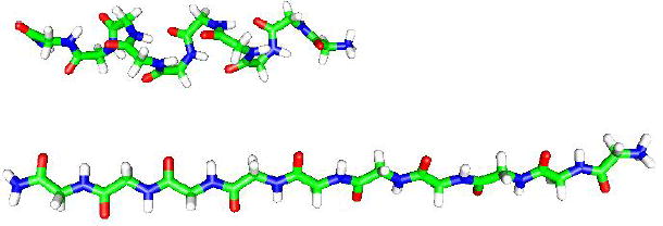
A picture (generated using gOpenMol) of the peptide subjected to external forces (in the horizontal direction in the picture) of K=2 and 100 kcal/(mol·Å). For K=2 the molecule is still approximately helical with end-to-end distance of R=21.7 Å. For K=100 kcal/(mol·Å) the helix becomes an extended structure that is stretched significantly to R=36.8 Å with decreased conformational freedom. This is a pictorial illustration for the results of Δα_k (Table 1), which are shown to decrease as the external force increases. Similar figures for the forces K=8, 20 and 40 are not provided because the corresponding extensions are close to that of K=100 (see Table 4).

For small values of the external force the conformations remain helical during the entire simulation, but for K ≈ 4 kcal/(mol·Å) the molecule that stays initially in the helical region is transformed after a short simulation time into an extended state, the stronger is K the shorter is this time, where for large enough K the (metastable) helical state is hardly observed in the trajectory. The HSMC method is applied to samples (obtained from different values of the external force) consisting of the (most stable) extended conformations.

The TPs and their product, ρ^HS (eqs 7 and 15) were calculated by reconstructing each conformation step-by-step with MC simulations of the future part, where the geometrical restriction defined by the Δαk is applied as well. To check the convergence of the results they were calculated for four future sample sizes, n_f= 20,000, 40,000, 80,000, and 160,000, generated by retaining a conformation every 10 MC steps, and for four bin sizes, δ=Δα_k/60, Δα_k/30, Δα_k/15, and 20° centered at α_k.(i.e., α_k ±δ/2). Notice that as for the LS method, the bin size is proportional to Δα_k. If the counts of the smallest bin are smaller than 50 the bin size is increased to the next size, and if necessary to the next one (δ=Δα_k/15), etc.. In the case of zero counts, n_visit is taken to be 1; however, zero counts is a very rare event. Samples of 600 structures for K=8, 20, 40 and 100 kcal/(mol·Å) were analyzed using HSMC and the corresponding entropy and free energy results are summarized in Tables 2 and 3.

Table 2.

Entopy, TS^A (T=300 K) in kcal/mol (eq 11) for various bin sizes (eq 5) and future sample sizes, n_f, obtained with the HSMC method for different values of the external force, K^*

Bin size	nf	K=8	K =20	K =40	K =100
Δαk/30	20,000	99.9 (3)	96.5 (2)	92.6 (4)	89.2 (3)
"	40,000	99.4 (3)	96.3 (1)	92.6 (3)	89.1 (3)
"	80,000	99.3 (3)	96.2 (2)	92.7 (3)	89.2 (3)
"	160,000	99.3 (2)	96.2 (2)	92.7 (3)	89.2 (3)
Δαk/60	20,000	99.4 (3)	96.0 (2)	92.1 (4)	88.7 (3)
"	40,000	99.1 (2)	96.0 (2)	92.3 (3)	88.8 (3)
"	80,000	99.1 (2)	95.9 (1)	92.4 (3)	88.9 (3)
"	160,000	99.1 (2)	95.9 (2)	92.4 (3)	88.9 (3)
TSQH		110.2 (4)	106.5 (3)	104.2 (4)	98.0 (5)
TSLS		114.7 (5)	110.1 (3)	105.9 (4)	101.4 (5)

^*Δα_k is defined in eq 8. The HSMC results are based on a sample of 600 conformations. K is given in kcal/(mol·Å). The statistical errors are given in parentheses, e.g., 99.1 (3) = 99.1 ±0.3. S_QH is the quasi-harmonic entropy (eq 21) and S_LS (eqs 11 and 13) is the local states (LS) entropy obtained for b=1 and l=10. The entropy is defined up to an additive constant.

Table 3.

HSMC results for various free energy functionals for four different values of the external force K^*

	K=8			K=20			K=40			K = 100
HSMC/ nf	-FA	-FB	σA	-FA	-FB	σA	-FA	-FB	σA	-FA	-FB	σA
20,000	422.7(5)	415.1	3.4	845.3(2)	836.2	2.9	1558.7(6)	1547.4	3.7	3744.3(6)	3734.4	3.9
40,000	422.4(4)	415.3	2.9	845.3(2)	836.6	2.5	1558.9(6)	1547.9	3.2	3744.4(6)	3737.1	3.2
80,000	422.3(4)	416.1	2.7	845.2(2)	836.3	2.2	1559.0(6)	1548.6	3.2	3744.5(6)	3737.9	2.7
160,000	422.3(4)	416.9	2.7	845.2(2)	837.3	2.2	1559.0(6)	1548.4	3.2	3744.5(6)	3738.3	2.5
-FD -FM	418.6	419.6		840.1	841.3		1551.5	1553.7		3740.5	3741.4
-FQH	426.9 (2)			852.4 (2)			1569.0 (2)			3750.9 (4)
-FLS	431.3 (4)			856.0 (2)			1570.6 (3)			3754.3 (4)
Eint	−43.5 (2)			−39.5 (4)			−27 (1)			23.1 (8)
- Etot	323.3 (3)			749.3 (3)			1466.6 (5)			3655.6 (3)

^*F^A (eq 12) and F^B (eqs 16 and 17) are lower and upper bounds of the free energy, respectively, and σ_A (eq 14) is the fluctuation of FA. These HSMC results were obtained from samples of 600 conformations. These results are presented only for the smallest bin size, δ=Δα_k/60, but for all future sample sizes n_f. The results for F^M (eq 18) - the average of F^A and F^B, and for F^D (eq 20) - the exact free energy functional, are calculated for δ=Δα_k/60 and n_f =160,000 only. F_QH (eq 21) and F_LS (eq 12) are free energies obtained by the quasi-harmonic approximation and the local states method, respectively, and are based on larger samples (see text). The average potential energy, E_int and the total energy, E_int = E_int +E_ext of the HSMC samples (in kcal/mol) appear in the bottom rows. All free energies (at T=300 K) are in kcal/mol and are defined up to an additive constant. K is given in kcal/(mol·Å). The statistical error is defined in the caption of Table 2. We estimate the errors in F^B and F^D to be larger than the corresponding errors in F^A at least by a factor of three and two, respectively.

B. Results for the entropy

It should first be pointed out that as for the dihedral angles, eq 15 was used with δα_k also for the bond angles, i.e., without considering the Jacobian component [Π_ksin(θ_k)], because we have found that to a good approximation, the contribution of the Jacobian to the entropy cancels out in entropy and free energy differences, which are our main interest.

Table 2 contains results (at T=300 K) for the entropy, TS^A (eq 11) for four different external forces. For each force 600 configurations (out of the entire sample size of 2500) were analyzed, and the results were calculated for four different future sample sizes n_f and four bin sizes. However, the extent of convergence of these results is demonstrated by the best ones, i.e., those for the two smallest bin sizes, Δα_k/60 and Δα_k/30 and therefore only they are presented in the table. Results were calculated for partial samples of size, 100, 200, 300, 400, 500 and 600, where typically the entropy (S^A) and energy for sample sizes 300–600 have been found to converge, i.e., to fluctuate slightly around an average value; the statistical errors were obtained from these fluctuations.

The accuracy of HSMC can always be improved by decreasing the bin size and increasing the future sample size, meaning that the corresponding S^A is expected to decrease, provided that the probability density ρ^HS is defined on the same conformational space that was generated by MC simulation. Indeed, for K=8 and 20 the central values decrease or remain constant for each bin as n_f increases; a similar picture is shown for K=40 and 100 even though in some cases this trend is reversed due probably to insufficient equilibration for the high external forces for the smaller n_f values (20000, and 40000), which leads to elevated S^A results. However, almost always these differences are insignificant within the statistical errors, meaning that for the present accuracy a future sample of 80,000 and even 40,000 is sufficient.

As expected, the values for the smallest bin, Δα_k/60 are slightly lower than the corresponding values for Δα_k/30 (even though in most cases the differences are covered by the error bars) meaning that convergence has not been attained completely with respect to the bin size; however, the differences T[S^A (Δα_k/30) − S^A (Δα_k/60)] for n_f =160,000 are almost equal, 0.2–0.3 kcal/mol for all forces, i.e., the extent of convergence is about the same and therefore correct entropy differences are expected to be obtained from differences in S^A. In fact, the molecule is already relatively stiff for K=8 and the change, T[S^A (K=100) − S^A (K=8)] ≈ 10 kcal/mol is therefore relatively small as well.

The HSMC entropy results (TS^A) are compared in the table with those obtained using the LS method and the quasi-harmonic (QH) approximation. For this we generated larger samples of sizes 15,000 and 30,000 for the QH and LS, respectively imposing the geometric restriction as explained earlier. As expected, both methods lead to results that are larger than the HSMC values, by up to 15 kcal/mol, i.e., ~15% (LS, using b=1 and l=10) and 12 kcal/mol (QH).

C. Results for the free energy

Results for the free energy functional, F^A (eq 12) and its fluctuation, σ_A (eq 14), F^B [Eqs. (16) and (17)], F^D (eq 20) and the energies are presented in Table 3. These results are given only for the smallest bin, because F^A values for the bin, Δα_k/30 can be obtained from the entropies of Table 2 and the energies provided in the bottom of Table 3.

The results for F^A follow the opposite trend observed in Table 2 for the entropy, i.e. for K=8 and K=20 F^A increases or remains unchanged, as the sample size n_f increases, in accordance with F^A being a lower bound; for K=40 and K =100 this trend is changed some times according to the behavior of S^A discussed in the previous section. As for S^A, differences in F^A are expected to represent faithfully the exact ones. The values of σ_A, as expected, decrease or remain unchanged as the future sample size increases, but within relatively large statistical errors.

The results for F^B (eqs 16 and 17) (that constitutes an upper bound for the free energy) indeed in most cases show the expected decrease as n_f is increased and they are larger than the F^A values. However, the corresponding values for the larger bin, Δα_k/30 (not shown) are smaller than those presented in the table (for Δα_k/60), which suggests that the F^B results are not yet statistically converged, i.e., much larger samples are needed; also, it is difficult to calculate their statistical errors, which we estimate to be at least three times larger than the corresponding errors presented for F^A. The same discussion applies to F^D, which is expected, however, to be statistically more reliable than F^B; we estimate its errors to be at least twice as large as those presented for F^A(n_f = 160,000). Still, we present the results for F^M, the average of F^A and F^B, which are close to the F^D values (maximum difference ~1.5 kcal/mol), and constitute estimates for the correct free energy; the differences, F^M − F^A are ~2.7, 3.9, 5.3, and 3.1 kcal/mol for K=8, 20, 40, and 100, respectively and we expect the correct values to be closer to F^A than to F^M. Although these differences might seem large, the relative differences are small (smaller than 0.6% and for K=100 ~0.08 %). Since the relatively large external force (see table 3) sets the scale for the free energy of the system, the contribution of the entropy to the absolute free energy as well as to free energy differences for various external forces is quite small. As for the entropy, the QH and LS results constitute a significant underestimation of the free energy.

The results shown thus far suggest that the model of peptide used is quite stiff. This is also demonstrated in Table 4 by the relatively small increase in the extension (ΔR=1.8 Å) in going from K=8 to K=100, and a relatively small (expected) decrease in the corresponding entropy by TΔS= ~10 kcal/mol. On the other hand, the change in the potential energy is relatively large ΔE_int = ~66 kcal/mol, due to strong bond angle potentials, and the change in the energy due to the external force is 1.8·92~166 kcal/mol.

Table 4.

HSMC results for extensions, R, entropies, TS^A, and potential energies, Eint, for different external forces, K, at T=300 K^*

K [kcal/(mol·Å)]	R (Å)	TS [kcal/mol]	Eint [kcal/mol]
8	34.98 (3)	99.1 (2)	−43.5 (2)
20	35.49 (2)	95.9 (2)	−39.5 (4)
40	35.99 (2)	92.4 (3)	−27 (1)
100	36.78 (2)	88.9 (3)	+23.1 (8)

^*The statistical error is defined in Table 2.

D. Results from thermodynamic integration and free energy derivatives

The relatively small changes in the entropy as the forces increase are also shown in Table 5, where they are compared with results obtained by thermodynamic integration using eq 23. The latter results were calculated as follows: the segment [K_i, K_i+1] was divided into 20 equal values, and for each value an MC sample of 600 structures was generated (imposing the Δα_k restrictions) where the corresponding extension R was calculated. The difference in entropy was calculated from the area below the K(R) function by a numerical integration technique. It should be pointed out, that while the HSMC and the integration values for the entropy differences are equal within the statistical errors, the integration errors are relatively large because we have found the integration results to be sensitive to the sample size (we studied samples between 600 –5000 conformations).

Table 5.

Differences in the entropy, T S^A, (kcal/mol) at T=300 K for different forces, K obtained by HSMC and by integration using eq 23^*

	HSMC	Integration
T[SA(K=8) - SA(K=20)]	3.2 (1)	3.1 (2)
T[SA(K=20) - SA(K=40)]	3.5 (2)	3.0 (5)
T[SA(K=40) - SA(K=100)]	3.5 (2)	3.8 (5)

^*The statistical error is defined in Table 2.

Another test for the reliability of the HSMC results is based on eq 22. Thus, we generated two samples of 200 structures for K=7 and 9 and calculated the corresponding values of F^A, from which R_d = − [F^A(9)− F^A(7)]/2 was calculated. Indeed R_d is very close to both R(K=8) (Table 4) and the average of R(9) and R(7) obtained from the two samples. Reconstructing a single conformation of (Gly)₁₀ based on n_f = 160,000 requires ~240 minutes CPU time on a 2.6 GHz Athlon processor. Obviously, application of HSMC to a sample of size n can be carried out in parallel on n processors.

VI. Summary

In this paper we have applied the HSMC method to the flexible model of decaglycine in the helical conformation (at T=300 K) subjected to a stretching external force. However, for forces larger than a small critical value a transition from the helix to the extended state occurs already in the early stage of the MC simulation and the entropy and free energy were therefore obtained for the extended state. The present results are more accurate than those obtained by the LS and QH methods, and it is of interest to compare them also to results obtained for the flexible model of (Gly)₁₀ in Ref. 25 at T=100 K without applying external forces. Thus, the accuracy of S^A, the upper bound of the entropy, is better than that obtained there for the hairpin and is slightly worse than that obtained for the helix and extended states. However, the results for F^B and F^D are less accurate than those found for the un-stretched peptides.²⁵ It should be noted that because of the decrease in the conformational space due to the forces, the smallest bin size was decreased from Δα_k/15 in Ref. 25 to Δα_k/60 in the present study. We have also found that the MC acceptance rate should be ~0.4.

The molecule is found to be relatively stiff due to the strong bond angle potentials, which is reflected by the relatively small extension obtained by increasing the force by a factor of 10; the corresponding decrease in the entropy, as expected, was small as well. In other words, the contribution of the entropy to differences in the free energy is significantly smaller than the contribution of the external and internal energies. Still, differences in entropy for the different forces are calculated with acceptable errors that are not larger than 0.2 kcal/mol.

The present study constitutes the initial application of HSMC to a peptide under stretching forces, therefore we have chosen a molecule (decaglycine) that is much smaller and simpler than the molecules typically studied by AFM; however, simple small peptides under a stretching force have been also simulated by others,^41,42,54 and experiments on relatively small proteins have been carried out.⁵⁵ Because the time frame of AFM experiments is in the millisecond to second range,³⁷ the force exerted is changed relatively slowly, leading approximately to a reversible process. SMD simulations, on the other hand, are limited to the nanosecond time frame and therefore require much stronger (and rapidly changed) forces that lead to an irreversible mechanical work significantly larger than the corresponding reversible work. Calculating the reversible work (from irreversible SMD trajectories) has been the subject of several recent papers,^44,45,54 but it can alternatively be obtained by HSMC using eq 23, where state 1 corresponds to zero force and state 2 to any force of interest along the SMD trajectory. The irreversible work can be obtained by integrating K(R) (eq 23) and the difference between the reversible and irreversible works thus calculated; these works can be compared to that generated in the experiment.

The present results demonstrate further the versatility of the HSMC method, which has been applied thus far to liquid argon and TIP3P water,^22.23 self avoiding walks on a lattice,²⁶ and models of decaglycine.^24,25 To further enhance the performance of HSMC we are extending it now to molecular dynamic (rather than MC) simulations, where our long-term goal is to develop software that enables one to apply the method to a general peptide consisting of any sequence of amino acid residues in implicit as well as explicit solvent. HSMC will then be used to study the effect of surface loops flexibility on protein function, and will become an ingredient of procedures for free energy based docking of flexible ligands to an active site of an enzyme; thus, HSMC will become a useful tool also in protein engineering. When applied with MD, the scope of HSMC will be extended to more complex problems involving macromolecular stretching, where the calculation of free energy and potential of mean force profiles is of interest, as discussed in some detail above.

Table 6.

Calculation of the extension, R for external force, K=8 from free energy results (F ) obtained by HSMC for K=7 and K=9 using the derivative, eq 22^*

F(K=7) (kcal/mol)	F(K=9) (kcal/mol)	-ΔF/ΔK (Å)	[R(K=9)+R(K=7)]/2 (Å)	R(K=8) (Å)
−387.5 (4)	−457.7 (4)	35.1 (4)	34.96 (3)	34.98 (3)

^*K is given in kcal/(mol·Å). The free energy values were obtained from samples of 200 configurations. The statistical error is defined in the caption of Table 2.

References

- 1.Metropolis N, Rosenbluth AW, Rosenbluth MN, Teller AH, Teller E. J Chem Phys. 1953;21:1087. [Google Scholar]
- 2.Alder BJ, Wainwright TE. JChem Phys. 1959;31:459. [Google Scholar]
- 3.McCammon JA, Gelin BR, Karplus M. Nature. 1977;267:585. doi: 10.1038/267585a0. [DOI] [PubMed] [Google Scholar]
- 4.Beveridge DL, DiCapua FM. Annu Rev Biophys Biophys Chem. 1989;18:431. doi: 10.1146/annurev.bb.18.060189.002243. [DOI] [PubMed] [Google Scholar]
- 5.Kollman PA. Chem Rev. 1993;93:2395. [Google Scholar]
- 6.Jorgensen WL. Acc Chem Res. 1989;22:184. [Google Scholar]
- 7.Meirovitch, H. Reviews in Computational Chemistry, edited by Kenny B. Lipkowitz and Donald B. Boyd (Wiley, New York, 1998), vol.12 p.1
- 8.Szarecka A, White RP, Meirovitch H. J Chem Phys. 2003;119:12084. [Google Scholar]
- 9.White RP, Meirovitch H. J Chem Phys. 2003;119:12096. [Google Scholar]
- 10.Duan Y, Kollman PA. Science. 1998;282:740. doi: 10.1126/science.282.5389.740. [DOI] [PubMed] [Google Scholar]
- 11.Meirovitch H. Chem Phys Lett. 1977;45:389. [Google Scholar]
- 12.Meirovitch H. Phys Rev B. 1984;30:2866. [Google Scholar]
- 13.Meirovitch H, Vásquez M, Scheraga HA. Biopolymers. 1987;26:651. doi: 10.1002/bip.360260508. [DOI] [PubMed] [Google Scholar]
- 14.Meirovitch H, Koerber SC, Rivier J, Hagler AT. Biopolymers. 1994;34:815. doi: 10.1002/bip.360340703. [DOI] [PubMed] [Google Scholar]
- 15.Chorin AJ. Phys Fluids. 1996;8:2656. [Google Scholar]
- 16.Meirovitch H. J Phys A. 1983;16:839. [Google Scholar]
- 17.Meirovitch H. Phys Rev A. 1985;32:3709. doi: 10.1103/physreva.32.3709. [DOI] [PubMed] [Google Scholar]
- 18.Meirovitch H, Scheraga HA. J Chem Phys. 1986;84:6369. [Google Scholar]
- 19.Meirovitch H. J Chem Phys. 1992;97:5816. [Google Scholar]
- 20.Meirovitch H. J Chem Phys. 1999;111:7215. [Google Scholar]
- 21.Meirovitch H. J Chem Phys. 2001;114:3859. [Google Scholar]
- 22.White RP, Meirovitch H. Proc Natl Acad Sci USA. 2004;101:9235. doi: 10.1073/pnas.0308197101. [DOI] [PMC free article] [PubMed] [Google Scholar]
- 23.White RP, Meirovitch H. J Chem Phys. 2004;121:10889. doi: 10.1063/1.1814355. [DOI] [PubMed] [Google Scholar]
- 24.Cheluvaraja S, Meirovitch H. Proc Natl Acad Sci USA. 2004;101:9241. doi: 10.1073/pnas.0308201101. [DOI] [PMC free article] [PubMed] [Google Scholar]
- 25.Cheluvaraja S, Meirovitch H. J Chem Phys. 2005;122:054903–1. doi: 10.1063/1.1835911. [DOI] [PubMed] [Google Scholar]
- 26.White RP, Funt J, Meirovitch H. Chem Phys Lett. 2005;410:430. doi: 10.1016/j.cplett.2005.06.002. [DOI] [PMC free article] [PubMed] [Google Scholar]
- 27.Cornell WD, Cieplak P, Bayly CI, Gould IR, Merz KM, Jr, Ferguson DM, Spellmeyer DC, Fox T, Caldwell JW, Kollman PA. J AmChem Soc. 1995;117:5179. [Google Scholar]
- 28.Karplus M, Kushick JN. Macromolecules. 1981;14:325. [Google Scholar]
- 29.Rojas OL, Levy RM, Szabo A. J Chem Phys. 1986;85:1037. [Google Scholar]
- 30.Mark, J.E.; Erman, B. “Rubberlike Elasticity, a Molecular Primer”. John Wiley, 1988.
- 31.Florin EL, Moy VT, Gaub HE. Science. 1994;264:415. doi: 10.1126/science.8153628. [DOI] [PubMed] [Google Scholar]
- 32.Rief M, Gautel M, Oesterhelt F, Fernandez JM, Gaub HE. Science. 1997;276:1109. doi: 10.1126/science.276.5315.1109. [DOI] [PubMed] [Google Scholar]
- 33.Merkel R, Nassoy P, Leung A, Ritchie K, Evans E. Nature. 1999;397:50. doi: 10.1038/16219. [DOI] [PubMed] [Google Scholar]
- 34.Li H, Oberhauser AF, Fowler SB, Clarke J, Fernandez JM. Proc Natl Acad Sci USA. 2000;97:6527. doi: 10.1073/pnas.120048697. [DOI] [PMC free article] [PubMed] [Google Scholar]
- 35.Kellermayer MSZ, Smith SB, Granzier HL, Bustamante C. Science. 1997;276:1112. doi: 10.1126/science.276.5315.1112. [DOI] [PubMed] [Google Scholar]
- 36.Izrailev S, Stepaniants S, Balsera M, Oono Y, Schulten K. Biophys J. 1997;72:1568. doi: 10.1016/S0006-3495(97)78804-0. [DOI] [PMC free article] [PubMed] [Google Scholar]
- 37.Isralewitz B, Gao M, Schulten K. Curr Opin Struct Biol. 2001;11:224. doi: 10.1016/s0959-440x(00)00194-9. [DOI] [PubMed] [Google Scholar]
- 38.Gao M, Wilmanns M, Schulten S. Biophys J. 2002;83:3435. doi: 10.1016/S0006-3495(02)75343-5. [DOI] [PMC free article] [PubMed] [Google Scholar]
- 39.Paci E, Karplus M. J Mol Biol. 1999;288:441. doi: 10.1006/jmbi.1999.2670. [DOI] [PubMed] [Google Scholar]
- 40.Evans E, Ritchie K. Biophys J. 1997;72:1541. doi: 10.1016/S0006-3495(97)78802-7. [DOI] [PMC free article] [PubMed] [Google Scholar]
- 41.Cieplak M, Hoang TX, Robbins MO. Proteins: Struct, Funct,Genet. 2002;49:104. doi: 10.1002/prot.10188. [DOI] [PubMed] [Google Scholar]
- 42.Bryant Z, Pande VS, Rokhsar DS. Biophys J. 2000;78:584. doi: 10.1016/S0006-3495(00)76618-5. [DOI] [PMC free article] [PubMed] [Google Scholar]
- 43.Essevaz-Roulet B, Bockelmann U, Heslot F. Proc Natl Acad Sci USA. 1997;94:11935. doi: 10.1073/pnas.94.22.11935. [DOI] [PMC free article] [PubMed] [Google Scholar]
- 44.Gullingsrud JR, Braun R, Schulten K. J Comp Phys. 1999;151:190. [Google Scholar]
- 45.Hummer G, Szabo A. Proc Natl Acad Sci USA. 2001;98:3658. doi: 10.1073/pnas.071034098. [DOI] [PMC free article] [PubMed] [Google Scholar]
- 46.Ponder, J.W. 2001, TINKER - software tools for molecular design, version 3.9. [DOI] [PMC free article] [PubMed]
- 47.Gô N, Scheraga HA. J Chem Phys. 1969;51:4751. [Google Scholar]
- 48.Gô N, Scheraga HA. Macromolecules. 1976;9:535. [Google Scholar]
- 49.Baysal C, Meirovitch H. Biopolymers. 1999;50:329. doi: 10.1002/(SICI)1097-0282(199909)50:3<329::AID-BIP8>3.0.CO;2-4. [DOI] [PubMed] [Google Scholar]
- 50.Meirovitch H, Alexandrowicz Z. J Stat Phys. 1976;15:123. [Google Scholar]
- 51.Meirovitch H. J Chem Phys. 1988;89:2514. [Google Scholar]
- 52.Meirovitch H, Vásquez M, Scheraga HA. Biopolymers. 1988;27:1189. doi: 10.1002/bip.360270802. [DOI] [PubMed] [Google Scholar]
- 53.Hill, T.L. Statistical Mechanics Principles and Selected Applications. Dover, New York. 1956.
- 54.Park S, Khalili-Araghi F, Tajkhorshid E, Schulten K. J Chem Phys. 2003;119:3559. [Google Scholar]
- 55.Yang G, Cecconi C, Baase WA, Vetter IR, Breyer WA, Haack JA, Matthews BW, Dahlquist FW, Bustamante C. Proc Natl Acad Sci USA. 2000;97:139. doi: 10.1073/pnas.97.1.139. [DOI] [PMC free article] [PubMed] [Google Scholar]