Precise Boundary Element Computation of Protein Transport Properties: Diffusion Tensors, Specific Volume, and Hydration

Abstract

A precise boundary element method for the computation of hydrodynamic properties has been applied to the study of a large suite of 41 soluble proteins ranging from 6.5 to 377 kDa in molecular mass. A hydrodynamic model consisting of a rigid protein excluded volume, obtained from crystallographic coordinates, surrounded by a uniform hydration thickness has been found to yield properties in excellent agreement with experiment. The hydration thickness was determined to be δ = 1.1 ± 0.1 Å. Using this value, standard deviations from experimental measurements are: 2% for the specific volume; 2% for the translational diffusion coefficient, and 6% for the rotational diffusion coefficient. These deviations are comparable to experimental errors in these properties. The precision of the boundary element method allows the unified description of all of these properties with a single hydration parameter, thus far not achieved with other methods. An approximate method for computing transport properties with a statistical precision of 1% or better (compared to 0.1–0.2% for the full computation) is also presented. We have also estimated the total amount of hydration water with a typical −9% deviation from experiment in the case of monomeric proteins. Both the water of hydration and the more precise translational diffusion data hint that some multimeric proteins may not have the same solution structure as that in the crystal because the deviations are systematic and larger than in the monomeric case. On the other hand, the data for monomeric proteins conclusively show that there is no difference in the protein structure going from the crystal into solution.

INTRODUCTION

The crystal structure of proteins can be readily determined by x-ray diffraction methods (1,2), as long as they can be crystallized. Protein function occurs while immersed in liquid aqueous environment, and a significant amount of water of hydration is associated with the protein in solution. Since proteins crystallize with a significant amount of their water of hydration, it is reasonable to assume that the solution structure and crystal structures are about the same. To test this hypothesis experimentally, one needs to compare precisely computed transport properties derived from the crystal structure with those measured in solution. Many methods exist to probe the structure and dynamics of molecules in solution, including dynamic laser light scattering (3), transient electric birefringence (4), fluorescence polarization anisotropy (5), fluorescence photobleaching recovery (6), electron spin resonance (7), and nuclear magnetic resonance (8). These modern techniques emphasize the dynamics of the molecules in solution at timescales characteristic of each technique. Classical techniques such as centrifugation and electrophoresis are also important for biomolecules (9). The characteristic time constants for the slower molecular dynamics process are often quite well described as diffusive in origin and thus directly relate to the hydrodynamic friction tensors of the molecule in question. In a previous article (10), we have reported on the development of a very precise boundary element method (BE), and a program suite (BEST) for the computation of transport tensors of macromolecules under the stick boundary condition. In this article, we report on the use of BEST for the determination of the thickness of the hydration layer, the specific volume, and the translational and rotational diffusion coefficients of a large suite of soluble proteins.

Several authors (11–15) have published work addressing this same topic with a variety of computational methods in the past. The classical work based on effective ellipsoids to represent protein shape clearly showed that much more detailed surface representation was needed to be able to predict reasonable water of hydration numbers, for example. An advance was made with the introduction of coarse hydrodynamically interacting bead methods, but these cannot simultaneously predict correct translation and rotational diffusion properties (16) because the model is still too approximate, with errors typically around 15%. A model that treats the protein in atomistic detail is needed.

Garcia de la Torre et al. (17) have further developed the “shell” model originally suggested by Teller (18). In this method, very small equal-sized beadlets are placed on the surface of the body to be modeled, avoiding any overlapping beads. Then, by assigning multiple beads to the solvent accessible surface of atoms, a bead model could produce an acceptable atomistic transport coefficient in the limit of zero bead size. Since the hydrodynamic interaction tensors are only approximate, however, this method requires a different parametrization depending on which transport property is being addressed. If we are to focus on the surface of the body, then we are better off using an exact representation of the transport properties without reference to beads at all. The work of Garcia de la Torre arrives at an estimate for the water of hydration of proteins of ∼1.2 Å thick layer.

Recently, Allison (19,20) and Zhou (21) have reintroduced the hydrodynamic BE method originally formulated by Youngren and Acrivos (22) to address this problem. Allison (20) studied lysozyme to show that the BE method was applicable, but his focus was the electrophoretic mobility and he did not try to determine the hydration thickness. Zhou (21) was the first to specifically demonstrate, in a small study of four proteins, that taking into account the specific protein shape by BE methods could lead to a hydrodynamic picture consistent with other methods for determining water of hydration. Zhou's value for the hydration thickness, however, is somewhat small (0.9 Å) because his use of the molecular van der Waals surface allowed more hydration water to be present. The van der Waals surface is the exterior of a set of overlapping spheres that have small crevasses between some neighboring spheres. If this surface is used, then the hydrodynamic computation will place water in these crevasses. However, a water molecule has a finite size and in reality will not fit into such small spaces. Thus, we have chosen a hydrodynamic surface as defined by the Connolly procedure to avoid this problem. The procedure is detailed below. In addition, Kim (23) has developed an alternative BE method where he formulates the problem by means of the double layer integrals to avoid the ill conditioning of the direct Youngren-Acrivos method. In our previous work (10), however, we have developed an excellent regularization method that deals very effectively with the ill-conditioned problem. This method is called the “area correction” and this is incorporated into our program BEST. With this methodology, we can now do numerically exact microhydrodynamics.

THEORY: THE BOUNDARY ELEMENT METHOD FOR STICK BOUNDARY CONDITIONS

For macromolecules, consideration of the solvent as a continuum is an excellent approximation, and the governing equations for the computation of the hydrodynamic transport properties are the Navier-Stokes equations of fluid flow. In the limit of small Reynolds number, as appropriate for the diffusion process, the equations are known as the Stokes or creeping flow equations (24). Whereas bead methods aim to solve a mobility problem that cannot be formulated exactly, an alternative method is to solve a resistance problem, which can be formulated exactly as an integral equation. As is shown below, once one has precise friction tensors, it is straightforward to compute the diffusion tensors. In the mid '70s, Youngren and Acrivos (22) presented an effective method for the numerical solution to the exact surface integral representation of the velocity field for the creeping flow equations. The method implemented in BEST corresponds to the equations described below.

In the following, we review the equations of the Youngren-Acrivos (22) method. For the case of macromolecules, “stick” boundary conditions are appropriate. In this case, the velocity field of the flow, at position in the fluid, can be written as an integral over the particle surface (SP),

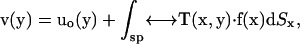(1)

where is the flow velocity of the fluid if the particle was not there (which can be taken to be zero for diffusive motion), and is the Oseen hydrodynamic interaction tensor. The surface stress force, , is the unknown quantity that we must obtain. Once this quantity is known, the transport properties of the macromolecule can be directly computed, as shown below. The Oseen tensor is given by (25,26)

(2)

It is important to note that in bead hydrodynamics, the Oseen tensor is only the first term in an infinite series expansion of the interaction between two beads centered at and , respectively. However, when the hydrodynamics is expressed as a continuous integral over the surface of the body, the tensor is an exact representation of the hydrodynamic interaction of the infinitesimal surface elements. Thus the starting expressions for the calculation, unlike the bead modeling case, are exact (22,27); moreover, the equation is applicable to bodies of arbitrary shape.

Since Eq. 1 is an integral equation, the solution requires an approximate numerical method. The method, however, can be iterated to obtain arbitrary precision. The first step is to discretize the surface by replacing it with a collection of N patches that smoothly tile the molecular surface. We can then write,

(3)

We place the coordinate _j at the center of the small patch and take the surface stress force to be a constant over the entire patch area. This is the basic approximation: it is clear that it will become a better and better approximation as the patch is made small. Thus, an extrapolation to zero size patch leads to a very precise value for the transport properties. With this approximation, Eq. 1 becomes a set of 3N equations for 3N unknowns ,

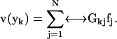(4)

The centerpiece of this set of equations is a set of N completely known 3 × 3 matrices of coefficients that contain all geometric information, the integrals of the Oseen tensor over a surface patch,

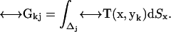(5)

In addition to the introduction of a robust regularization method, the other significant advance made in our work is the essentially exact integration of the Oseen tensor in the above expression. The set of 3N equations can be written all at once,

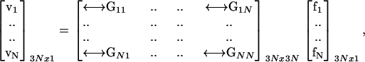(6)

from which the unknown surface stress forces can be readily obtained by matrix inversion of the 3N × 3N super matrix ,

(7)

The total force and torque on the body can be computed from the surface stress forces and these are directly related to the friction tensors () of the body,

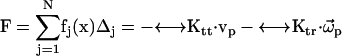(8)

(9)

The particle can be assumed to have specific translation velocity and angular velocity ω_p (for example ω_p = 0 and = (v_x,0,0)) to solve the above equations. Thus, six calculations suffice to determine all components of the friction tensors. The friction tensors form part of a larger 6 × 6 tensor that contains information about the pure translational friction (tt), the pure rotational friction (rr) and the coupling that may exist between these (rt and tr). There are actually only three independent friction tensors because the tensor is the transpose of the tensor. This coupling is insignificant unless the body has a screw-like axis of symmetry (28). The diffusion tensors are finally obtained from the friction tensors by an easy 3 × 3 matrix inversion,

(10)

(11)

BEST computes diffusion tensors in the Center of Diffusion and the friction tensors in the Center of Resistance. Details are presented in Aragon (10).

PROTEIN HYDRATION AND SPECIFIC VOLUME

Protein hydration can be determined by a variety of methods and has been reviewed extensively in the literature (29–31). Measurements determine the weight of water per gram of protein and which is denoted h in this work. This value varies somewhat, but is typically h 0.3–0.4 g water/g protein, and it was noticed in the early work (30), which represented proteins by effective ellipsoids, that values from hydrodynamics varied greatly and could be much larger than determined by other methods. This work and that of Zhou (21) establish that the principal source of the large variation is the ellipsoid representation of the shape. Hydrodynamic methods depend on the shape of the volume that exerts friction with the solvent. Thus, the thickness of the hydration layer is the proper parameter of our model. We make the simplifying assumption that the water is distributed uniformly over the surface of the protein for all soluble proteins, and we determined, by comparison with experiment, that this assumption is quite reasonable.

The Connolly MSROLL program (32–34) can triangulate only the molecular surface; thus we had to define our hydrated surface differently than the Connolly concept of the solvent accessible surface. To define the hydrated surface, we used the simple process of enlarging the atomic radii of the constituent protein atoms, as found in the Brookhaven crystallographic database. The hydrated surface (a new molecular surface) and the unmodified molecular surface are determined by means of the MSROLL program of Connolly, with a probe radius of 1.5 Å to represent water. The molecular surface is defined by the Connolly surface obtained from the van der Waals radii of the protein atoms (see Fig. 1). Since hydrogen is typically not detected in the crystal structure, we used the modified set of radii built in to MSROLL that contain slightly enlarged heteroatoms when these have hydrogen bonded to them. The volume enclosed by the molecular surface is the protein excluded volume, V₀. To represent hydration, we add a thickness δ to all radii, and perform the Connolly roll once more. The larger surface so obtained is the hydrated surface, and the hydration volume, V_h, is the difference between the volume enclosed by the hydrated surface, V(δ) and the excluded volume of the protein: V_h = V(δ) − V₀ . Using the known slightly larger value of the hydration water density (35) of ρ_h = 1.1 g cm⁻³, we can compute hydration h = V_h ρ_h N₀/M_W, from Avogadro's number and the protein molecular weight. Fig. 2 shows a typical crystallographic structure and a corresponding triangulation of the surface by MSROLL. We note that the inflated molecular surface so generated is somewhat arbitrary and it is ultimately just a means to enable the accurate computation of hydrodynamic transport coefficients.

FIGURE 1.

(A) Connolly ball rolling over the atoms defines the molecular surface, which encloses the protein-excluded volume, V₀. (B) To represent hydration, the atomic radii are increased by an amount δ and the Connolly ball is rolled over the atoms again. The new larger volume, V(δ), is surrounded by the hydrated surface.

FIGURE 2.

Lysozyme: space-filled model (2CDS) and triangulation of molecular surface by MSROLL.

We must determine the hydration thickness, δ, by comparison with experimental transport properties. For this purpose, we selected a set of four small proteins whose translational diffusion coefficients have been well determined: lysozyme, ribonuclease, myoglobin, and chymotripsinogen A. For each protein, the parameter δ was varied to obtain a set of surfaces with varying hydration thickness. Each one of these surfaces was then triangulated with MSROLL. Furthermore, to eliminate the discretization error and to regularize the solution of the integral Eq. 1, we generate, for each surface of fixed δ, a set of subtriangulations with a varying number of triangles, N. This procedure is carried out by our program COALESCE, which in addition eliminates triangles unsuitable (due to size and/or shape) for computational boundary elements. The diffusion coefficients computed by BEST are extrapolated versus 1/N to an infinite number of triangles. An example of such an extrapolation for ribonuclease is given in Fig. 3. Furthermore, Fig. 4 demonstrates that the translational diffusion coefficient does vary with hydration thickness and that the variation is well characterized by our method. Thus, there is sufficient sensitivity to be able to determine this parameter with accuracy.

FIGURE 3.

Linear extrapolation of the trace of the translational diffusion tensor for ribonuclease versus 1/N. N varies between 2590 and 4950 triangles. A linear least-squares fit to the data (cm²/s) yields an intercept of 1.0832 10⁻⁶ (standard error = 2.6 10⁻¹⁰, Tstat = 4189), a slope of 3.50 10⁻⁵ (standard error = 8.7 10⁻⁷, Tstat = 40), and a variance of 1.38 10⁻²⁰. Tstat is the T statistic indicating the appropriateness of a linear fit. The statistical error in the intercept is 0.024%.

FIGURE 4.

Graph of the translational diffusion coefficient as a function of hydration layer thickness for myoglobin (○), lysozyme (•), and chymotrypsinogen (▪).

By comparing the computed translational diffusion coefficients with the experimental values, we determine that δ = 1.1 ± 0.1 Å, a very precise value. The data are presented in Table 1. We can immediately appreciate that when we match the average translational diffusion coefficient, we also automatically match the rotational diffusion coefficient to within experimental error. In addition, the hydration h is reasonably well reproduced. Thus, the precise BE method is capable of reproducing various quantities in agreement with experiment with a universal parameter δ, something bead methods are not capable of doing (17).

TABLE 1.

Diffusion coefficients for protein test suite (δ = 1.1 ± 0.1 Å, 20 C)

	Experimental data		Calculated data			Computed hydration (gH2O/g protein)	Measured hydration (gH2O/g protein)
Protein	Dt 107cm2/s	Dr 105 s−1	Dt 107cm2/s	Dr‖ 105 s−1	Dr trace 105 s−1
Lysozyme (6LYZ)	11.2(.2)36,37	2.0(.1)38	11.0	1.9	2.16	0.325	0.3429
Chymotrypsinogen (2CGA)	9.2(.2)39	1.28(.01)40	9.24	1.22	1.26	0.303	0.3429
Myoglobin (1MBO)	10.4(.8)41	1.67(.05)42	10.2	1.62	1.74	0.314	0.4229
Ribonuclease A (7RSA)	10.68(.1)43	2.2(.1)44	10.2	1.87	2.1	0.36

Superscripts in the experimental columns indicate literature references, and uncertainties are in parentheses.

A further test of the reasonableness of the above procedure is to check that we predict values of the specific volume of proteins in agreement with experiment. The results for a large suite of proteins are given in Table 2. The specific volume of a protein is a thermodynamic quantity and it depends on several factors. Here we use a formulation due to Richards (45), in which the specific volume is the excluded volume plus corrections for the organization of water around the protein, and the breathing motions of the protein. The expression we used is

(12)

TABLE 2.

Protein-specific volume and water of hydration

			v(cm3/g)			h(g/g)
Protein	s*	Mass (kDa)	Calculated	Experimental	% error	Calculated	Experimental	% error
BPTI (5PTI)	1	6.5	0.708	0.71830	−1.3	0.414
Cytochrome c (1HRC)	1	12.4	0.713	0.71530	−0.3	0.336	0.3529	−4.0
Ribonuclease (7RSA)	1	13.7	0.695	0.70330	−0.4	0.360
Lysozyme (2CDS)	1	14.3	0.701	0.70330	−0.3	0.325	0.3429	−4.4
a-Lactalbumin (1HFX)	1	14.4	0.698	0.70447	−0.8	0.329	0.36253	−9.1
Myoglobin (1MBO)	1	17.2	0.733	0.74530	−1.4	0.348	0.4229	−17
Trypsin (1TPO)	1	23.2	0.734	0.72730	1.0	0.286
Trypsinogen (1TGN)	1	24.0	0.702	0.7348	−3.1	0.290
Chymotrypsinogen A (2CGA)	1	25.7	0.734	0.72130	1.8	0.304	0.3429	−11
Elastase (1EST)	1	25.9	0.738	0.7330	1.1	0.294
Subtilysin (1SUP)	1	27.5	0.727	0.73130	−0.6	0.260
Carbonic anhydrase B (2CAB)	1	28.7	0.708	0.73130	−2.9	0.283
Taka-amylase A (6TAA)	1	54.0	0.722	0.70049	3.1	0.223
Transferrin (1H76)	1	76.0	0.717	0.72529	−1.1	0.289
b-Lactoglobulin (1BEB)	2	36.7	0.71	0.75129	−5.3	0.294	0.2929	0
Oxyhemoglobin (1HHO)	4	64.6	0.733	0.74950	−2.1	0.295	0.3055	−1.6
Alkaline phosphatase (1ALK)	2	94.7	0.744	0.72551	2.6	0.219
Citrate aynthase (1CTS)	2	97.9	0.715	0.73352	−2.5	0.245	0.3454	−28
Lactate dehydrogenase (6LDH)	4	146.2	0.777	0.74147	4.9	0.231	0.36253	−36
Aldolase (1ADO)	4	156.0	0.759	0.74329	2.1	0.258
Catalase (4BLC)	4	232.0	0.750	0.7329	2.7	0.205	0.29053	−29

Protein Data Bank identifier in parentheses. Superscript numbers are literature references.

^*Number of protein subunits.

The first term contains the corrections for molecular breathing motions. The numerical coefficient of 0.2 Å is estimated from the standard deviation averaged over all atoms due to internal thermal motion from measurements (46) of the Rayleigh scattering of Mossbauer radiation, and S_molec (Å)² is the Connolly molecular surface area determined with MSROLL. The second term accounts for the shrinkage in volume due to the increased water density on the surface of the protein, utilizing our computed values of h. The last term comes from the excluded volume measured by MSROLL. Numerically, the last term completely dominates the expression, and the small negative second term nearly cancels the first. The agreement with experiment is excellent, with a typical discrepancy of 2% in magnitude. It is clear that the Connolly molecular surface is a very good choice to measure the excluded volume of a protein.

On the other hand, the water of hydration h does not agree as well with experiment. There are some dramatic differences, in particular for some multimeric proteins. For the monomeric proteins, the agreement is fair with an average systematic difference of −9%. This may be due to inherent difficulties in determining the experimental number, difference in conformation between the crystal and the solution phase, or the smooth layer representation. We will discuss this issue more thoroughly after we have presented the diffusion coefficient data.

PREDICTED DIFFUSION COEFFICIENTS AND COMPARISON WITH EXPERIMENT

By analyzing a small test suite, we have determined that a uniform hydration thickness yields a good description of the transport properties of those proteins, and the specific volume. We now extend the method to a much larger set of proteins where we take the hydration thickness to be fixed at 1.1 Å, as determined above. This will be a thorough test of our assumptions because now we are truly predicting protein transport properties. The computations were done as described above, including the extrapolation to an infinite number of triangles using the regularizing area correction. The results for 41 proteins are presented in Tables 3 and 4.

TABLE 3.

Protein translational diffusion coefficients (20 C)

			Dt(10−7cm2/s)
Protein*	s†	Mass (kDa)	Calculated	Experimental	References	D‡
BPTI (5PTI)	1	6.5	13.66	14.4, 14.6	56,57	−6
Cytochrome C (1HRC)	1	12.4	11.63	11.1–12.1	58–61	0
Ribonuclease A (7RSA)	1	13.7	10.84	10.68	43	2
Lysozyme (2CDS)	1	14.3	10.99	10.6, 11.2	36,37	1
a-Lactalbumin (1HFX)	1	14.4	10.84	10.57, 10.6	62,63	2
Profilin (1PNE)	1	14.8	10.74	10.6	64	1
Myoglobin (1MBO)	1	17.2	10.24	10.4, 10.5	65, 41	−2
Leghemoglobin (1LH1)	1	17.3	10.26	10.0	66	3
b-Lactoglobulin (3BLG)	1	18.4	10.07	9.7	67	4
Soybean trypsin inhibitor (1AVU)	1	21.5	9.88	9.8	68	1
Cellulase (2ENG)	1	22.0	9.63	9.8	69	−2
Somatotropin (1HGU)	1	22.1	8.84	8.88	70	0
b-Trypsin (1TPO)	1	23.3	9.50	9.3	71	2
Trypsinogen (1TGN)	1	24.0	9.49	9.68	48	−2
Chymotrypsinogen A (2CGA)	1	25.7	9.04	9.2	39	−2
Elastase (1QNJ)	1	25.9	9.22	9.5	72	−3
Savinase (1SVN)	1	26.7	9.35
Subtilysin (1SUP)	1	27.3	9.10	9.04	73	1
Carbonic anhydrase B (2CAB)	1	28.7	8.84	8.89	74	−1
Pepsin (4PEP)	1	34.5	8.10	8.01, 8.71	75,76	−3
G-actin (1NWK)	1	42.0	7.55	7.15, 7.88	77,78	0
Taka-amylase A (6TAA)	1	54.0	7.22	7.37	79	−2
Human serum albumin (1AO6)	1	69.0	6.07	5.9–6.32	80–82	−1
Superoxide dismutase (2SOD)	2	32.5	8.10	8.27	83	−2
b-Lactoglobulin (1BEB)	2	36.7	7.74	7.27, 7.34, 7.55	62, 84, 43	5
Concanavalin A (1GKB)	2	51.0	6.72	6.2	85	8
Deoxyhemoglobin (2HHB)	4	64.5	6.72	6.68	86	1
Oxyhemoglobin A (1HHO)	4	64.5	7.02	6.78	86	4
KDPG aldolase (1EUN)	3	69.2	6.22	5.6	66	11
Alkaline phosphatase (1ALK)	2	94.7	5.92	5.7	67	4
Citrate synthase (1CTS)	2	97.9	5.82	5.8	69	0
Concanavalin A (2CTV)	4	102.0	5.75	5.2, 5.6, 5.8	85, 90, 60	4
Glucose oxidase (1GPE)	2	133.7	5.45	5.02, 5.13	91, 92	7
Canavalin (2CAV)	3	141.0	5.32	5.10	90	4
Lactate dehydrogenase (6LDH)	4	145.2	5.08	4.99	30	2
Aldolase (1ADO)	4	156.0	4.66	4.29–4.8	93–96	3
Glycogen phosphorylase B (1GPB)	2	188.8	4.44	4.14	97	7
Nitrogenase MoFe (2MIN)	4	220.0	4.41	4.0	98	10
Catalase (4BLC)	4	230.3	4.49	4.1	99,100	10
Xanthine oxidase (1FIQ)	6	270.0	3.94	3.9	101	0
Glycogen phosphorylase A (1GPA)	4	377.6	3.59	3.3	97	9

^*Source for the atomic coordinates is the Protein Data Bank file in parentheses.

^†Number of subunits in the protein.

^‡Percent difference between the calculated value and the average of the experimental values.

TABLE 4.

Protein rotational diffusion tensor (20 C)

		Dr(107s−1)
Protein	s*	Dr1	Dr2	Dr3	Average	Experimental	References	D†
BPTI (5PTI)	1	4.948	3.495	3.436	3.96	4.2‡	103	−5.7
Cytochrome C (1HRC)	1	2.794	2.512	2.293	2.53	2.4‡	104	5.4
Ribonuclease A (7RSA)	1	2.401	1.810	1.716	1.98	2.01§	44	−1.5
Lysozyme (2CDS)	1	2.638	1.860	1.802	2.10	1.7¶, 1.7¶, 2.0‖, 2.2‡	36,105,38,106	10
a-Lactalbumin (1HFX)	1	2.533	1.792	1.739	2.02	1.88‡	107	7.4
Profilin (1PNE)	1	2.150	1.920	1.762	1.94	1.57¶, 2.5‡	64,108	−4.7
Myoglobin (1MBO)	1	1.859	1.646	1.422	1.64	1.67**	42	−1.8
Leghemoglobin (1LH1)	1	1.990	1.606	1.445	1.68
b-Lactoglobulin (3BLG)	1	1.742	1.577	1.534	1.62	1.61‖	109	0.6
Soybean trypsin inhibitor (1AVU)	1	1.692	1.459	1.414	1.52	1.32**, 1.33‖	110,111	14.7
Cellulase (2ENG)	1	1.501	1.468	1.269	1.41
Somatotropin (1HGU)	1	1.316	0.955	0.931	1.07
b-Trypsin (1TPO)	1	1.513	1.331	1.217	1.34	1.16‖	112	15
Trypsinogen (1TGN)	1	1.492	1.350	1.214	1.35
Chymotrypsinogen A (2CGA)	1	1.257	1.179	1.114	1.18	1.2‡	40	−1.7
Elastase (1QNJ)	1	1.335	1.225	1.180	1.25
Savinase (1SVN)	1	1.359	1.307	1.226	1.30	1.26‡, 1.34‡	113	0
Subtilysin (1SUP)	1	1.248	1.208	1.127	1.19
Carbonic anhydrase B (2CAB)	1	1.206	1.043	1.029	1.09	1.08‖	114	0.9
Pepsin (4PEP)	1	1.027	0.754	0.713	0.831	0.935**	110	−11
G-Actin (1NWK)	1	0.769	0.653	0.555	0.659	0.68‖	115	−3
Taka-amylase A (6TAA)	1	0.778	0.514	0.499	0.596
Human serum albumin (1AO6)	1	0.394	.340	0.289	0.341	0.35‖, 0.37††, 0.41††, 0.43††	116-119	−13
Superoxide dismutase (2SOD)	2	1.113	0.700	0.689	0.834
b-Lactoglobulin (1BEB)	2	1.008	0.586	0.570	0.721	0.75‖, 0.77**	109, 29	−5
Concanavalin A (1GKB)§§	2	0.609	0.416	0.386	0.470	0.51‖	120	−8
Deoxyhemoglobin (2HHB)	4	0.536	0.470	0.459	0.488	0.51‡	121	−4.3
Oxyhemoglobin A (1HHO)	4	0.631	0.517	0.549	0.555	0.56‡	122,123	0.9
KDPG aldolase (1EUN)	3	0.398	0.398	0.312	0.368
Alkaline phosphatase (1ALK)	2	0.450	0.278	0.271	0.333	0.31‡	124	7.4
Citrate synthase (1CTS)	2	0.382	02.83	0.271	0.312
Concanavalin A (2CTV)	4	0.304	0.291	0.290	0.295	0.28‖	120	5.3
Glucose oxidase (1GPE)	2	0.297	0.244	0.231	0.258
Canavalin (2CAV)	3	0.243	0.242	0.188	0.224
Lactate dehydrogenase (6LDH)	4	0.217	0.213	0.188	0.206	0.20‖	125	3
Aldolase (1ADO)	4	0.166	0.157	0.137	0.153
Glycogen phosphorylase B (1GPB)	2	0.178	0118	0.114	0.136	0.113‡, 0.130‖	126,127	12
Nitrogenase MoFe (2MIN)	4	0.167	0.124	0.116	0.135
Catalase (4BLC)	4	0.149	0.141	0.122	0.137
Xanthine oxidase (1FIQ)	6	0.133	0.0766	0.0727	0.0942
Glycogen phosphorylase A (1GPA)	4	0.0795	0.0741	0.0627	0.0721

^*Number of subunits.

^†Percent difference between the calculated value and the average of the experimental values.

^‡Nuclear magnetic resonance.

^§Electric birefringence.

^¶Light scattering.

^‖Fluorescence depolarization.

^**Dielectric relaxation.

^††Anisotropy decay.

^§§Oblate shape.

Table 3 shows the average (1/3 the trace of the diffusion tensor) translational diffusion data for monomeric proteins, followed by data for a set of multimeric proteins. The anisotropy of the translational diffusion tensor was not detected experimentally for these proteins. The molecular weight range is broad, and many classes of proteins are represented. First, we look at the predicted translational diffusion coefficients of 23 monomeric proteins. Our prediction is in excellent agreement with experiment, with an average deviation of −0.5% and a standard deviation of 2.5%, all of which are well within experimental error and the errors are fairly randomly distributed across the set. This agreement indicates that hydrodynamic data are well represented by a uniform hydration layer on the proteins. This agreement does not necessarily indicate that water is uniformally distributed, but rather that the experimental error does not allow us to statistically model any more detail than a uniform distribution. Furthermore, this agreement also indicates that we cannot detect, by hydrodynamic methods, any difference between the solution conformation and the crystal structure for monomeric proteins.

The situation with the multimeric proteins is more interesting, for in this case, the translational diffusion coefficient shows somewhat larger discrepancies (5% average, 4% standard deviation) and there are clear systematic deviations. The fact that these deviations are practically all positive, and not at all random as in the case of the monomeric proteins, seems to indicate that the conformation in solution may not be the same for many of these 18 multimeric proteins. If we take a conservative estimate of the experimental error at 3%, then 11 of the 18 multimeric proteins have a larger diffusion coefficient in solution than predicted from the crystal structure. We have performed an extensive study on the intrinsic viscosity of proteins where we do find much more conclusive evidence for a difference in the crystal and solution structures for some multimeric proteins (102).What do the rotational diffusion coefficient data show?

Table 4 presents rotational diffusion tensor eigenvalues for the 41 proteins in our data set and experimental data for the 25 for which we could find values in the literature. The rotational diffusion tensor is a quantity that is more difficult to measure than translation (with experimental errors ranging from 5 to 10%), and different measurement techniques weight the tensor eigenvalues differently in the observed signal decays. The anisotropy in the rotational diffusion tensor is generally much greater than it is for translation. If the proteins were well represented by a spheroid shape, then the largest value would correspond to the axial rotation for a prolate shape, with the smaller ones to the perpendicular, or tumbling rotations, and the reverse for an oblate shape. It is evident from the table that the majority of the proteins resemble a prolate ellipsoid, ∼9 of them resemble an oblate ellipsoid, and eight of them are very asymmetric. Furthermore, if the protein is nearly cylindrically symmetric, then the tumbling motion will dominate the observed decays because the larger value is effectively invisible in optical based measurements. The actual weights of the five distinct relaxation rates depend on the orientation and magnitudes of the polarizability tensors and other molecular properties compared to that of the rotational diffusion tensor. We have developed a program (128) to compute the polarizability tensors for proteins using the boundary element method; however, that procedure has not yet been applied to the proteins in this data set. Further attention to this problem will be given in this laboratory. The comparison that can be made at this time can only be approximate.

Since several different measurement techniques were used for the data in the table, we have simplified the situation by comparing the average of the tensor to experiment. Nevertheless, with only a few exceptions out of a field of 26 proteins, our agreement is again very good and within experimental error. In more detail, we find that for those monomeric and multimeric proteins with equivalent statistics, the average deviation from experiment is ∼6%, whereas the standard deviation is ∼7%. Given the uncertainty in the comparison method and the typical experimental errors, the predictions are very good.

The hint that we found in the more accurate translational diffusion data regarding a possible difference in the crystal and solution structure for multimeric proteins is not seen in the less extensive rotational diffusion data. Whereas the data presented here are not strong enough to substantiate this conclusion unequivocally, we note that a separate study including the intrinsic viscosity does show much stronger corroborating data for an observable difference in the crystal and solution structures of some multimeric proteins. This extensive study is presented in a separate article (102).

DIFFUSION COEFFICIENTS FROM A SINGLE BE COMPUTATION

The computations described in the previous section can be readily done on modern fast 64-bit work stations with several gigabytes of memory. In our case, we have used dual processor AMD Opteron 248 servers with 4–16 GBytes of memory. The program BEST calls LAPACK (129) routines including a BLAS that has been hardware-optimized for the Opteron—the AMD ACML. The computation time for a given number of triangles varies from 2 to 20 min in such equipment. However, the major limitation for more standard hardware is the memory required to hold the large dense matrices that represent the hydrodynamic interaction of points on the protein triangulated surface. For a double precision computation with n thousand triangles, the storage size in Gbytes is given by s = 0.072 n²/1.024³. The maximum matrix size that can be stored (leaving room for the operating system in memory) on a 32-bit processor system corresponds to <5000 triangles for its maximum addressable memory of 2 Gbytes. For a machine with only 1 Gbyte of ram, the maximum number of triangles is 3000. Thus, the question arises, can we obtain a useful transport property without requiring extrapolations including very large numbers of triangles?

The data presented in Table 5 demonstrate that we can give an affirmative answer to the previous question. The slope of the extrapolations as a function of 1/N is not large, and the slope divided by the intercept does not vary widely across the protein data set. Thus, it is possible to estimate the extrapolated value to infinite number of triangles by using Q, the average slope/intercept, over a protein data set. This implies that given the value Q for each property, one can perform a single calculation with 2000–3000 triangles, and obtain a value for a diffusion coefficient with a statistical error of ∼0.3% for translation and 1% for rotation. This is 2–5 times worse than the statistical error of the accurate extrapolations but still much better than experimental error. The use of Eq. 13

(13)

makes possible the computations described here in double precision on standard Pentium or Athlon 32-bit machines with 1Gbyte of memory in ∼5 min computer time. Such computer hardware is inexpensive.

TABLE 5.

Accuracy of quick values for diffusion coefficients

		Dt	Dr1	Dr2
Protein	N	% difference	% difference	% difference
2cds	2846	0.06	−0.38	−0.13
1mbo	2976	0.13	0.26	0.67
1lh1	2712	-0.07	0.28	0.33
3blg	2814	0.12	−0.33	−0.33
1tpo	2968	0.07	−0.30	−0.29
1tgn	2678	0.10	−0.01	−0.24
2cga	2960	0.37	−0.68	−1.49
1svn	2672	0.06	−0.36	−0.02
4pep	2600	0.25	−1.08	−0.61
1nwk	2892	0.38	−0.90	−0.53
6taa	2796	0.13	−1.47	0.43
1ao6	2988	0.49	−1.65	−1.46
1beb	2924	0.57	−3.05	−1.28
1hho	2744	0.29	−0.92	0.72
1eun	2846	0.57	2.65	2.60
1cts	2846	-0.41	1.42	1.15
6ldh	2862	-0.18	0.16	0.66
1gpb	2886	0.30	−1.96	−0.59
4blc	2972	-0.78	2.18	2.59
Average difference		0.3	1.05	0.85

In Eq. 13, N is the number of triangles, and D(N) is the value produced by BEST for a single value of N, say N = 3000, and D_inf is the value extrapolated to infinite number of triangles. The values of Q used in Table 5 are: translational diffusion, 32.66; rotational diffusion, D_r1, 102.54; and D_r2, D_r3, 103.21. Clearly, the value of Q is dependent on the type of property and no significant change in the precision would occur if one used the average value of Q for the three eigenvalues of the rotational diffusion tensor: 102.87. In Table 5, the value of N used for the computation is shown on the second column. The average values of Q were computed from data for 20 or more proteins spanning the entire molecular weight range. The first two eigenvalues of D_r are shown.

CONCLUSIONS

In conclusion, we have shown that a precise implementation of the boundary element method allows the computation of hydrodynamic transport tensors to high precision and in excellent agreement with experiment. The hydrodynamic model that achieves this has only one universal parameter, the thickness of the uniform hydration layer around the protein. By studying a small set of well-characterized proteins, this value has been found to be δ = 1.1 ± 0.1 Å. Using this value, we can predict values of the specific volume, translational diffusion, and rotational diffusion tensors with computations that can be carried out in a few minutes of modern work station computer time. The value found for the hydration thickness lies between the values published by other authors (Zhou (21), 0.9 Å; and Garcia de la Torre (17), 1.2 Å).

Since the hydration thickness is less than the diameter of one water molecule, it is clear that locally, hydration must be nonuniform. The uniform layer representation is a useful hydrodynamic model that allows accurate and precise computations of transport properties. Nevertheless, the total amount of water associated with the protein has also been estimated. We have found that our predictions fall within a narrow range of 0.3–0.4 g H₂O/g protein, in good agreement with experiment for the case of monomeric proteins. Evidently, the uniform hydration model captures the most significant properties of the solvation of proteins in aqueous media. The deviations from experiment, however, are systematic. We uniformly underestimate the total amount of hydration compared to that found by other techniques. This effect could be explained as a shortcoming of the uniform hydration layer assumption. However, if one places individual water molecules on the protein surface and generates a bumpy surface instead, less water molecules are required than the uniform layer implies because a bumpy surface has more friction. Thus the discrepancy would be larger. On the other hand, the amount of hydration required hydrodynamically does not necessarily have to be identical to that found by techniques that probe a different timescale. Hydrodynamics counts this water over a timescale many times the typical residence time of an individual water molecule at the surface, but at a much shorter timescale than equilibrium hydration measurements, for example. The remaining discrepancy, at 9%, is not large and could be a technique-dependent issue. Explicit solvent simulations are a possible way to explore the possibility of a nonuniform distribution of water on protein surfaces. These simulations could suggest areas that are more or less water depleted and the hydrodynamic model could be improved. The effects, however, are expected to be smaller than the experimental error in the data.

The data presented here also hint at a possible difference between the crystal structure and the conformation of a multimeric protein in solution. Our computations require a well-defined atomic structure as input and we have used the crystal structure for all our proteins. Since our computations are precise and accurate, any discrepancy with experiment could easily arise from a mismatch with the structure in solution. For the case of 23 monomeric proteins, the translational diffusion coefficient has small random errors comparable to experimental error and the agreement is excellent. This demonstrates clearly that hydrodynamic methods cannot detect structural differences between the crystal and the solution conformation for these monomeric proteins. The rotational diffusion and the hydration water estimate corroborate this conclusion completely.

For the multimeric proteins, on the other hand, the translational diffusion data show systematic deviations beyond both the magnitude of experimental error (2–4%) and our computational statistical error (0.1%). The observed typical positive large deviations could be caused by a slight rearrangement or swelling of the subunits upon full hydration in solution. This observation is consistent with the fact that we also significantly underestimate the amount of water of hydration in the multimeric proteins. The data in Table 3 show that as the protein gets larger, the predicted value of h decreases. This is a geometrical consequence of a uniform thickness layer spread over a surface that grows at a slower rate than the interior of the protein body as molecular weight increases. Yet the multimeric proteins appear to have more associated water than this thin layer predicts. If the subunits rearrange to admit more water upon entering into solution, as they can certainly do since they are comparatively weakly bound, then this feature would have an explanation. One would expect that the rotational diffusion coefficient would also show this effect. Our data in Table 5 do not show comparatively larger discrepancies for the multimeric proteins, however the experimental data are less accurate and less extensive for this property and also harder to compare with the computation. We have performed an extensive study on the intrinsic viscosity of proteins where we do find much more conclusive evidence for a difference in the crystal and solution structures for some multimeric proteins (102).

We should also consider the possibility that the hydration layer thickness is not independent of molecular mass. However, our data in Table 3 show strong evidence against this hypothesis. We note that in the monomeric proteins, some more than five times the size of the small proteins used to parametrize the hydration thickness, the agreement with experiment is excellent for the translational diffusion coefficient. Furthermore, in the case of the multimeric proteins, 11 out of 18 also show agreement within experimental error, and six of these are quite large, with molecular mass up to 270 kDa. Thus, the contrary hypothesis that protein surfaces are hydrated about the same, regardless of the protein molecular mass, seems more reasonable. The seven multimeric proteins that are the exception, having discrepancies between 7% and 10% in their translational diffusion coefficients, become an interesting problem that requires further study. We are carrying out molecular simulations with implicit solvent in Amber 8 to investigate whether some of these proteins do change conformation in going to solution or not. Our preliminary work shows that the simulations do not change the structure of monomeric proteins, so this approach should shed light on the multimeric protein case as well. In addition to the possibility of a conformation change in going into solution from the crystal, we should also consider that some large proteins hydrate more extensively in solution without significant conformational change. For these studies, simulations with explicit water will be necessary.

Finally, we have also shown that useful approximate computations can be obtained without accurate extrapolations to infinite number of triangles, reducing the computation time and hardware requirements. The Fortran source code, binaries, and documentation is available from the author: aragons@sfsu.edu.

References

- 1.Giacovazzo, C. 1992. Fundamentals of Crystallography. Oxford University Press, New York.
- 2.Richards, E. G. 1980. An Introduction to Physical Properties of Large Molecules in Solution. Cambridge University Press, New York.
- 3.Berne, B., and R. Pecora. 1976. Dynamic Light Scattering: With applications to Chemistry, Biology and Physics. Wiley-Interscience, New York.
- 4.Eden, D., and J. G. Elias. 1983. Transient electric birefringence of DNA restriction fragments and the filamentous virus Pf3. In Measurement of Suspended Particles by Quasi-Elastic Light Scattering. B. Dahneke, editor. Wiley-Interscience, New York. 401–438.
- 5.Stryer, L. 1968. Fluorescence spectroscopy of proteins. Science. 162:526–533. [DOI] [PubMed] [Google Scholar]
- 6.Swaminathan, R., C. P. Hoang, and A. S. Verkman. 1997. Photobleaching recovery and anisotropy decay of green fluorescent protein GFP-S65T in solution and cells: cytoplasmic viscosity probed by green fluorescent protein translational and rotational diffusion. Biophys. J. 72:1900–1907. [DOI] [PMC free article] [PubMed] [Google Scholar]
- 7.Ryba, N. J. P., and D. Marsh. 1992. Protein rotational diffusion and lipid/protein interactions in recombinants of bovine rhodopsin with saturated diacylphosphatidylcholines of different chain lengths studies by conventional and saturation-transfer electron spin resonance. Biochemistry. 31:7511–7518. [DOI] [PubMed] [Google Scholar]
- 8.Sanders, J. K. M., and B. K. Hunter. 1987. Modern NMR Spectroscopy. Oxford University Press, New York.
- 9.Harding, S. E., A. J. Rowe, and W. V. Shaw. 1987. The molecular mass and trimeric nature of chloramphenicol transacetylase. Biochem. Soc. Trans. 15:513–519. [Google Scholar]
- 10.Aragon, S. R. 2004. A precise boundary element method for macromolecular transport properties. J. Comput. Chem. 25:1191–1205. [DOI] [PubMed] [Google Scholar]
- 11.Bloomfield, V. A., W. O. Dalton, and K. E. van Holde. 1967. Frictional coefficients of multisubunit structures. I. Theory. Biopolymers. 5:135–148. II. Application to proteins and viruses. Biopolymers. 5:149–159. [DOI] [PubMed] [Google Scholar]
- 12.Garcia de la Torre, J., and V.A Bloomfield. 1981. Hydrodynamic properties of complex, rigid biological macromolecules. Theory and Applications. Quart. Rev. Biophys. 14:81–139. [DOI] [PubMed] [Google Scholar]
- 13.Teller, D. C., E. Swanson, and C. de Haen. 1979. The translational friction coefficients of proteins. Methods Enzymol. 61:103–124. [DOI] [PubMed] [Google Scholar]
- 14.Pastor, R. W., and M. Karplus. 1988. Parametrization of the friction constant for stochastic simulations of polymers. J. Phys. Chem. 92:2336–2341. [Google Scholar]
- 15.Venable, R. M., and R. W. Pastor. 1988. Frictional models for stochastic simulations of proteins. Biopolymers. 27:1001–1014. [DOI] [PubMed] [Google Scholar]
- 16.Antosiewicz, J., and D. Porschke. 1989. Volume correction for bead model simulations of rotational friction coefficients of macromolecules. J. Phys. Chem. 93:5301–5305. [Google Scholar]
- 17.Garcia de la Torre, J., M. L. Huertas, and B. Carrasco. 2000. Calculation of hydrodynamic properties of globular proteins from their atomic-level structure. Biophys. J. 78:719–730. [DOI] [PMC free article] [PubMed] [Google Scholar]
- 18.Swanson, E., D. C. Teller, and C. de Haen. 1978. The low Reynolds number translational friction of ellipsoids, cylinders, dumbbells, and hollow spherical caps. Numerical testing of the validity of the modified Oseen tensor in computing the friction of objects modeled as beads on a shell. J. Chem. Phys. 68:5097–5102. [Google Scholar]
- 19.Allison, S. A. 1999. Low Reynolds number transport properties of axisymmetric particles employing stick and slip boundary conditions. Macromolecules. 32:5304–5312. [Google Scholar]
- 20.Allison, S. A., and V. T. Tran. 1995. Modeling the electrophoresis of rigid polyions—application to lysozyme. Biophys. J. 68:2261–2270. S. A. Allison. 2001. Boundary element modeling of biomolecular transport Biophys. Chem. 93:197–213. [DOI] [PMC free article] [PubMed] [Google Scholar]
- 21.Zhou, H.-X. 1995. Calculation of translational friction and intrinsic viscosity. II. Application to globular proteins. Biophys. J. 69:2298–2303. [DOI] [PMC free article] [PubMed] [Google Scholar]
- 22.Youngren, G. K., and A. Acrivos. 1975. Stokes flow past a particle of arbitrary shape: a numerical method of solution. J. Fluid Mech. 69:377–402. [Google Scholar]
- 23.Pakdel, P., and S. Kim. 1991. Mobility and stresslet functions of particles with rough surfaces in viscous fluids: a numerical study. J. Reohl. 35:797–823. [Google Scholar]
- 24.Brune, D., and S. Kim. 1993. Predicting protein diffusion coefficients. Proc. Natl. Acad. Sci. USA. 90:3835–3839. [DOI] [PMC free article] [PubMed] [Google Scholar]
- 25.Kim, S., and S. J. Karilla. 1927. Microhydrodynamics, Butterworth-Heinemann: New York.
- 26.Oseen, C. W. 1927. Hydrodynamik. Academiches Verlag, Leipzig.
- 27.Wegener, W. A. 1986. On an exact starting expression for macromolecular hydrodynamic models. Biopolymers. 25:627–637. [DOI] [PubMed] [Google Scholar]
- 28.Brenner, H. 1967. Coupling between the translational and rotational Brownian motions of rigid particles of arbitrary shape. II. General theory. Colloid Interface Sci. 23:407–436. [Google Scholar]
- 29.Kuntz, I. D., Jr., and W. Kauzmann. 1974. Hydration of proteins and polypeptides. Adv. Protein Chem. 28:239–345. [DOI] [PubMed] [Google Scholar]
- 30.Squire, P. G., and M. E. Himmel. 1979. Hydrodynamics and protein hydration. Arch. Biochem. Biophys. 196:165–177. [DOI] [PubMed] [Google Scholar]
- 31.Rupley, J. A., and G. Careri. 1991. Protein hydration and function. Adv. Protein Chem. 41:37–172. [DOI] [PubMed] [Google Scholar]
- 32.Connolly, M. L. 1993. The molecular surface package. J. Mol. Graph. 11:139–141. [DOI] [PubMed] [Google Scholar]
- 33.Connolly, M. L. 1983. Analytical molecular surface calculation. J. Appl. Crystallogr. 16:548–558. [Google Scholar]
- 34.Connolly, M. L. 1983. Solvent-accessible surfaces of proteins and nucleic acids. Science. 221:709–713. [DOI] [PubMed] [Google Scholar]
- 35.Bull, K., and H. B. Breese. 1968. Protein hydration. II. Specific heat of egg albumin. Arch. Biochem. Biophys. 128:497–502. [DOI] [PubMed] [Google Scholar]
- 36.Dubin, S. B., N. A. Clark, and G. B. Benedek. 1971. Measurement of the rotational diffusion coefficient of lysozyme by depolarized light scattering: configuration of lysozyme in solution. J. Chem. Phys. 54:5158–5164. [Google Scholar]
- 37.Sophianopoulos, A. J., C. K. Rhodes, D. N. Holcomb, and K. E. van Holde. 1962. Physical studies of lysozyme. I. Characterization. J. Biol. Chem. 237:1107–1112. [PubMed] [Google Scholar]
- 38.Irwin, R., and J. E. Churchich. 1971. Rotational relaxation time of pyridoxyl 5-phosphate lysozyme. J. Biol. Chem. 246:5329–5334. [PubMed] [Google Scholar]
- 39.Zhou, H.-X. 2001. A unified picture of protein hydration. Biophys. Chem. 93:171–179. [DOI] [PubMed] [Google Scholar]
- 40.James, T. L., G. B. Matson, and I. D. Kuntz. 1978. Protein rotational correlation times determined in aqueous solution by carbon-13 rotating frame spin-lattice relaxation in the presence of an off-resonance radiofrequency field. J. Am. Chem. Soc. 100:3590–3594. [Google Scholar]
- 41.Riveros-Moreno, V., and J. B. Wittenberg. 1972. The self-diffusion coefficients of myoglobin and hemoglobin in concentrated solutions. J. Biol. Chem. 247:895–901. [PubMed] [Google Scholar]
- 42.South, G. P., and G. H. Grant. 1972. Dielectric dispersion and dipole moment of myoglobin in water. Proc. R. Soc. London A. 328:371–387. [Google Scholar]
- 43.Creeth, J. M. 1958. Studies of free diffusion in liquids with the Rayleigh method. III. The analysis of known mixtures and some preliminary investigations with proteins. J. Phys. Chem. 62:66–74. [Google Scholar]
- 44.Krause, S., and C. T. O'Konski. 1963. Electric properties of macromolecules. VIII. Kerr constants and rotational diffusion of some proteins in water and in glycerol-water solutions. Biopolymers. 1:503–515. [Google Scholar]
- 45.Richards, E. G. 1980. An introduction to physical properties of large molecules in solution. Cambridge University Press, London.
- 46.Parak, F. 1986. Correlation of protein dynamics with water mobility: Mossbauer spectroscopy and microwave absorption methods. Methods Enzymol. 127:196–206. [DOI] [PubMed] [Google Scholar]
- 47.Durchschlag, H., and P. Zipper. 1997. Calculation of hydrodynamic parameters of biopolymers from scattering data using whole-body approaches. Prog. Colloid Polym. Sci. 107:43–57. [Google Scholar]
- 48.Tietze, F. 1953. Molecular-kinetic properties of crystalline trypsinogen. J. Biol. Chem. 204:1–11. [PubMed] [Google Scholar]
- 49.Takagi, T., and T. Isemura. 1966. Extent of renaturation of reduced Taka-Amylase A before reformation of disulfide bonds. Biochim. Biophys. Acta. 130:233–240. [Google Scholar]
- 50.Svedburg, T., and K. O. Pedersen. 1940. The Ultracentrifuge. Oxford University Press, London.
- 51.Altman, P. L., and D. S. Dittmer. 1972. Biology Data Book I, 2nd ed. FASEB, Bethesda, MD.
- 52.Wu, J.-Y., and J. T. Yang. 1970. Physicochemical characterization of citrate synthase and its subunits. J. Biol. Chem. 245:212–218. [PubMed] [Google Scholar]
- 53.Pessen, H., and T. F. Kumonski. 1985. Measurements of protein hydration by various techniques. Methods Enzymol. 117:219–257. [DOI] [PubMed] [Google Scholar]
- 54.Durchschlag, H., P. Zipper, G. Purr, and R. Jaenicke. 1996. Comparative studies of structural properties and conformational changes of proteins by analytical ultracentrifugation and other techniques. Colloid Polym. Sci. 274:117–137. [Google Scholar]
- 55.Schwan, H. P. 1965. Electrical properties of bound water. Ann. N. Y. Acad. Sci. 125:344–354. [Google Scholar]
- 56.Gallagher, W. H., and C. K. Woodward. 1989. The concentration dependence of the diffusion coefficient for bovine pancreatic trypsin inhibitor: a dynamic light scattering study of a small protein. Biopolymers. 28:2001–2024. [DOI] [PubMed] [Google Scholar]
- 57.Noelken, M. E., P. J. Chang, and J. R. Kimmel. 1980. Reversible dimerization of avian pancreatic polypeptide. Biochemistry. 19:1838–1843. [DOI] [PubMed] [Google Scholar]
- 58.Fling, M., N. H. Horowitz, and S. F. Heinemann. 1963. The isolation and properties of crystalline tyrosinase from neurospora. J. Biol. Chem. 238:2045–2053. [PubMed] [Google Scholar]
- 59.Larew, L., and R. W. Walters. 1987. A kinetic, chromatographic method for studying protein hydrodynamic behavior. Anal. Biochem. 164:537–546. [DOI] [PubMed] [Google Scholar]
- 60.Walters, R. W., J. F. Graham, R. M. Moore, and D. J. Anderson. 1984. Protein diffusion coefficient measurements by laminar flow analysis: method and applications. Anal. Biochem. 140:190–195. [DOI] [PubMed] [Google Scholar]
- 61.Clark, S. M., D. G. Leaist, and L. Konermann. 2002. Taylor dispersion monitored by electrospray mass spectrometry: a novel approach for studying diffusion in solution. Rapid Commun. Mass. Spectrom. 16:1454–1462. [DOI] [PubMed] [Google Scholar]
- 62.Polson, A. 1939. Über die berechnung der gestalt von proteinmolekülen. Kolloid. Z. 88:51–61. [Google Scholar]
- 63.Gordon, W. G., and W. F. Semmett. 1953. Isolation of crystalline α-lactalbumin from milk. J. Am. Chem. Soc. 75:328–330. [Google Scholar]
- 64.Patkowski, A., J. Seils, F. Buß, B. M. Jockusch, and T. Dorfmüller. 1990. Size and shape parameters of the actin-binding protein profilin in solution. A depolarized and polarized dynamic light scattering study. Biopolymers. 30:219–222. [Google Scholar]
- 65.Ehrenberg, A. 1957. Determination of molecular weights and diffusion coefficients in the ultracentrifuge. Acta Chem. Scand. 11:1257–1270. [Google Scholar]
- 66.Broughton, W. J., M. J. Dilworth, and C. A. Godfrey. 1972. Molecular properties of lupin and serradella leghaemoglobins. Biochem. J. 127:309–314. [DOI] [PMC free article] [PubMed] [Google Scholar]
- 67.Le Bon, C., T. Nicolai, M. E. Kuil, and J. G. Hollander. 1999. Self-diffusion and cooperative diffusion of globular proteins in solution. J. Phys. Chem. B. 103:10294–10299. [Google Scholar]
- 68.Rackis, J. J., H. A. Sasame, R. K. Mann, R. L. Anderson, and A. K. Smith. 1962. Soybean trypsin inhibitors: isolation, purification and physical properties. Arch. Biochem. Biophys. 98:471–478. [DOI] [PubMed] [Google Scholar]
- 69.Banachowicz, E., J. Gapinski, and A. Patkowski. 2000. Solution structure of biopolymers: a new method of constructing a bead model. Biophys. J. 78:70–78. [DOI] [PMC free article] [PubMed] [Google Scholar]
- 70.Li, C. H. 1958. Symposium on Protein Structure. Wiley & Sons, New York.
- 71.Cunningham, L. W., Jr., F. Tietze, N. M. Green, and H. Neurath. 1953. Molecular kinetic properties of trypsin and related proteins. Discuss. Farad. Soc. 13:58–67. [Google Scholar]
- 72.Lewis, U. J., D. E. Williams, and N. G. Brink. 1956. Pancreatic elastase: purification, properties, and function. J. Biol. Chem. 222:705–720. [PubMed] [Google Scholar]
- 73.Matsubara, H., C. B. Kasper, D. M. Brown, and E. L. Smith. 1965. Subtilisin bpn'. I. Physical properties and amino acid composition. J. Biol. Chem. 240:1125–1130. [PubMed] [Google Scholar]
- 74.Armstrong, J. M., D. V. Myers, J. A. Verpoorte, and J. T. Edsall. 1966. Purification and properties of human erythrocyte carbonic anhydrases J. Biol. Chem. 241:5137–5149. [PubMed] [Google Scholar]
- 75.Neurath, H., G. R. Cooper, and J. O. Erickson. 1941. The shape of protein molecules. II. Viscosity and diffusion studies of native proteins. J. Biol. Chem. 138:411–436. [Google Scholar]
- 76.Edelhoch, H. 1957. The denaturation of pepsin. I. Macromolecular changes. J. Am. Chem. Soc. 79:6100–6109. [Google Scholar]
- 77.Lanni, F., and B. R. Ware. 1984. Detection and characterization of actin monomers, oligomers, and filaments in solution by measurement of fluorescence photobleaching recovery. Biophys. J. 46:97–110. [DOI] [PMC free article] [PubMed] [Google Scholar]
- 78.Newman, J., J. E. Estes, L. A. Selden, and L. C. Gershman. 1985. The presence of oligomers at subcritical actin concentrations. Biochemistry. 24:1538–1544. [Google Scholar]
- 79.Isemura, T., and S. Fujita. 1957. Physicochemical studies on taka-amylase a. I. Size and shape detemination by the measurement of sedimentation constant, diffusion constant, and viscosity. J. Biochem. (Japan). 44:443–450. [Google Scholar]
- 80.Pedersen, K. O. 1945. Ultracentrifugal Studies on Serum and Serum Fractions. Almquist and Wiksell, Uppsala, Sweden.
- 81.Oncley, J. L., G. Scatchard, and A. Brown. 1947. Physical-chemical characteristics of certain of the proteins of normal human plasma. J. Phys. Colloid Chem. 51:184–198. [DOI] [PubMed] [Google Scholar]
- 82.Charlwood, P. A. 1952. Sedimentation and diffusion of human albumins. 1. Normal human albumins at a low concentration. Biochem. J. 51:113–118. [DOI] [PMC free article] [PubMed] [Google Scholar]
- 83.Wood, E., D. Dalgleish, and W. Bannister. 1971. Bovine erythrocite cupro-zinc protein. 2. Physicochemical properties and circular dichroism. Eur. J. Biochem. 18:187–193. [DOI] [PubMed] [Google Scholar]
- 84.Ogston, A. G. 1949. The Gouy diffusiometer; further calibration. Proc. Roy. Soc. (London). 196:272–285. [DOI] [PubMed] [Google Scholar]
- 85.Huet, M., and J.-M. Claverie. 1978. Sedimentation studies of the reversible dimer-tetramer transition kinetics of concanavalin A. Biochemistry. 17:236–241. [DOI] [PubMed] [Google Scholar]
- 86.Sanders, A. H., D. L. Purich, and D. S. Cannell. 1981. Oxygenation of hemoglobin: correspondence of crystal and solution properties using translational diffusion constant measurements. J. Mol. Biol. 147:583–595. [DOI] [PubMed] [Google Scholar]
- 87.Hammerstedt, T. H., H. Möhler, K. A. Decker, and W. A. Wood. 1971. Structure of 2-keto-3-deoxy-6-phosphogluconate aldolase. I. Physical evidence for a three-subunit molecule. J. Biol. Chem. 246:2069–2074. [PubMed] [Google Scholar]
- 88.Altman, P. L., and D. S. Dittmer. 1972. Biology Data Book, Vol. I, 2nd ed. FASEB, Bethesda, MD.
- 89.Wu, J.-Y., and J. T. Yang. 1970. Physicochemical characterization of citrate synthase and its subunits. J. Biol. Chem. 245:212–218. [PubMed] [Google Scholar]
- 90.Sumner, J., N. Gralén, and I. Eriksson-Quensel. 1938. The molecular weights of canavalin, concananvalin A, and concanavalin B. J. Biol. Chem. 125:45–48. [DOI] [PubMed] [Google Scholar]
- 91.Cecil, R., and A. G. Ogston. 1948. Addendum: Sedimentation and diffusion of glucose oxidase (notatin). Biochem. J. 42:229. [PubMed] [Google Scholar]
- 92.Kusai, K., I. Sekuzu, B. Hagihara, K. Okunuki, S. Yamauchi, and M. Nakai. 1960. Crystallization of glucose oxidase from Penicillium amagasakiense. Biochim. Biophys. Acta. 40:555–557. [DOI] [PubMed] [Google Scholar]
- 93.Glikina, M. V., and P. A. Finogenov. 1950. Investigation of muscular aldolase in various stages of isolation. Biokhimiya. 15:457–464. [PubMed] [Google Scholar]
- 94.Kawahara, K. 1969. Evaluation of diffusion coefficients of proteins from sedimentation boundary curves. Biochemistry. 8:2551–2557. [DOI] [PubMed] [Google Scholar]
- 95.Taylor, J. F., A. A. Green, and G. T. Cori. 1948. Crystalline aldolase. J. Biol. Chem. 173:591–604. [PubMed] [Google Scholar]
- 96.Christen, P., H. Göschke, F. Leuthardt, and A. Schmid. 1965. Über die aldolase der kaninchenleber molekulargewicht, dissoziation in untereinheiten. Helv. Chim. Acta. 48:1050–1056. [DOI] [PubMed] [Google Scholar]
- 97.Fischer, E. H., D. C. Teller, and V. L. Seery. 1967. A reinvestigation of the molecular weight of glycogen phosphorylase. Biochemistry. 6:3315–3327. [DOI] [PubMed] [Google Scholar]
- 98.Fitori, J. 1971. Dielectric dispersion of phosphorylase b. Acta. Biochim. et Biophys. 6:427–432. [PubMed] [Google Scholar]
- 99.Hellweg, T., W. Eimer, E. Krahn, K. Schneider, and A. Müller. 1997. Hydrodynamic properties of nitrogenase. The MoFe protein from azotobacter vinelandii as studied by dynamic light scattering and hydrodynamic modeling. Biochim. Biophys. Acta. 1337:311–318. [DOI] [PubMed] [Google Scholar]
- 100.Sumner, J., and N. Gralén. 1938. The molecular weight of crystalline catalase. Science. 87:284. [DOI] [PubMed] [Google Scholar]
- 101.Samejima, T. 1959. Splitting of the catalase molecule by alkali treatment. J. Biochem. (Tokyo). 46:155–159. [Google Scholar]
- 102.Hahn, D. K., and S. R. Aragon. 2006. Intrinsic viscosity of proteins and Platonic solids by boundary element methods. J. Chem. Theory Comput. In press. [DOI] [PubMed]
- 103.Beeser, S. A., D. P. Goldenberg, and T. G. Oas. 1997. Enhanced protein flexibility caused by a destabilizing amino acid replacement in BPTI. J. Mol. Biol. 269:154–164. [DOI] [PubMed] [Google Scholar]
- 104.Spooner, P. J. R. and A. Watts. 1991. Reversible unfolding of cytochrome c upon interaction with cardiolipin bilayers. 1. Evidence from deuterium NMR measurements. Biochemistry. 30:3871–3879. [DOI] [PubMed] [Google Scholar]
- 105.Bauer, D. R., S. J. Opella, D. J. Nelson, and R. Pecora. 1975. Depolarized light scattering and carbon nuclear resonance measurements of the isotropic rotational correlation time of muscle calcium binding protein. J. Am. Chem. Soc. 97:2580–2582. [DOI] [PubMed] [Google Scholar]
- 106.Dill, K. and A. Allerhand. 1979. Small errors in C H bond lengths may cause large error in rotational correlation times determined from carbon-13 spin-lattice relaxation measurements. J. Am. Chem. Soc. 101:4376–4378. [Google Scholar]
- 107.Aramini, J. A., T. Drakenberg, T. Hiraoki, Y. Ke, K. Nitta, and H. J. Vogel. 1992. Calcium-43 NMR studies of metal ion binding to alpha-lactalbumins and horse and pigeon lysozyme. Biochemistry. 31:6761–6768. [DOI] [PubMed] [Google Scholar]
- 108.Mahoney, N. M., V. K. Rastogi, S. M. Cahill, M. E. Girvin, and S. C. Almo. 2000. Binding orientation of proline-rich peptides in solution: polarity of the profilin-ligand interaction. J. Am. Chem. Soc. 122:7851–7852. [Google Scholar]
- 109.Wahl, P., and S. N. Timasheff. 1969. Polarized fluorescence decay curves for β-lactoglobulin A in various states of association. Biochemistry. 8:2945–2949. [DOI] [PubMed] [Google Scholar]
- 110.Miura, N., N. Asaka, N. Shinyashiki, and S. Mashimo. 1994. Microwave dielectric study on bound water of globule proteins in aqueous solution. Biopolymers. 34:357–364. [Google Scholar]
- 111.Steiner, R. F. 1954. Reversible association processes of globular proteins. VI. The combination of trypsin with soybean inhibitor. Arch. Biochem. Biophys. 49:71–92. [DOI] [PubMed] [Google Scholar]
- 112.Maliwal, B. P., and J. R. Lackowicz. 1984. Effect of ligand binding and conformational changes in proteins on oxygen quenching and fluorescence depolarization of tryptophan residues. Biophys. Chem. 19:337–344. [DOI] [PubMed] [Google Scholar]
- 113.Remerowski, M. L., H. A. M. Pepermans, C. W. Hilbers, and F. J. M. van de Ven. 1996. Backbone dynamics of the 269-residue protease savinase determined from 15N-NMR relaxation measurements. Eur. J. Biochem. 235:629–640. [DOI] [PubMed] [Google Scholar]
- 114.Kask, P., P. Piksarv, Ü. Mets, M. Pooga, and E. Lippmaa. 1987. Fluorescence correlation spectroscopy in the nanosecond time range: rotational diffusion of bovine carbonic anhydrase B. Eur. Biophys. J. 14:257–261. [DOI] [PubMed] [Google Scholar]
- 115.Mihashi, K., and P. Wahl. 1975. Nanosecond pulsefluorometry in polarized light of G-actin-epsilon-ATP and F-actin-epsilon-ADP. FEBS Lett. 52:8–12. [DOI] [PubMed] [Google Scholar]
- 116.Wahl, P. 1966. Détermination du temps de relaxation brownienne de la sérum-albumine en solution par la mesure de la décroissance de la fluorescence polarisée. C. R. Acad. Sci. Paris. 263D:1525–1528. [Google Scholar]
- 117.Helms, M. K., C. E. Petersen, N. V. Bhagavan, and D. M. Jameson. 1997. Time-resolved fluorescence studies on site-directed mutants of human serum albumin. FEBS Lett. 408:67–70. [DOI] [PubMed] [Google Scholar]
- 118.Castellano, F. N., J. R. Lakowicz, and J. D. Dattelbaum. 1998. Long-lifetime Ru(II) complexes as labeling reagents for sulfhydryl groups. Anal. Biochem. 255:165–170. [DOI] [PubMed] [Google Scholar]
- 119.Lakowicz, J. R., and I. Gryczynski. 1992. Tryptophan fluorescence intensity and anisotropy decays of human serum albumin resulting from one- and two-photon excitation. Biophys. Chem. 45:1–6. [DOI] [PubMed] [Google Scholar]
- 120.Yang, D. C. H., W. E Gall, and G. M. Edelman. 1974. Rotational correlation time of concanavalin A after interaction with a fluorescent probe. J. Biol. Chem. 249:7018–7023. [PubMed] [Google Scholar]
- 121.Johnson, M. E., L. W. -M. Fung, and C. Ho. 1977. Magnetic field and temperature induced line broadening in the hyperfine-shifted proton resonances of myoglobin and hemoglobin. J. Am. Chem. Soc. 99:1245–1250. [DOI] [PubMed] [Google Scholar]
- 122.Schlecht, P., A. Mayer, H. Vogel, and G. Hettner. 1969. Dielectric properties of hemoglobin and myoglobin: influence of particle size and solvent on the dielectric dispersion. Biopolymers. 7:963–974. [DOI] [PubMed] [Google Scholar]
- 123.Halle, B., T. Andersson, S. Forsén, and B. Lindman. 1981. Protein hydration from water oxygen-17 magnetic relaxation. J. Am. Chem. Soc. 103:500–508. [Google Scholar]
- 124.Hallenga, K., and S. H. Koenig. 1978. Protein rotational relaxation as studied by solvent 1H and 2H magnetic relaxation. Biochemistry. 15:4255–4264. [DOI] [PubMed] [Google Scholar]
- 125.Anderson, S. R. 1969. Fluorescence polarization studies of conjugates of beef heart lactic dehydrogenase with 1-dimethylaminonaphthalene-5-sulfonyl chloride. Biochemistry. 8:1394–1396. [DOI] [PubMed] [Google Scholar]
- 126.Chang, Y.-C., R. D. Scott, and D. J. Graves. 1986. Function of pyridoxal-5'-phosphate in glycogen phosphorylase: F-19 NMR and kinetic studies of phosphorylase reconstituted with 6-fluoropyridoxal and 6-fluoropyridoxal phosphate. Biochemistry. 25:1932–1939. [DOI] [PubMed] [Google Scholar]
- 127.Tung, M. S., and R. F. Steiner. 1975. The use of nanosecond fluorometry in detecting conformational transitions of an allosteric enzyme. Biopolymers. 14:1933–1949. [Google Scholar]
- 128.Aragon, S. R., and D. K. Hahn. 2005. The polarizability and capacitance of Platonic solids and the Kerr constant of proteins. Lecture Series in Computer and Computational Sciences. Brill, Leiden. 4:25–32.
- 129.Anderson, E., Z. Bai, C. Bischof, S. Blackford, J. Demmel, J. Dongarra, J. Du Croz, A. Greenbaum, S. Hammarling, A. McKenney, and D. Sorensen. LAPACK User's Guide, 3rd ed., SIAM, Philadelphia, 1999.