Toward an Accurate Theoretical Framework for Describing Ensembles for Proteins under Strongly Denaturing Conditions

Abstract

Our focus is on an appropriate theoretical framework for describing highly denatured proteins. In high concentrations of denaturants, proteins behave like polymers in a good solvent and ensembles for denatured proteins can be modeled by ignoring all interactions except excluded volume (EV) effects. To assay conformational preferences of highly denatured proteins, we quantify a variety of properties for EV-limit ensembles of 23 two-state proteins. We find that modeled denatured proteins can be best described as follows. Average shapes are consistent with prolate ellipsoids. Ensembles are characterized by large correlated fluctuations. Sequence-specific conformational preferences are restricted to local length scales that span five to nine residues. Beyond local length scales, chain properties follow well-defined power laws that are expected for generic polymers in the EV limit. The average available volume is filled inefficiently, and cavities of all sizes are found within the interiors of denatured proteins. All properties characterized from simulated ensembles match predictions from rigorous field theories. We use our results to resolve between conflicting proposals for structure in ensembles for highly denatured states.

INTRODUCTION

The development of an accurate theoretical framework for describing denatured-state ensembles of proteins has been a topic of long-standing interest (1–12). Denatured states figure prominently in a variety of studies on proteins especially as reference states for estimating protein stability (4,5,13–18). Accurate models for denatured states also impact a range of areas, including quantitative studies of in vitro folding pathways (10,19–24), protein design (25,26), studies of protein aggregation (27–29), and understanding preferential interactions in cosolute mixtures (1,3,30–36). Our focus in this work is on conformational ensembles accessible to proteins under strongly denaturing conditions. Theory and experiment make it unequivocally clear that the ensemble accessible under these harshly denaturing conditions need not bear resemblance to the nonnative states accessible to proteins under more physiological conditions. As will be discussed below, we expect our results to be valid for the strict limit of maximally denatured proteins. This limit is of interest in light of data that suggest the presence of residual structure even under strongly denaturing conditions.

As noted by Chan and Dill in their influential review (37), theories drawn from the polymer physics literature (38–44) are well-suited to describe heterogeneous conformational ensembles such as those of denatured states. For example, scaling of chain size with chain length can provide a direct probe of the nature of chain-solvent interactions (37,38,42,44,45). Flory showed that a quantity such as the average radius of gyration (R_g) will scale with chain length (N) according to a power law of the form R_g = R_oN^ν (45). Values of R_o and ν will vary with solution conditions. If ν ≈ 0.6, it means that a chain will swell to make favorable contacts with the surrounding solvent and the chain is in a good solvent. This is the case if at least one major component of the surrounding solvent is chemically equivalent to the main repeating unit of the polymer making chain-solvent contacts preferable to chain-chain contacts (4,37). Conversely, if ν ≈ 0.34 the chain is in a poor solvent and forms a compact globule by minimizing contacts with the surrounding solvent.

Proteins in high concentrations of denaturants, such as 8 M urea or 6 M GdnCl, behave like chains in good solvents (3). This conclusion has been reached through quantitative studies of the scaling of hydrodynamic radii (46) and radii of gyration (11,47) with chain length under harshly denaturing conditions. Wilkins et al. (46) used pulse-field gradient NMR to quantify effective hydrodynamic radii for seven denatured proteins, the lengths of which varied from 16 to 247 residues. The hydrodynamic radii (R_h) for denatured proteins scale with chain length (N) as: R_h = 2.21N^0.57. Recently, Kohn et al. (11) used small-angle x-ray scattering (SAXS) to measure R_g as a function of N for 28 different chemically denatured proteins, with chain lengths varying from 8 to 549 residues. They showed that the scaling of R_g with N follows a power law of the form R_g = R_oN^0.598±0.028 with R_o = 1.983 ± 0.1. The data of Kohn et al. and those of Wilkins et al. are in general agreement with each other and reinforce Tanford's hypothesis (3) that highly denatured proteins behave like chains in a good solvent.

A good solvent can also be a “perfect” solvent (38). The latter refers to conditions under which the conformational ensemble can be modeled by ignoring all interactions except “two-body” repulsive (steric) interactions of the excluded volume (EV) kind. The idea is that in a perfect solvent, chain-solvent interactions exactly counterbalance all non-EV intrachain interactions (38). Hence, the limit of a perfect solvent is also referred to as the EV limit (39). The scaling exponent ν ≈ 0.59 and the value of the intercept R_o assumes its maximum possible value in the EV limit. As solvent quality deviates from that of a perfect solvent—toward a good solvent—the value of R_o will decrease without changing the scaling exponent, ν.

In the EV limit, the N^0.59 scaling law is obeyed by both short and long chains (39). If the solvent is not a perfect solvent, it takes very long chains to realize the power law behavior for quantities such as R_g. The goodness of solvent can be assessed by comparing the measured scaling of chain size with chain length (N) to that obtained by assuming the EV limit. Of particular interest is the value of R_o, which is related to the persistence length and also provides a measure of the goodness of the solvent because quantifies the average volume per residue set aside by the chain for interactions with the surrounding solvent (38,41).

Do harshly denaturing environments such as 8 M urea or 6 M GdnCl mimic perfect solvents?

In previous work, we developed a fast and accurate way to generate thermal, self-avoiding distributions for proteins with atomistic detail (48). For the 28 proteins studied by Kohn et al. (11), we obtained a scaling exponent of ν = 0.62 ± 0.01 and R_o = 2.08 ± 0.02. Deviations from the accurate field-theoretic exponent of ν = 0.5885 (49) are mainly due to the finite lengths of the proteins we studied. With this caveat in mind, we assert that both the scaling exponent ν and the intercept R_o calculated in the EV limit show statistically significant agreement with estimates from SAXS data (11). It is also noteworthy that the observed scaling behavior is valid for a range of chain lengths that includes short chains (11). The preceding discussion suggests that harshly denaturing (as opposed to mildly denaturing) conditions can be thought of as close mimics of “perfect”, rather than just good, solvents (50). The implication is that EV-limit ensembles for proteins are likely to be close facsimiles of conformational ensembles in high concentrations of chemical denaturants. Accordingly, the remainder of this work focuses on a detailed characterization of protein conformational distributions in the EV limit.

What is the appropriate theoretical framework for describing conformational ensembles of proteins in the EV limit?

Two very different theories have been advanced to explain how the scaling exponent of ν ≈ 0.59 comes about for polymers in the EV limit. The widely-known theory is that of Flory (44). In this model, the polymer is treated as a cloud of uncorrelated monomers in a mean field. There are two terms in the expression for the mean-field free energy, which is parameterized in terms of R_g. The first term mimics the chain's drive to swell to maximize chain-solvent interactions. The second term provides an estimate of the conformational entropy, which opposes chain swelling. Minimization of the mean-field free energy with respect to R_g yields a power law with a scaling exponent of ν = 0.6. This widely-cited result provides the theoretical basis for the assertion that denatured proteins are Flory-like random coils (3,4,11,12,17,37,30). For reasons to be discussed below, this assertion is in fact inaccurate.

Modern polymer theories have established that the use of Flory's mean-field model is flawed when it comes to predicting detailed properties of conformational ensembles in the EV limit (38,39,41,42). In Flory's approach, a range of chain properties including R_g, the average end-to-end distance (R_e), the hydrodynamic radius (R_h), the second virial coefficient (B₂), and the osmotic pressure (Π) are calculated as series expansions in terms of the parameter 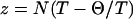(39,40,45). Here, T is the desired temperature and Θ is the theta temperature, where polymers behave like ideal chains, and N is the chain length. It is assumed that the chain swells uniformly vis-à-vis its theta state. The use of theories based on perturbations around the Θ state is only valid in the limit T → Θ or small N. For polymers in the EV limit, z → ∞ and Flory's model is not applicable in this regime. As a consequence, several special characteristics of conformational ensembles for polymers in the EV limit—and, by extension, of highly denatured proteins—are not anticipated by Flory's theory. This observation is not new and several treatises on the subject are available in the polymer literature (39–42).

Departures from Flory's random-coil model are based on field-theoretic approaches (39–42) that explicitly account for the effects of correlations in a self-repelling chain. The goal in these theories is to explain why chain properties such as R_g, R_e, R_h, Π, B₂, scattering functions, and internal correlations obey nontrivial power laws in the EV limit (39). Interestingly, the scaling exponent ν ≈ 0.59 features prominently in all of these power laws. An important prediction of field theory is that all power laws are the result of correlations imparted by repulsive, steric (EV) interactions. The effects of these correlations are present on all length scales. Consequently, in the EV limit, a range of chain properties show so-called scale invariance. Simply stated, chain properties for long chains can be predicted by scaling the corresponding properties for short chains and vice versa. It is on the basis of this invariance to “spatial dilatations” (39) that polymers in the EV limit are said to be renormalizable entities. The availability of an accurate theoretical framework for explaining scale-invariant properties of polymers in the EV limit has important ramifications for developing accurate theoretical descriptions for denatured proteins.

As for specific predictions, a polymer in the EV limit is best described in terms of two distinct length scales (39). All sequence-specific effects are restricted to a single local length scale, denoted as l_s. If one were to examine chain properties at length scales that go above l_s, properties of denatured proteins for different sequences should become indistinguishable from each other. Scale invariance applies to a variety of chain properties that go beyond chain size (39). In the EV limit, the average shape of the chain should be that of a prolate ellipsoid. Internal distances between residues that are beyond l_s should show the same power law dependence on sequence separation as does R_g (or R_e) on chain length (N). The average volume occupied by the chain will be filled inefficiently, and cavities of all sizes l > l_s should be found readily within the interior of a denatured protein. Finally, the ensemble-averaged topology should be invariant with sequence or chain length and the chain is best described as a fractal object of dimension 1.7 (38–40).

In this work, we show that we can simulate conformational ensembles, with atomistic detail, such that ensemble characteristics match the predictions for polymers in the EV limit. We demonstrate this by comparing static, equilibrium properties of the simulated ensembles to those predicted by rigorous field theories. The development of an accurate EV limit description for denatured proteins mirrors the use of the hard-sphere fluid as a reference state for van der Waals liquids (51,52).

Our presentation is organized as follows. First, we present a detailed description of the methods used in our work. Next, we describe six major results to show that characteristics of the simulated EV-limit ensembles are in accord with the predictions of field theories and hence inconsistent with Flory's random coil model. Finally, in the discussion section, we place our results in the context of ongoing debates regarding denatured-state ensembles.

MATERIALS AND METHODS

Potential functions

In the EV limit only the effects of steric interactions are considered. Accordingly, interatomic interactions were modeled using purely repulsive, inverse power potentials (48,53). In our formalism, distinct conformations are specified by a unique set of backbone and side-chain torsion angles, viz., φ, ψ, and χ. The inverse power potential energy (U) for a given conformation is a sum of pairwise interactions. The sum, which runs over all nonbonded pairs of atoms, is written as

(1)

In Eq. 1, σ_ij is the hard-sphere contact distance (54), r_ij is the interatomic separation, and the dispersion parameters ɛ_ij are determined by static polarizability values for individual atoms (55,56).

The values we use for σ_ij and ɛ_ij have been published previously (48). The parameters were chosen to reproduce heats-of-fusion data for model compounds (55). In our EV model, there is only one free parameter, namely the exponent n. For n → ∞, the formula in Eq. 1 resembles the traditional hard-sphere potential (57). For small n, we obtain softer repulsive potentials. A twofold advantage underlies our choice of soft-core repulsions. First, small values of n lend robustness in that our results do not become overly sensitive to the specific choices for values of σ_ij. Second, unlike hard-sphere potentials, which stipulate that all sterically allowed conformations are isoenergetic, soft-core potentials encode the requisite conformational specificity (48,53,58). This has been demonstrated by the generation of quantitative conformational propensities for a range of peptide sequences (48). In this work, we set n = 14. This choice is based on previous work (48), where we showed that conformational propensities for a series of host-guest peptides are insensitive to the choice for n so long as it is in the range n = 9–25.

Degrees of freedom

Bond lengths and bond angles are fixed at equilibrium values taken from the work of Engh and Huber (59). The peptide unit is always trans with ω = 179.5°. The degrees of freedom in all of our calculations are the backbone φ,ψ, and side-chain χ-angles. All sequences are acetylated and N-methylamidated at the N- and C-termini, respectively. If the EV interactions, shown in Eq. 1, are turned off, we obtain Flory's freely rotating chain model (43), albeit with a constraint that the peptide units are all in a trans configuration.

Generation of conformational ensembles

We have adapted conventional Markov-chain Metropolis Monte Carlo simulation strategies (60,61) to generate equilibrium ensembles for each of the protein sequences in the EV limit. Our algorithm is as follows:

1. For a given sequence, N residues long, we start with a random, sterically allowed conformation for the chain and calculate the inverse power potential energy U according to the formula shown in Eq. 1.

2. We then “roll an N-sided die” to choose a residue whose torsion angles are to be altered.

3. We then “flip a two-sided coin” to decide if the trial move is going to be a backbone or side-chain move.

4. Depending on the choice in step 3, the backbone φ,ψ, or side-chain torsions are set to random values in the interval [−180°,180°]. Trial moves that set backbone torsions are pivot moves because these lead to large-scale conformational changes. Conversely, side-chain moves lead to local conformational changes. The proposed torsions are used to compute new Cartesian coordinates for the molecule.

5. Given a new set of Cartesian coordinates from step 4, we calculate the energy for the new conformation. This is referred to as U′. The energy difference ΔU = U – U′ is evaluated. This energy difference is used with the Metropolis criterion (61) to accept or reject the proposed move. In detail, if ΔU < 0, the proposed move is accepted. Alternatively, if ΔU > 0, and a random number that is drawn from the interval [0,1] is less than exp[−βΔU], the proposed move is accepted. For all other cases, the move is rejected. Here, β = 1/RT, where R = 0.00199 kcal/mol-K is the ideal gas constant and T = 298 K is the simulation temperature. If the move is accepted, we set U = U′, return to step 2, and iterate until convergence.

In the algorithm described above, steps 2–5 constitute a single trial move. For a given amino acid sequence, a complete simulation consists of 10⁷ trial moves. For the longest sequence in our data set—the sequence of villin—for which N = 126, generation of the desired conformational ensemble takes ∼20 h on a single 2.4-GHz Intel Xeon processor. Snapshots were saved for analysis once every 10³ trial moves. As a result, for each sequence, we generated an ensemble consisting of 10⁴ uncorrelated conformations. The large-scale motion generated by backbone pivot moves ensures a lack of correlation between saved snapshots.

For each of the amino acid sequences shown in Table 1, ensemble averages and conformational distributions were obtained from an ensemble with a sample size of 10⁴ and the ensembles were generated as discussed above. We have carried out a systematic analysis to assess the quality of data obtained using the protocol described above. Details of these tests for convergence of the simulations and the sample size are presented in the Appendix.

TABLE 1.

Protein sequences for which ensembles in the EV limit were generated^*

Protein Data Bank ID	No. residues	Name	Rg, EV limit (Å)
2PDD	43	PSBD	21.8 ± 0.1
1CQU	56	N-terminal L9	27.1 ± 0.2
3GB1	56	Protein G	26.6 ± 0.1
1SHF:A	59	fyn SH3	27.5 ± 0.2
1CIS	66	CI-2	30.6 ± 0.2
1CSP	67	CspB	29.0 ± 0.2
2HQI	72	MerP	30.7 ± 0.2
1UBQ	76	Ubiquitin	33.5 ± 0.2
2PTL	78	Protein L	32.6 ± 0.3
1PBA	81	ADA2h	34.8 ± 0.3
1HDN	85	HPr	34.8 ± 0.2
1IMQ	86	Im9	35.5 ± 0.2
2ABD	86	ACBP	35.0 ± 0.2
1TEN	90	TnFNIII	36.6 ± 0.3
1LMB:3	92	lambda repressor	36.9 ± 0.3
1WIT	93	Twitchin	37.7 ± 0.3
1URN:A	97	U1A	38.3 ± 0.3
1APS	98	mAcP	38.2 ± 0.3
1TIT	98	titin, 127	38.4 ± 0.3
1HRC	104	Cytochrome c†	39.7 ± 0.3
1APC	106	Cytochrome b562	40.2 ± 0.3
1FKB	107	FKBP	40.3 ± 0.3
2VIK	126	Villin	45.2 ± 0.4

^*Taken from a list of single domain, two state folders (68).

^†The heme group was not included in our calculations. Only the primary sequence information of cytochrome c was used.

The major bottleneck to overcome in the design of efficient Monte Carlo simulations is the O(N²) complexity associated with computing energies for each new conformation. To speed up these calculations, we take advantage of the short range of inverse power potentials (53). Specifically, we ignored the interactions between atoms in residues whose C_α-C_α distance exceeds 15 Å because the inverse power potential energy for these distances is nearly zero. In addition, a 10-Å distance-based cutoff was applied between all nonbonded atoms. We have compared our results to those from previous work (48,58) where no cutoffs were used. We were unable to find any statistically significant differences between results with and without cutoffs. This is mainly because of the short spatial range of EV interactions.

CALCULATION OF SCATTERING PROFILES

The scattering form factor P(q) for a single chain conformation as a function of scattering wave number q is calculated as (62–64)

(2)

In Eq. 2, N is the number of residues, and R_ij is the distance between atoms i and j. To calculate the form factor we used the positions of α-carbon atoms for each residue. For each amino acid sequence, the form factor was calculated for each snapshot generated from the Monte Carlo simulations. The ensemble-averaged form factor, i.e., the average over all 10⁴ conformations, was used to compute the average Kratky profile. The wave numbers used in the calculations range from q = 0 to q = 0.5 Å⁻¹.

Calculation of shape parameters

The shape of a polymer can be quantified in terms of eigenvalues of the radius of gyration tensor. These eigenvalues tell us if a protein in a specific conformation is akin to a sphere, an ellipsoid, or a rod, and, if the polymer is ellipsoidal, is it a prolate or an oblate ellipsoid? We quantify polymer shapes in terms of two parameters, viz., asphericity (δ) and a shape parameter, S. The former quantifies the degree of sphericity and the latter quantifies the principle axis direction in which the deviation from spherical geometry occurs. We follow the prescription of Schäfer (39) and Steinhauser (65) to calculate δ and that of Dima and Thirumalai (66) to calculate S. First, we define the radius of gyration tensor T, compute the eigenvalues of this tensor, and use these eigenvalues to compute δ and S. The prescription is as follows:

(3)

In Eq. 3, λ_i (i = 1, 2, 3) denote eigenvalues of the radius of gyration tensor, T, for a specific conformation. The tensor is computed for each conformation in the ensemble and then diagonalized. The ensemble average in Eq. 3 is computed as an average over all 10⁴ snapshots. For a given conformation in the ensemble, the gyration tensor is computed as

(4)

In Eq. 4, s_i = (r_i – r_CM), where r_CM is the position vector of the center of mass and r_i denotes the position vector of the α-carbon for residue i. The gyration tensor is computed as an outer product of the radius of gyration vector.

RESULTS

In this work, we focus on two-state proteins because the hypothesis is that only two well-defined macrostates— native and highly denatured states—are accessible to these systems (67–70). The underlying assumption is that the highly denatured-state ensemble for two-state proteins can be mimicked using our EV model. Table 1 lists relevant information for the 23 protein sequences (68) used in this study. For each of the sequences shown in Table 1, we used Metropolis Monte Carlo simulations to generate representative conformational ensembles in the EV limit.

Identification of distinct length scales

SAXS (62,63) and small-angle neutron scattering (64) measurements are useful for quantifying the average sizes, shapes, packing densities, and presence of distinct length scales in polymeric solutions. The form factor p(q) or its close counterpart, the Kratky profile (64), q²p(q), provides average structural information across a range of wavelengths. Here, q is in units of inverse wavelength. For each of the sequences shown in Table 1, we computed an ensemble-averaged Kratky profile. The results are shown in Fig. 1. The Kratky profiles reveal the presence of three distinct regimes for each sequence. The first regime 0 ≤ q < 0.08 is the long wavelength regime typically used to quantify the average molecular weight of the polymer. The second, intermediate q regime lies in the interval 0.08 ≤ q < 0.25. The high q regime corresponds to q > 0.25.

FIGURE 1.

Kratky profiles for each of the 23 protein sequences calculated using EV-limit ensembles.

The intermediate and high q regimes provide the most information regarding average chain shape and fluctuations (62–64). Inspection of Kratky profiles in these two regimes suggests the following: in the EV limit, there are two discernible length scales. All sequence-specificity is localized to the high-q, short-wavelength regime. The implication is that sequence specificity influences local rather than nonlocal conformational preferences. In the intermediate q regime, proteins in the EV limit show scale-invariant, sequence-independent behavior wherein properties such as chain size and internal distances follow well-defined power laws.

Kratky profiles for proteins in the EV limit were compared to those of folded proteins and ideal, freely rotating chains (43). An example of this comparison is shown in Fig. 2 for the protein ubiquitin. In the following sections, we show that the differences in Kratky profiles imply that in the EV limit proteins are cigar-shaped, loosely packed coils, with average topologies that are independent of amino acid sequence.

FIGURE 2.

Comparison of Kratky profiles for three different models of ubiquitin, namely, the EV-limit ensemble (dashed curve), the freely rotating chain ensemble (solid curve), and the native structure (dash-dotted curve).

The average shape of a denatured protein is that of a prolate ellipsoid

We computed the ensemble-averaged asphericity values for each of the 23 sequences in the EV limit and the resultant data are shown as cross marks in Fig. 3. For comparison, the δ values calculated from native structures are also shown as open circles. The average asphericity value of 0.5 is independent of sequence in the EV limit. This suggests that proteins in the EV limit have an average ellipsoidal shape. In addition to the asphericity, we computed ensemble-averaged shape parameters (S) for each protein sequence. Again, S = 0 for a perfect sphere. If S < 0, the object is oblate and if S > 0, the object is prolate. The data show that S ≈ 0.7 for all 23 sequences in the EV limit (Fig. 3). The conclusion is that in the EV limit, the average shape for a protein is that of a prolate ellipsoid, i.e., a cigar-shaped object.

FIGURE 3.

Ensemble-averaged asphericity (δ) and shape (S) parameters for all 23 sequences in the EV limit (shown by cross marks) and for folded proteins (open circles). Error bars quantify the standard error in estimation of the mean.

Interestingly, although the average shape is independent of sequence in the EV limit, it clearly depends on sequence for folded proteins. A comparison of the δ and S values of proteins in the EV limit to those of folded proteins is shown in Fig. 3. Although R_g scales with chain length as N^0.34 for folded proteins (66), the scaling law itself does not restrict folded proteins to be spherical globules. This point has been made recently by Dima and Thirumalai (66) who carried out a systematic study of asymmetry in the shapes of folded proteins.

Although the average shape in the EV limit is that of a prolate ellipsoid, the fluctuations in the R_g and δ-values are large. This is shown in Fig. 4 using a contour plot of the two-dimensional distribution function ρ(R_g/N^0.6, δ) for Fyn SH3 domain. The oblong shape reflects the coupling between shape and size. It is also seen that fluctuations span the spectrum of shapes and sizes. In other words, chains in the EV limit are not hard, prolate ellipsoids. Instead, they are soft ellipsoids that show large correlated fluctuations about mean values for R_g and δ. In Fig. 5, we show backbone traces of 10 EV limit conformations each for four different protein sequences. The conformations, which are drawn at random from the ensembles, are oriented in the principle axis frames to illustrate the average prolate ellipsoidal shape as well as the large fluctuations that characterize the conformational distributions.

FIGURE 4.

Two-dimensional probability density plot, ρ(R_g/N^0.6,δ), for the Fyn SH3 domain in the EV limit. The contour plot demonstrates the large fluctuations around the average shape and size that are to be expected in the EV limit.

FIGURE 5.

Ten representative conformations drawn from the EV-limit ensembles for four different protein sequences. The conformations are oriented in the principle axis frame, shown in the bottom left corner for each protein. The snapshots demonstrate both the average prolate shape and the large fluctuations.

Internal correlations show scale invariance

As noted in the introduction, the self-repelling nature of proteins in the EV limit imposes correlations on all length scales. These correlations lead to scale invariance in a variety of chain properties and direct evidence for correlations can be obtained by quantifying the scaling of internal distances. Theory predicts that ensemble-averaged internal distances will scale like ensemble-averaged end-to-end distances such that (39). Here, is the mean-squared end-to-end distance, 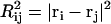, and we choose r_i and r_j to be the position vectors of α-carbon atoms of residues i and j, respectively. The implication is that 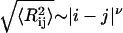, where ν ≈ 0.59. This behavior is expected to hold for all |i − j| > n_s, where n_s denotes the number of residues over which sequence context is important. Predictions for the scaling of internal distances are important because they also allow us to make direct contact with measurements of internal distances in denatured proteins. These measurements are becoming accessible to a variety of experiments that are based on the use of spin labels (71–77).

In Fig. 6, we plot ln(〈R_ij〉) versus ln(|j − i|) for four representative sequences drawn from Table 1. Two parametric lines are used to calibrate the results. The solid lines have slopes of 0.59 and intercepts of 2.0, whereas the dashed lines have slopes of 1.0 and intercepts of 1.335. The latter were derived by assuming a fully extended, rodlike chain with distances between adjacent α-carbon atoms of 3.8 Å. Partial motivation for this reference line comes from the work of Zagrovic and Pande (78), who showed that internal distances in unfolded ensembles of several proteins follow the predictions of the ideal random-flight chain with link length of 3.8 Å. In the EV limit, we find that irrespective of amino acid sequence, internal distances follow the power law predicted by theory for chains in a good solvent. Deviations from the power-law scaling occur for internal distances between residues that are <7 residues apart in sequence.

FIGURE 6.

Scaling of internal distances as a function of sequence separation. Internal correlations are shown for four representative protein sequences. In each of the log-log plots, the solid line has a slope of 0.59 and intercept of 2.0 and the dashed line has a slope of 1.0 and intercept of 1.33. Average internal distances obey the universal power law scaling for sequence separations that go beyond five to nine residues.

For proteins in the EV limit, there are two distinct length scales. The first is a local length scale that spans seven-residue stretches. For sequence separations that go beyond this local length scale, chain properties such as R_g, R_e, and internal distances scale with sequence separation according to universal power laws. Local stiffness is typically quantified in terms of a persistence length, which is the length scale over which the chain behaves like a rigid rod (40,79). The value of R_o obtained from fits to SAXS data for denatured proteins suggests that denatured proteins show rodlike behavior over very short length scales (11). This is also confirmed from our analysis in Fig. 6, which shows that deviations from rodlike behavior occur for all sequence separations greater than a single residue.

Fig. 6 also shows that there is a local length scale over which proteins in the EV limit show nonuniversal behavior. This is not a persistence length. Instead, it is the length scale over which sequence-specific spatial correlations decay. To estimate this length scale, referred to as n_s, we follow the prescription of Thirumalai and Ha (79). Let l_i and l_j be two “bond” vectors. The vector l_i straddles residue i extending between the backbone nitrogen and carbonyl carbon atoms of residue i; the vector l_j straddles residue j. Correlation between a pair of “bond” vectors is quantified by computing the projection, cos(θ_ij), between the vectors. The value for n_s is estimated from a plot of the ensemble average of as a function of , where the latter refers to the sequence separation. If a pair of bonds are highly correlated in the ensemble, then . This is obviously true of adjacent vectors. As the sequence separation increases, the correlations decay, and the value of for which 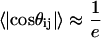is the estimated value for n_s. Fig. 7 shows the calculated values of n_s for all 23 sequences shown in Table 1. Values for n_s range from six to nine residues and do not vary dramatically with protein sequence or chain length. The estimates for n_s appear to be consistent with those from different measurements (80–84) and calculations (48,85). The calculated value of n_s is largest for CI2 and smallest for cold shock protein. It is important to reiterate that the concept of a persistence length is ill defined for a highly flexible chain. It is erroneous to multiply n_s by 3.6 Å (the rise per residue for a fully extended conformation) and stipulate that this is the persistence length for a chain in the EV limit. In fact, the persistence length in the EV limit—the length over which the chain behaves like a straight segment—is <4 Å, i.e., no more than one residue. This estimate agrees with SAXS data, recent atomic force microscopy measurements (86), and simulation results for different proteins (78).

FIGURE 7.

Variation of n_s with sequence for 23 two-state proteins. The top panel shows the ensemble-averaged values of n_s and the bottom panel shows how we estimate n_s from a plot of 〈cos(θ_ij)〉 versus |j − i|, the sequence separation.

Protein interiors in the EV limit reveal cavities on all length scales

Field theories predict that chains in the EV limit are characterized by interior cavities of all sizes, reflecting the inefficient way in which the chains fill the available volume (39). This is a result of correlations that exist on all length scales and the fact that interactions that give rise to these correlations are purely repulsive in nature.

Fig. 8 shows results from our quantitative analysis of cavity statistics for the EV-limit ensembles of proteins. In the interest of clarity, we show data for the sequence of ubiquitin. Similar results were obtained for all other two-state protein sequences shown in Table 1. The question we ask is, what is the probability that a sphere of radius a placed at random with respect to the center of mass of the chain will be empty? For each conformation in the EV-limit ensemble, we place a probe sphere of radius a at several random locations with respect to the center of mass and quantify the number of times a chain atom crosses the probe sphere. This procedure is repeated for all conformations within the ensemble. The resultant data are used to compute P_oa(r), which is defined as the probability of finding a cavity of radius a at a distance r from the center of mass in the ensemble.

FIGURE 8.

Analysis of cavity statistics. This is plotted as the probability P_oa(r) of finding a cavity of size a at a distance r from the center of mass. The data in all of the panels are for the sequence of ubiquitin. (A) EV-limit ensemble of ubiquitin. (B) Folded structure of ubiquitin. (C) Ubiquitin modeled as a fully extended conformation. (D) An ensemble of ubiquitin modeled as a freely rotating chain.

For ubiquitin, we computed P_oa(r) for probe spheres of radii ranging from 2.5 to 12.5 Å. The results are shown in Fig. 8 A. Remarkably, there is a 20% chance of finding a cavity of radius a = 12.5 Å at the average location of the center of mass. The finite probability of finding large cavities within the interior of denatured proteins emphasizes two points: First, the volume occupied by a chain is filled inefficiently when compared to either a folded protein or a freely rotating chain. Second, the cavity statistics are indicative of large-scale correlated fluctuations, which exist on all length scales in the EV limit. To illustrate these points, we compare the values of P_oa(r) obtained in the EV limit to those for three different models.

Cavity statistics, P_oa(r), for folded ubiquitin are shown in Fig. 8 B. In the folded form, the average packing density is high and protein interiors are thought to be either solidlike (87,88) or like “randomly packed spheres near their percolation threshold” (89). Either way, the thinking is that it ought to be difficult to locate spherical cavities of different sizes within protein interiors. Fig. 8 B shows that it is in fact impossible to find room for small or large cavities unless the cavity is located sufficiently far from the center of mass of the folded protein. Interestingly, similar results are obtained for the protein modeled as a fully extended conformation (Fig. 8 C). This erroneous model is of interest only because it has been used previously for denatured proteins in studies aimed at correlating m values and ΔC_P to changes in solvent-accessible surface area (90). In the fully extended conformation, the chain is loosely packed because it is maximally stretched. Yet the probe sphere always intersects the chain unless it is centered sufficiently far away from the center of mass. The results in Fig. 8, B and C, underscore the importance of conformational fluctuations. It is impossible to capture the features of an ensemble, such as the creation of interior cavities, using a single conformation. Comparison of results in Fig. 8 A to those in Fig. 8 C suggest that the “observed” correlation between m values and ΔC_P to changes in solvent-accessible surface area might in fact be serendipitous. A first-principles reassessment of the source of this empirical correlation is mandated. This is the topic of ongoing studies (H. T. Tran and R. V. Pappu, unpublished).

Are fluctuations in the EV limit correlated?

Theory predicts that the gross inefficiency with which the available volume is filled by polymers in the EV limit is in fact a manifestation of correlations between large-scale fluctuations. That this is indeed the case is shown by comparing cavity statistics in the EV limit to values obtained for freely rotating chains. The latter is a model for a soft, Gaussian coil with large-scale, albeit uncorrelated, fluctuations (43). Results for ubiquitin modeled as a freely rotating chain are shown in Fig. 8 D. Since conformational fluctuations are uncorrelated in a chain devoid of interactions, it is impossible to find large cavities (a > 5 Å) within the interior of a freely rotating chain. There is, however, a finite probability of finding small cavities (a < 5 Å) within the interior of a freely rotating chain. In our implementation of the freely rotating chain model, all nonbonded interatomic interactions were turned off and ensembles were generated by drawing the φ,ψ,χ angles for each residue from sterically allowed regions. To implement the true spirit of a Flory model, we could have selected only those conformations that lead to reproduction of the N^0.59 scaling law. Although such an exercise yields higher probabilities for large cavities, the difference is purely qualitative and does not alter the main conclusion.

A summary of the difference between correlated fluctuations in the EV limit and uncorrelated fluctuations for a Flory-like freely rotating chain is shown in Fig. 9, which plots the probabilities, P_oa(r = 0), of finding cavities of different sizes at the ensemble-averaged center-of-mass as a function of cavity radius a. Although P_oa(r = 0) decreases linearly with cavity size, a, for the EV limit, it decays much more rapidly for the freely rotating chain version of ubiquitin. Of course, what we refer to as cavities will actually be filled by solvent and cosolute molecules under denaturing conditions. The main point of the foregoing discussion is that inasmuch as there is congruence between the EV-limit ensemble and highly denatured states, chain fluctuations create ample room to accommodate favorable interactions with the surrounding solvent. Standard reference models such as the fully extended chain and the Flory random coil model will grossly underestimate both the diversity and extent of chain-solvent interactions, which in turn leads to a misrepresentation of the extent and type of conformational fluctuations.

FIGURE 9.

Comparison of the effect of correlated versus of uncorrelated fluctuations on cavity statistics. Here we plot the probability, P_oa(r = 0) of finding a cavity of radius a at the center of mass as a function of cavity radius a. The dashed curve is for the ensemble of ubiquitin modeled as a freely rotating chain (uncorrelated fluctuations) and the solid curve is for the EV-limit ensemble of ubiquitin (correlated fluctuations).

Can the differences quantified in Fig. 8 be tested experimentally?

Fluctuations for a chain of length N will lead to cavities that are large enough to allow for the free diffusion of a smaller chain of length n < N. This observation led Khokhlov and coworkers (91,92) to propose an experiment whereby a reactive group is placed at the center of a chain molecule and the rate of interpolymer reactions is followed as a function of chain length. Reaction rates will be dictated by the accessibility of the reactive group. If denatured proteins follow the Flory random-coil model, the reaction rates would drop exponentially as chain length increases because the reactive group ought to become increasingly inaccessible due to uncorrelated fluctuations. Conversely, for a chain that follows the predictions of field theories in the EV limit, the reaction rate will decrease as some power law with chain length, and there will be a finite probability of realizing a reaction with the reactive group even for very long chains. Advancements in analytical chemistry and mass spectrometry suggest that Khokhlov's proposal can be tested using novel cross-linking approaches that are being developed for quantitative studies of protein folding (93). Other experimental probes can also be used. The form factor in the high q regime provides a measure of the number of interresidue interactions that can be found within a distance a ∼ q⁻¹ from each other and this will scale as a^1.7 (39). Finally, because of the large cavities created by a chain in the EV limit, it is expected that the second virial coefficient (B₂) for highly denatured proteins will scale with chain length as N^0.59 (39,41).

Contacts are hierarchical and average topologies are independent of sequence

Two residues are said to be in contact if there are at least two atoms (including hydrogen atoms), one from each residue, within a 6-Å distance of each other. The histogram of interresidue contacts can be plotted as a contact density map and the results are shown in the top row of Fig. 10 for three proteins of different lengths. Irrespective of chain length and sequence, the contact densities follow a hierarchical pattern whereby near-neighbor residues have a higher probability of being spatially proximal. The probability of finding a pair of residues in close spatial proximity decreases with increasing sequence separation. If one were to zoom into the contact density map of a long protein such as titin one reproduces the contact density map for a shorter protein such as ubiquitin or peripheral subunit binding domain (PSBD). Conversely, zooming out or scaling up from the contact density map of a short protein like PSBD will yield the contact density maps of longer proteins such as ubiquitin or titin. This scale invariance, referred to as dilatation symmetry (39) is a hallmark of chains in the EV limit and reflects the preservation of the hierarchical nature of contact patterns irrespective of sequence or chain length.

FIGURE 10.

Top row shows the contact density maps for EV-limit ensembles of PSBD, ubiquitin, and titin. The color bar for all three plots is shown on the right. To provide a contrast of the folded state to the EV-limit ensemble, the middle row shows contact maps for native structures of PSBD, ubiquitin, and titin. The bottom row shows how the contact density maps in the EV limit come about. Each panel shows distance distributions for different pairs of residues that have different spacing in sequence space. Distance distributions for residues that are local in sequence space are sharply peaked around close distances, whereas distributions for residues that are far apart in sequence are broad and peaked around large distances. The broad distance distributions for distal residues lead to large-scale fluctuations in the EV limit.

The large-scale fluctuations that give rise to the contact density maps shown in Fig. 10 are best explained in terms of distributions for interatomic distances. In the bottom row of Fig. 10 we show distributions of distances obtained for different pairs of residues in the three proteins: PSBD, ubiquitin, and titin. The distributions of distances are sharply peaked for near-neighbor residues and they become increasingly broad as sequence separation increases. In addition, the distance distributions are peaked at larger distance values as sequence separation increases. This emphasizes three important points regarding protein ensembles in the EV limit: First, the dominant contacts are in fact local. Second, the magnitude of fluctuations in interresidue distances increases with increasing sequence separation. Third, these increased fluctuations could certainly lead to the occasional close approach of distal amino acids. Experiments that only detect close spatial contacts will be interpreted as providing evidence of long-range “residual” structure in the denatured state (94–98). Contrary to interpretations of many such experiments, numerous molecular simulations (7,23,99) and recent single-molecule experiments (75) provide little evidence of long-range residual structure under harshly denaturing conditions. The main conclusion is that analysis of the EV-limit ensembles does not preclude the possibility of occasional close contacts between residues that are distal in sequence. It does, however, predict that these contacts have low probabilities and are sampled in the tails of distance distributions. Conventional NMR experiments based on the nuclear Overhauser effect are incapable of resolving contacts that go beyond 5–7 Å. Hence, one must be cautious in interpreting observations of nuclear Overhauser effects as evidence for residual, long-range structure in highly denatured states.

Dilatation symmetry is preserved for all sequences in the EV limit. Conversely, the contact density maps for the folded versions of different sequences reflect differences in native-state topologies. Given access to contact density maps for the denatured state (EV limit) and contact maps for native states, one can make a qualitative judgment regarding the folding process by computing difference contact density maps between the native and denatured states. These difference maps are shown in Fig. 11. These maps show regions where contacts are either present (strong) or absent (weak) in both the native and denatured states. They also show contacts that are strongly represented in the native state and weak in the denatured state. Regions shaded in black are contacts that are pronounced in the denatured state. From the difference contact maps, we find that upon folding, specific nonnative local contacts have to be broken (weakened) to make native, nonlocal spatial contacts. The number and locations of nonnative local contacts that are to be broken determine the sets of spatial contacts that are formed upon folding.

FIGURE 11.

Difference contact density maps for PSBD, ubiquitin, and titin. Contacts that are either missing or weak in the native state but are present in the EV limit are shown in black in the difference contact maps.

Formally, folding can be viewed as a symmetry-breaking operation wherein the dilatation symmetry characteristic of the denatured-state (EV limit) ensemble is broken by breaking or disrupting the requisite number of nonnative local contacts. If folding were strictly driven by the formation of local contacts (100–102), as in a helix-coil transition, then no nonnative local contacts would have to be broken upon folding. Instead, new local contacts would be added onto those that already exist in the denatured state. However, since folding requires the formation of spatial, long-range contacts, local nonnative contacts have to be broken. How the dilatation symmetry of denatured states is broken under folding conditions will depend on a variety of factors including local biases for turns and short stretches of extended or helical conformations, the drive to sequester hydrophobic amino acids, and the achievement of specificity in side-chain packing (103). These interactions will be determined by the specific sequence or, more precisely, by native-state topology.

The importance of native-state topology for folding is underscored by analysis of the average denatured-state topology. Folding rates for two-state proteins show statistically significant correlation with native-state contact order (104). In their original work, Plaxco et al. (104) ignored denatured-state topologies when quantifying the correlation between native-state topology and folding rates. The strong positive correlation between folding rates and contact order implies that folding rates depend only on the end point, i.e., native-state topology. A similar principle underlies the design of energy landscape theories for folding kinetics that are based on Gō models (105–107). At first glance, these results are surprising since the highly denatured state is the starting point for in vitro folding reactions and yet no consideration of the denatured-state topology is required to account for the folding rates. These results would make sense if denatured-state topologies were equivalent and invariant with sequence.

Indeed, for all 23 sequences in the EV limit we find that the absolute contact orders are independent of sequence. We calculated absolute contact order using the method of Plaxco et al. (104). The sequence independence of absolute contact orders in the EV limit is shown in Fig. 12, which plots the absolute ensemble-averaged, EV-limit contact order for all 23 sequences. For comparison, the absolute contact orders of the native-state counterparts are also shown. Since contact order is well-established as a “single value descriptor of topological complexity” (68), the data in Fig. 12 support the conclusion that EV limit ensembles are topologically equivalent. This equivalence in average topologies of denatured states explains why it has been reasonable to ignore the denatured state when assessing the contribution of topology to folding rates for small two-state proteins.

FIGURE 12.

Absolute contact orders for all 23 sequences in the EV limit (cross marks) and for native structures (open circles). Invariance of contact order with sequence in the EV limit suggests that the average topology does not depend on sequence in the denatured state.

The distribution of end-to-end distances

The distribution of end-to-end distances is a fundamental quantity for comparing predictions of different polymer theories (38–42). If 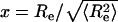, where is the mean-squared end-to-end distance, then is the probability of finding a conformation with x values between x and x + dx. For a Flory random coil, P(x) is a Gaussian distribution of the form . The functional form for P(x) in the EV limit has been derived by des Cloizeaux (41) as an interpolation between the predicted results for P(x) for large (87–110) and small x (111). des Cloizeaux's formula is (41). Here, a_o is a normalization constant, which ensures that .

Fig. 13 shows a comparison of P(x) predicted by theory to distributions computed for four different proteins in the EV limit. Similar data were obtained for all protein sequences shown in Table 1. Simulated data agree with theoretical predictions and the agreement is quantified in terms of residuals between the theoretical distribution and those from simulations. The dashed curve in Fig. 13 is the Gaussian distribution for P(x) that fits a Flory random coil. Comparison of the dashed curve to the other distributions reveals two features of the end-to-end distance distribution in the EV limit. For large x, entropy opposes stretching of the chain beyond its average value of R_e. However, there is a diminution in the entropy in the EV limit vis-à-vis the the Flory model. This is evident in the more rapid decay of P(x) for large x in the EV limit. For small x, the discrepancy is even more pronounced. In the EV limit, there exists a so-called “correlation hole” (39). Stated differently, correlated chain repulsions drastically reduce the probability that the N- and C-termini come very close together. Conversely, P(x) is maximal for small x if one assumes a Flory-style random coil model with uncorrelated fluctuations and uniform (mean-field) chain swelling.

FIGURE 13.

End-to-end distance distribution for five representative sequences in the EV limit. The parameter . The solid curve shows the distribution predicted by des Cloizeaux and the dashed curve is the Gaussian distribution that applies for the Flory random coil. The bottom panel shows residuals between data from EV-limit simulations and the theoretical (solid) curve.

The existence of a correlation hole in the EV limit has been demonstrated in Monte Carlo simulations for a variety of polymeric systems (112,113). Recently, Zhou (114) computed the functional form of x²P(x) from EV simulations of proteins studied by Wilkins et al. (46). The fit obtained by Zhou for x²P(x) (114) is consistent with predictions made by field theory, although Zhou has pursued an alternative interpretation (114–116) of the des Cloizeaux functional form. His interpretation is anchored in refinements (45) of the Flory random coil model (44). Refinements of Flory's mean-field theory have to be used with caution and tailored for each application because they are not designed to capture renormalizable features of polymers in the EV limit (38).

CONCLUSIONS

We have used an atomistic EV model, developed in previous work, to show that it is computationally tractable to generate accurate conformational ensembles for proteins in the EV limit. The accuracy of these ensembles is judged by matching the structural characteristics of the simulated ensembles to those predicted by field theories. Given the equivalence between the EV limit and highly denatured states, our ability to simulate conformational ensembles in the EV limit, with full atomic detail, has direct bearing on the development of an accurate physical picture of conformations accessible to denatured proteins. A summary of our results from analysis of EV-limit ensembles for 23 different two-state proteins is provided below:

1. The average shapes of proteins in the EV limit are akin to those of prolate ellipsoids. This feature is shared with Gaussian chains (39), although clear differences exist in the magnitude of and correlation between conformational fluctuations.

2. We have shown that there are two distinct length scales for proteins in the EV limit. A local length scale spans five- to nine-residue stretches over which sequence-specific spatial correlations decay. Beyond this length scale, all internal distances scale with sequence separation in accordance with the standard power law for proteins in a good solvent.

3. Correlated fluctuations give rise to ensembles that are characterized by a range of internal cavities. The ease of cavitation within the interior of a protein provides a direct measure of the degree of preference for chain-solvent interactions in a perfect solvent.

4. The average topology in the EV limit is independent of amino acid sequence. As a consequence, the EV limit is characterized by hierarchical contacts whereby the distribution of distances between near-neighbor residues is narrow and peaked around smaller values. Conversely, distance distributions for residues that are farther in sequence tend to be broad and peaked at large distances. These hierarchical distance distributions reflect the so-called dilatation symmetry in the EV limit whereby contact density maps for one protein sequence can be rescaled to obtain the contact density map for another sequence.

5. Analysis of difference contact maps suggests that to fold, the dilatation symmetry in the EV limit is broken by weakening specific nonnative local contacts. Precisely how many and which nonnative local contacts are to be broken is determined by the native-state topology and hence the specific amino acid sequence. In other words, although sequence specificity is not apparent in the average denatured-state topology, it is apparent in the way the symmetry characteristic of the denatured state is broken. We believe that this result provides a physical basis for the robustness of native-state topology in protein-folding studies.

6. The distribution of end-to-end distances reveals the presence of a “correlation hole” as was first predicted by des Cloizeaux (41,111) and captures the diminution of entropy vis-à-vis the Flory random-coil estimates. We note that theory also predicts that the number of self-avoiding walks in the EV limit will grow as N^1/6 with chain length N (41,42). We are developing methods to quantify the growth in the size of conformational space with chain length to test this prediction from scaling theories.

Implications for denatured-state ensembles in strongly denaturing environments

Our results have direct bearing on the development of accurate reference-state descriptions for highly denatured proteins. Our efforts based on use of the EV limit mirror the use of the hard-sphere fluid as a reference state for van der Waals liquids (51,52). The ability to simulate denatured-state ensembles is important for a range of applications including protein design (25,26), calculation of stability profiles, understanding the contribution of the denatured state to Φ-values used to quantify structure in the transition state ensembles (117,118), the development of a robust understanding of preferential interactions in cosolute mixtures (31–36), quantifying the interactions between unfolded molecules at high concentrations (29), assessing the presence of residual interactions between hydrophobic as well as charged groups (119–122).

Our ability to simulate mimics of denatured-state ensembles will allow us to ask precise questions about the role of the denatured state in the types of applications outlined above. Of particular interest is the question of how preferential interactions in 8 M urea or 6 M GdnCl conspire to make these conditions mimic perfect solvents for proteins. The recent work of Rösgen et al. (35) suggests that urea, which is chemically equivalent to the main repeating unit in the peptide backbone, can be thought of as a near-perfect solute over the entire solubility range. These observations provide the necessary impetus for developing an accurate statistical thermodynamics framework for understanding how polypeptides respond to increasing concentrations of denaturants to yield ensembles that converge upon the EV limit description.

Our efforts to develop an accurate EV limit description for the denatured-state ensemble parallels the efforts of the Sosnick (124) and Zhou groups (114). There are two obvious differences between our approaches. These two sets of researchers use either coil library statistics (125) or conformations of residues in loops (114) to model local, sequence-context-dependent conformational preferences. To generate ensembles that are self-avoiding, either build-up procedures that screen for long-range hard-sphere steric overlap or Monte Carlo simulations are used. Our approach is different because we use a single potential function to capture both local structure and nonlocal fluctuations. We do not expect there to be any major differences between EV-limit ensembles generated using our approach and the methods used by the Zhou and Sosnick groups. Specifically, we believe that ensembles for proteins obtained in the EV limit (48,124–127), will have characteristics that match predictions from field theories.

There have been numerous attempts to develop models for conformations accessible to highly denatured proteins. These models have an ad hoc flavor and are anchored in Flory's random-coil paradigm, where local biases are modeled accurately and long-range interactions are either ignored or modeled using a mean field. This paradigm forms the basis for the use of tri- and pentapeptides, coil libraries (125,128), and fragments excised from structural databases for modeling properties such as solvent-accessible surface areas (129) in the highly denatured state. None of these models can provide an accurate description of conformational ensembles accessible to highly denatured proteins since they explicitly disregard the effects of correlated fluctuations imposed by two-body EV interactions.

At the other end of the spectrum, recent experimental work and some modeling efforts suggest that a new paradigm is in order for denatured-state ensembles (100,101,130). Apparently, highly denatured states are to be viewed as embryos of native states since it is expected that native-like local and/or nonlocal signals are sampled with statistically significant probability in the denatured-state ensemble (10,130,131). Inasmuch as sequence-specific effects are present over five- to nine-residue stretches, it is conceivable that there are native-like local biases as well as default biases for conformations such as polyproline II (48). However, our assessment of contact density maps, difference contact maps, and topological measures clearly indicate that highly denatured states, which are characterized by dilatation symmetry, are topologically distinct vis-à-vis their native-state counterparts. We speculate that under folding conditions, it is the topological distinction between the native and highly denatured states that provides part of the driving force for folding via collapse and symmetry breaking.

Our work also leads to a direct solution to the reconciliation problem of Plaxco and coworkers (11,47,132). They proposed that observations of residual structure need to be reconciled with the good solvent scaling law obeyed by denatured proteins. Analysis of the EV-limit ensembles suggests that the observations of local sequence-specific contacts are not incompatible with the observed power law behavior. In fact, the existence of two distinct length scales is mandated by field theories. For all sequence separations that go beyond ∼7 residues, ensemble-averaged internal distances show the same power law behavior as R_g and R_e. This scaling ensures that claims of persistent, long-range contacts are not predicted by theories for polymers in the EV limit. Therefore, the reconciliation problem is primarily a debate about how experimental data are interpreted.

The Flory random-coil model has been a topic of intense debate with cases being made for and against this mean-field model as an accurate descriptor of denatured states (132–137). Throughout these discussions, advances in polymer theory that provide an appropriate framework for the description of denatured proteins have largely been ignored. Both the Flory random-coil model and field theories agree that all sequence-specific biases are strictly local and that denatured-state ensembles show significant conformational heterogeneity. However, the mean-field Flory random-coil model is not well-suited for explaining the source of scale-invariant behavior of denatured proteins. This is because it is not applicable to describe polymers in the EV limit. This inherent weakness of the Flory mean-field theory also demands extreme caution when extrapolating simulation or experimental results from peptides (10,12,43,58,101,102,129,138) to draw conclusions about denatured proteins. Peptides do not contain information that goes beyond local propensities and these do not provide insights regarding the correlated fluctuations required to explain how scale invariance of structural, colligative, and thermodynamic properties come about.

The main contribution of field theories is the recognition of the special properties of conformational ensembles that are encoded by correlated fluctuations imposed by the self-repelling nature of a polymer in the EV limit. Inasmuch as these theories are applicable to denatured proteins, the current work shows that many of the seemingly paradoxical observations regarding denatured proteins are readily resolved. Theory and simulation are unambiguous that proteins in the EV limit are topologically distinct from their native-state counterparts, have special renormalizable features, and show hierarchical distance distributions. Interpretations suggesting that highly denatured proteins might be embryos of their native-state counterparts must be treated with extreme caution because there is no sound theoretical basis for such proposals.

APPENDIX: TESTS FOR CONVERGENCE OF MONTE CARLO SIMULATIONS

In the protocol prescribed in the Methods section, a complete Monte Carlo simulation involves 10⁷ trial moves. A snapshot is saved once every 10³ moves for a sample size of 10⁴ conformations in the ensemble for each sequence. We wish to test whether the properties calculated using this ensemble are 1), sensitive to the choice of the initial random conformation; and 2), sensitive to the number of uncorrelated conformations generated in the ensemble. For our test case, we used cytochrome c, a 104-amino-acid sequence, which is one of the longer sequences we have used. It should be noted that cytochrome c is modeled without the heme group, i.e., only the primary sequence information is used.

We generated 10 independent ensembles for cytochrome c using a protocol that is identical to that described in the Methods section. For each of the 10 simulations, we used different, randomly chosen, initial conformations. For each simulation we compute ensemble-averaged properties such as R_g and δ. Comparison of the ensemble-averaged values for these global parameters that assess ensemble-averaged size and shape provides an assessment of the convergence of a single simulation. Table 2 shows the ensemble-averaged R_g, δ, and standard deviations obtained for each of the 10 simulations that have the different initial conformations. The results show that irrespective of the starting conformation, we obtain similar values for R_g and δ. Although it may be possible to achieve this convergence inadvertently for the ensemble average of R_g, convergence for both R_g and δ is a stringent test of the quality of simulations.

TABLE 2.

Results from convergence tests for cytochrome c

Run	Initial Rg (Angstroms)	Initial asphericity	〈Rg〉 (Angst.)	Standard deviation Rg†	〈Asphericity〉
Production*	50.3	0.67	39.7 ± 0.3	8.20	0.48 ± 0.01
1	53.4	0.63	38.9 ± 0.4	8.05	0.49 ± 0.01
2	58.1	0.88	39.5 ± 0.3	8.09	0.49 ± 0.01
3	45.3	0.38	39.4 ± 0.3	8.20	0.48 ± 0.01
4	47.2	0.58	38.8 ± 0.3	8.23	0.49 ± 0.01
5	47.3	0.43	39.4 ± 0.3	8.31	0.49 ± 0.01
6	35.6	0.33	39.4 ± 0.3	8.11	0.49 ± 0.01
7	61.4	0.86	39.7 ± 0.3	8.12	0.49 ± 0.01
8	40.0	0.20	39.5 ± 0.3	8.20	0.48 ± 0.01
9	38.6	0.20	39.5 ± 0.4	8.22	0.49 ± 0.01
10	63.4	0.69	39.6 ± 0.3	8.24	0.48 ± 0.01

^*Production indicates that data from this simulation were used in our analysis discussed in the Results section.

^†For each simulation, we obtain an ensemble and hence a distribution of R_g values, P(R_g). Whereas 〈R_g〉 denotes the first moment of this distribution, the standard deviation is the square root of the variance.

To assess the influence of the size of the ensemble (10⁴ per sequence), we concatenated the ensembles from the 10 independent simulations to generate a cumulative ensemble with 10⁵ conformations. Ensemble-averaged R_g and δ values were computed with samples of size varying from 10 to 10⁵. For a sample size that is very small (<10²), the ensemble-averaged values deviate measurably from the mean values. However, for sample sizes >500, convergence of ensemble-averaged values is readily achieved. Data from these analyses are shown in Fig. 14. Based on the foregoing discussion, we conclude that our sampling protocol provides an accurate and converged description of atomic-level spontaneous fluctuations in the EV limit.

FIGURE 14.

Results of convergence tests which show that the use of 10⁴ representative conformations to mimic EV-limit ensembles for each sequence yields converged results for both average radius of gyration (R_g) and asphericity (δ).

References

- 1.Kauzmann, W. 1959. Some factors in the interpretation of protein denaturation. Adv. Protein Chem. 14:1–63. [DOI] [PubMed] [Google Scholar]
- 2.Miller, W. G., and C. V. Goebel. 1968. Dimensions of protein random coils. Biochemistry. 7:3925–3935. [DOI] [PubMed] [Google Scholar]
- 3.Tanford, C. 1968. Protein denaturation. Adv. Protein Chem. 23:121–282. [DOI] [PubMed] [Google Scholar]
- 4.Dill, K. A., and D. Shortle. 1991. Deantured states of proteins. Annu. Rev. Biochem. 60:795–825. [DOI] [PubMed] [Google Scholar]
- 5.Shortle, D. 1996. The denatured state (the other half of the folding equation) and its role in protein stability. FASEB J. 10:27–34. [DOI] [PubMed] [Google Scholar]
- 6.Smith, L. J., K. M. Fiebig, H. Schwalbe, and C. M. Dobson. 1996. The concept of a random coil: residual structure in peptides and denatured proteins. Fold. Des. 1:R95–R106. [DOI] [PubMed] [Google Scholar]
- 7.Wong, K. B., J. Clarke, C. J. Bond, J. L. Neira, S. M. V. Freund, A. R. Fersht, and V. Daggett. 2000. Towards a complete description of the structural and dynamic properties of the denatured state of barnase and the role of residual structure in folding. J. Mol. Biol. 296:1257–1282. [DOI] [PubMed] [Google Scholar]
- 8.van Gunsteren, W. F., R. Burgi, C. Peter, and X. Daura. 2001. The key to solving the protein-folding problem lies in an accurate description of the denatured state. Angew. Chem. Int. Ed. Engl. 40:351–355. [DOI] [PubMed] [Google Scholar]
- 9.Schellman, J. A. 2002. Fifty years of solvent denaturation. Biophys. Chem. 96:91–101. [DOI] [PubMed] [Google Scholar]
- 10.Baldwin, R. L. 2002. A new perspective on unfolded proteins. Adv. Protein Chem. 62:361–367. [DOI] [PubMed] [Google Scholar]
- 11.Kohn, J. E., I. S. Millett, J. Jacob, B. Zagrovic, T. M. Dillon, N. Cingel, R. S. Dothager, S. Seifert, P. Thiyagarajan, T. R. Sosnick, M. Z. Hasan, V. S. Pande, I. Ruzcinski, S. Doniach, and K. W. Plaxco. 2004. Random-coil behavior and the dimensions of chemically unfolded proteins. Proc. Natl. Acad. Sci. USA. 101:12491–12496. [DOI] [PMC free article] [PubMed] [Google Scholar]
- 12.Fleming, P. J., and G. D. Rose. 2005. Conformational properties of unfolded proteins. In Protein Folding Handbook, Vol. 2. J. Buchner and T. Kiefhaber, editors. Wiley-VCH, Weinheim, Germany. 710–736.
- 13.Dill, K. A., and D. Stigter. 1995. Modeling protein stability as heteropolymer collapse. Adv. Protein Chem. 46:59–104. [DOI] [PubMed] [Google Scholar]
- 14.Robertson, A. D., and K. P. Murphy. 1997. Protein structure and the energetics of protein stability. Chem. Rev. 97:1251–1267. [DOI] [PubMed] [Google Scholar]
- 15.Laziridis, T., and M. Karplus. 2003. Thermodynamics of protein folding: a microscopic view. Biophys. Chem. 100:367–395. [DOI] [PubMed] [Google Scholar]
- 16.Garcia-Moreno, B., and C. A. Fitch. 2004. Structural interpretation of pH and salt-dependent processes in proteins with computational methods. Methods Enzymol. 380:20–51. [DOI] [PubMed] [Google Scholar]
- 17.Zhou, H.-X. 2004. Polymer models of protein stability, folding, and interactions. Biochemistry. 43:2141–2154. [DOI] [PubMed] [Google Scholar]
- 18.Pace, C. N., G. R. Grimsley, and J. M. Scholtz. 2005. Denaturant-induced protein unfolding. In Protein Folding Handbook, Vol. 1. J. Buchner and T. Kiefhaber, editors. Wiley-VCH, Weinheim, Germany. 45–69.
- 19.Bryngelson, J. D., J. N. Onuchic, N. D. Socci, and P. G. Wolynes. 1995. Funnels, pathways, and the energy landscape of protein folding: a synthesis. Proteins.. 21:167–195. [DOI] [PubMed] [Google Scholar]
- 20.Dill, K. A., and H. S. Chan. 1997. From Levinthal to pathways to funnels. Nat. Struct. Biol. 4:10–19. [DOI] [PubMed] [Google Scholar]
- 21.Baldwin, R. L., and G. D. Rose. 1999. Is protein folding hierarchic? II. Trends Biochem. Sci. 24:77–83. [DOI] [PubMed] [Google Scholar]
- 22.Dinner, A. R., A. Sali, L. J. Smith, C. M. Dobson, and M. Karplus. 2000. Understanding protein folding via free energy surfaces from theory and experiments. Trends Biochem. Sci. 25:331–339. [DOI] [PubMed] [Google Scholar]
- 23.Daggett, V. 2002. Molecular dynamics simulations of the protein unfolding/folding reaction. Acc. Chem. Res. 35:422–429. [DOI] [PubMed] [Google Scholar]
- 24.Religa, T. L., J. S. Markson, U. Mayor, S. M. V. Freund, and A. R. Fersht. 2005. Solution structure of a protein denatured state and folding intermediate. Nature. 437:1053–1056. [DOI] [PubMed] [Google Scholar]
- 25.Mendes, J., R. Guerois, and L. Serrano. 2002. Energy estimation in protein design. Curr. Opin. Struct. Biol. 12:441–446. [DOI] [PubMed] [Google Scholar]
- 26.Anil, B., R. Craig-Schapiro, and D. P. Raleigh. 2006. Design of a hyperstable protein by rational consideration of unfolded state interactions. J. Am. Chem. Soc. 128:3144–3145. [DOI] [PubMed] [Google Scholar]
- 27.Dobson, C. M. 2004. Principles of protein folding, misfolding, and aggregation. Semin. Cell Dev. Biol. 15:3–16. [DOI] [PubMed] [Google Scholar]
- 28.Ohnishi, S., and K. Takano. 2004. Amyloid fibrils from the viewpoint of protein folding. Cell. Mol. Life Sci. 61:511–524. [DOI] [PMC free article] [PubMed] [Google Scholar]
- 29.Uversky, V. N., and A. L. Fink. 2004. Conformational constraints for amyloid formation: the importance of being unfolded. Biochim. Biophys. Acta. 1698:131–153. [DOI] [PubMed] [Google Scholar]
- 30.Tanford, C. 1970. Protein denaturation: C. Theoretical models for the mechanism of denaturation. Adv. Protein Chem. 24:1–95. [PubMed] [Google Scholar]
- 31.Makhatadze, G. I. 1999. Thermodynamics of protein interactions with urea and guanidinium hydrochloride. J. Phys. Chem. B. 103:4781–4785. [Google Scholar]
- 32.Schellman, J. A. 2003. Protein stability in mixed solvents: A balance of contact interactions and excluded volume. Biophys. J. 85:108–125. [DOI] [PMC free article] [PubMed] [Google Scholar]
- 33.Ferreon, A. C. M., and D. W. Bolen. 2004. Thermodynamics of denaturant-induced unfolding of a protein that exhibits variable two-state denaturation. Biochemistry. 43:13357–13369. [DOI] [PubMed] [Google Scholar]
- 34.Felitsky, D. J., and M. T. Record. 2004. Application of the local-bulk partitioning and competitive binding models to interpret preferential interactions of glycine betaine and urea with protein surface. Biochemistry. 43:9276–9288. [DOI] [PubMed] [Google Scholar]
- 35.Rösgen, J., B. M. Pettitt, and D. W. Bolen. 2005. Bolen. Protein folding, stability, and solvation structure in osmolyte solutions. Biophys. J. 89:2988–2997. [DOI] [PMC free article] [PubMed] [Google Scholar]
- 36.Auton, M., and D. W. Bolen. 2005. Predicting the energetics of osmolyte-induced protein folding/unfolding. Proc. Natl. Acad. Sci. USA. 102:15065–15068. [DOI] [PMC free article] [PubMed] [Google Scholar]
- 37.Chan, H. S., and K. A. Dill. 1991. Polymer principles in protein structure and stability. Annu. Rev. Biophys. Biophys. Chem. 20:447–490. [DOI] [PubMed] [Google Scholar]
- 38.Rubenstein, M., and R. H. Colby. 2003. Polymer Physics. Oxford University Press, New York.
- 39.Schäfer, L. 1999. Excluded Volume Effects in Polymer Solutions as Explained by the Renormalization Group. Springer, Berlin.
- 40.Grosberg, A. Y., and A. R. Khokhlov. 1994. Statistical Physics of Macromolecules. AIP Series in Polymers and Complex Materials. American Institute of Physics, New York.
- 41.des Cloizeaux, J., and G. Janink. 1990. Polymers in Solution: Their Modeling and Structure. Oxford University Press, Oxford, UK.
- 42.de Gennes, P. G. 1979. Scaling Concepts in Polymer Physics. Cornell University Press, Ithaca, NY.
- 43.Flory, P. J. 1969. Statistical Mechanics of Chain Molecules. Hanser Publishers, Munich.
- 44.Flory, P. J. 1953. Principles of Polymer Chemistry. Cornell University Press, Ithaca, NY.
- 45.Sanchez, I. C. 1979. Phase transition behavior of the isolated polymer chain. Macromolecules. 12:980–988. [Google Scholar]
- 46.Wilkins, D. K., S. B. Grimshaw, V. Receveur, C. M. Dobson, J. A. Jones, and L. J. Smith. 1999. Hydrodynamic radii of native and denatured proteins measured by pulse field gradient NMR techniques. Biochemistry. 38:16424–16431. [DOI] [PubMed] [Google Scholar]
- 47.Millett, I. S., S. Doniach, and K. W. Plaxco. 2002. Toward a taxonomy of the denatured state: small angle scattering studies of unfolded proteins. Adv. Protein Chem. 62:241–262. [DOI] [PubMed] [Google Scholar]
- 48.Tran, H. T., X. Wang, and R. V. Pappu. 2005. Reconciling sequence-specific conformational preferences with generic behavior of denatured proteins. Biochemistry. 44:11369–11380. [DOI] [PubMed] [Google Scholar]
- 49.Le Guillou, J. C., and J. Zinn-Justin. 1980. Critical exponents from field theory. Phys. Rev. B. 21:3976–3998. [Google Scholar]
- 50.Receveur, V., D. Durand, M. Desmadril, and P. Calmattes. 1998. Repulsive interparticle interactions in a denatured protein solution revealed by small angle neutron scattering. FEBS Lett. 426:57–61. [DOI] [PubMed] [Google Scholar]
- 51.Hansen, J.-P., and I. R. McDonald. 1986. Theory of Simple Liquids. Academic Press, London.
- 52.Chandler, D., J. D. Weeks, and H. C. Andersen. 1983. van der Waals picture of liquids, solids, and phase transformations. Science. 220:787–794. [DOI] [PubMed] [Google Scholar]
- 53.Hoover, W. G., S. G. Gray, and K. W. Johnson. 1971. Thermodynamic properties of the fluid and solid phases for inverse power potentials. J. Chem. Phys. 55:1128–1136. [Google Scholar]
- 54.Hopfinger, A. J. 1973. Conformational Properties of Macromolecules. Academic Press, New York.
- 55.Pauling, L. 1970. General Chemistry, 3rd ed.. W. H. Freeman Press, San Francisco.
- 56.Slater, J. C., and J. G. Kirkwood. 1931. The van der Waals forces in gases. Phys. Rev. 37:682–696. [Google Scholar]
- 57.Stillinger, F. H., and T. A. Weber. 1985. Inherent structure theory of liquids in the hard-sphere limit. J. Chem. Phys. 83:4767–4775. [Google Scholar]
- 58.Pappu, R. V., and G. D. Rose. 2002. A simple model for poly-proline II structure in unfolded states of alanine-based peptides. Protein Sci. 11:2437–2455. [DOI] [PMC free article] [PubMed] [Google Scholar]
- 59.Engh, R. A., and R. Huber. 1991. Accurate bond and angle parameters for X-ray protein structure refinement. Acta Crystallogr. 47:392–400. [Google Scholar]
- 60.Frenkel, D., and B. Smit. 2002. Understanding Molecular Simulation. From Algorithms to Applications. Academic Press, London, UK.
- 61.Metropolis, N., A. W. Rosenbluth, M. N. Rosenbluth, A. H. Teller, and E. Teller. 1953. Equation of state calculations by fast computing machines. J. Chem. Phys. 21:1087–1092. [Google Scholar]
- 62.Glatter, O., and O. Kratky. 1982. Small Angle X-Ray Scattering. Academic Press, London.
- 63.Doniach, S. 2001. Changes in biomolecular conformation seen by small angle X-ray scattering. Chem. Rev. 101:1763–1778. [DOI] [PubMed] [Google Scholar]
- 64.Higgins, J. L., and H. C. Benoit. 1994. Polymers and Neutron Scattering. Oxford Science Publications, Clarendon Press, Oxford.
- 65.Steinhauser, M. O. 2005. A molecular dynamics study on universal properties of polymer chains in different solvent qualities. Part I. A review of linear chain properties. J. Chem. Phys. 122:094901. [DOI] [PubMed] [Google Scholar]
- 66.Dima, R. I., and D. Thirumalai. 2004. Asymmetry in the shapes of folded and denatured states of proteins. J. Phys. Chem. B. 108:6564–6570. [Google Scholar]
- 67.Jackson, S. E. 1998. How to small single-domain proteins fold? Fold. Des. 3:R81–R91. [DOI] [PubMed] [Google Scholar]
- 68.Plaxco, K. W., K. T. Simons, I. Ruczinski, and D. Baker. 2000. Topology, stability, sequence, and length: defining the determinants of two-state protein folding kinetics. Biochemistry. 39:11177–11183. [DOI] [PubMed] [Google Scholar]
- 69.Lumry, R., and R. Biltonen. 1966. Validity of the “two-state” hypothesis for conformational transitions for proteins. Biopolymers. 4:917–944. [DOI] [PubMed] [Google Scholar]
- 70.Jackson, W. M., and J. F. Brandts. 1970. Thermodynamics of protein denaturation. A calorimetric study of the reversible denaturation of chymotrypsinogen and conclusions regarding the validity of the two-state approximation. Biochemistry. 9:2294–2301. [DOI] [PubMed] [Google Scholar]
- 71.Gillespie, J., and D. Shortle. 1997. Characterization of long-range structure in the denatured state of staphylococcal nuclease. 1. Paramagnetic relaxation enhancement by nitroxide spin labels. J. Mol. Biol. 268:158–169. [DOI] [PubMed] [Google Scholar]
- 72.Kristjansdottir, S., K. Lindorff-Larsen, W. Fieber, C. M. Dobson, M. Vendruscolo, and F. M. Poulsen. 2005. Formation of native and non-native interactions in ensembles of ACBP molecules from paramagnetic spin relaxation enhancement studies. J. Mol. Biol. 347:1053–1062. [DOI] [PubMed] [Google Scholar]
- 73.Lindorff-Larsen, K., S. Kristjansdottir, K. Teilum, W. Fieber, C. M. Dobson, F. M. Poulsen, and M. Vendruscolo. 2004. Determination of an ensemble of structures representing the denatured state of the bovine acyl-coenzyme A binding protein. J. Am. Chem. Soc. 126:3291–3299. [DOI] [PubMed] [Google Scholar]
- 74.Chattopadhyay, K., S. Safarian, E. L. Elson, and C. Frieden. 2005. Measuring unfolding of proteins in the presence of denaturant using fluorescence correlation spectroscopy. Biophys. J. 88:1413–1422. [DOI] [PMC free article] [PubMed] [Google Scholar]
- 75.McCarney, E. R., J. H. Werner, S. L. Bernstein, I. Ruczinski, D. E. Makarov, P. M. Goodwin, and K. W. Plaxco. 2005. Site-specific dimensions across a highly denatured protein: A single molecule study. J. Mol. Biol. 352:672–682. [DOI] [PubMed] [Google Scholar]
- 76.Sinha, K. K., and J. B. Udgaonkar. 2005. Dependence of the size of the initially collapsed form during the refolding of barstar on denaturant concentration: Evidence for a continuous transition. J. Mol. Biol. 353:704–718. [DOI] [PubMed] [Google Scholar]
- 77.Bhavesh, N. S., J. Juneja, J. B. Udgaonkar, and R. V. Hosur. 2004. Native and nonnative conformational preferences in the urea-unfolded state of barstar. Protein Sci. 13:3085–3091. [DOI] [PMC free article] [PubMed] [Google Scholar]
- 78.Zagrovic, B., and V. S. Pande. 2003. Structural correspondence between the α-helix and the random-flight chain resolves how unfolded proteins can have native-like properties. Nat. Struct. Biol. 10:955–961. [DOI] [PubMed] [Google Scholar]
- 79.Thirumalai, D., and B.-Y. Ha. 1998. Statistical mechanics of semi-flexible chains: A mean field variational approach. In Theoretical and Mathematical Models in Polymer Research. A. Grosberg, editor. Academic Press, Boston. 1–35.
- 80.Damaschun, G., H. Damaschun, K. Gast, R. Misselwitz, J. J. Muller, W. Pfeil, and D. Zirwer. 1993. Cold denaturation-induced conformational changes in phosphoglycerate kinase from yeast. Biochemistry. 32:7739–7746. [DOI] [PubMed] [Google Scholar]
- 81.Schwalbe, H., K. M. Fiebig, M. Buck, J. A. Jones, S. B. Grimshaw, A. Spencer, S. J. Glaser, L. J. Smith, and C. M. Dobson. 1997. Structural and dynamical properties of a denatured protein. Heteronuclear 3D NMR experiments and theoretical simulations of lysozyme in 8M urea. Biochemistry. 36:8977–8991. [DOI] [PubMed] [Google Scholar]
- 82.Damaschun, G., H. Damaschun, K. Gast, and D. Zirwer. 1999. Proteins can adopt totally different folded conformations. J. Mol. Biol. 291:715–725. [DOI] [PubMed] [Google Scholar]
- 83.Schwarzinger, S., P. E. Wright, and H. J. Dyson. 2002. Molecular hinges in protein folding: The urea-denatured state of apomyoglobin. Biochemistry. 41:12681–12686. [DOI] [PubMed] [Google Scholar]
- 84.Mohana-Borges, R., N. K. Goto, G. J. A. Kroon, H. J. Dyson, and P. E. Wright. 2004. Structural characterization of unfolded states of apomyoglobin using residual dipolar couplings. J. Mol. Biol. 340:1131–1142. [DOI] [PubMed] [Google Scholar]
- 85.Ohkubo, Y. Z., and C. L. Brooks. 2003. Exploring Flory's isolated-pair hypothesis: statistical mechanics of helix-coil transitions in polyalanine and the C-peptide from RNase A. Proc. Natl. Acad. Sci. USA. 100:13916–13921. [DOI] [PMC free article] [PubMed] [Google Scholar]
- 86.Thompson, J. B., H. G. Hansma, P. K. Hansma, and K. W. Plaxco. 2002. The backbone conformational entropy of protein folding: experimental measures from atomic force microscopy. J. Mol. Biol. 322:645–652. [DOI] [PubMed] [Google Scholar]
- 87.Richards, F. M. 1977. Areas, volumes, packing and protein structure. Annu. Rev. Biophys. Bioeng. 6:151–176. [DOI] [PubMed] [Google Scholar]
- 88.Zhou, Y., D. Vitkup, and M. Karplus. 1999. Native proteins are surface-molten solids: application of the Lindemann criterion for the solid versus liquid state. J. Mol. Biol. 285:1371–1375. [DOI] [PubMed] [Google Scholar]
- 89.Liang, J., and K. A. Dill. 2001. Are proteins well packed? Biophys. J. 81:751–766. [DOI] [PMC free article] [PubMed] [Google Scholar]
- 90.Myers, J. K., C. N. Pace, and J. M. Scholtz. 1995. Denaturant m-values and heat capacity changes: relation to changes in accessible surface areas of protein unfolding. Protein Sci. 4:2138–2148. [DOI] [PMC free article] [PubMed] [Google Scholar]
- 91.Khokhlov, A. R. 1981. Influence of excluded volume effect on the rates of polymer-polymer interactions. Macromol. Rapid Commun. 2:633–636. [Google Scholar]
- 92.Grosberg, A. Y., P. G. Khalatur, and A. R. Khokhlov. 1983. Polymer coils with excluded volume in dilute solution: The invalidity of the model of impenetrable spheres and the influence of excluded volume on the rates of diffusion-controlled intermolecular reactions. Macromol. Rapid Commun. 3:709–713. [Google Scholar]
- 93.Leavell, M. D., P. Novak, C. R. Behrens, J. S. Schoeniger, and G. H. Kruppa. 2004. Strategy for selective chemical cross-linking of tyrosine and lysine residues. J. Am. Soc. Mass Spectrom. 15:1604–1611. [DOI] [PubMed] [Google Scholar]
- 94.Ohnishi, S., A. L. Lee, M. H. Edgell, and D. Shortle. 2004. Direct demonstration of structural similarity between native and denatured eglin C. Biochemistry. 43:4064–4070. [DOI] [PubMed] [Google Scholar]
- 95.Ackerman, M. S., and D. Shortle. 2002. Robustness of the long-range structure in denatured staphylococcal nuclease to changes in amino acid sequence. Biochemistry. 41:13791–13797. [DOI] [PubMed] [Google Scholar]
- 96.Hodsdon, M. E., and C. Frieden. 2001. Intestinal fatty acid binding protein: The folding mechanism as determined by NMR studies. Biochemistry. 40:732–742. [DOI] [PubMed] [Google Scholar]
- 97.Klein-Seetharaman, J., M. Oikawa, S. B. Grimshaw, J. Wirmer, E. Duchardt, T. Ueda, T. Imoto, L. J. Smith, C. M. Dobson, and H. Schwalbe. 2002. Long-range interactions within a non-native protein. Science. 295:1719–1722. [DOI] [PubMed] [Google Scholar]
- 98.Koepf, E. K., H. M. Petrassi, M. Sudol, and J. W. Kelly. 1999. An isolated three-stranded antiparallel β-sheet domain that unfolds and refolds reversibly: Evidence for a structured hydrophobic cluster in urea and GdnHCl and a disordered thermal unfolded state. Protein Sci. 8:841–853. [DOI] [PMC free article] [PubMed] [Google Scholar]
- 99.Ferguson, N., R. Day, C. M. Johnson, M. D. Allen, V. Daggett, and A. R. Fersht. 2005. Simulation and experiment at high temperatures: ultrafast folding of a thermophilic protein by nucleation-condensation. J. Mol. Biol. 347:855–870. [DOI] [PubMed] [Google Scholar]
- 100.Fitzkee, N. C., and G. D. Rose. 2004. Reassessing random-coil statistics in unfolded proteins. Proc. Natl. Acad. Sci. USA. 101:12497–12502. [DOI] [PMC free article] [PubMed] [Google Scholar]
- 101.Fitzkee, N. C., and G. D. Rose. 2005. Sterics and solvation winnow accessible conformational space for unfolded proteins. J. Mol. Biol. 353:873–887. [DOI] [PubMed] [Google Scholar]
- 102.Ding, L., K. Chen, P. A. Santini, Z. S. Shi, and N. R. Kallenbach. 2003. The pentapeptide GGAGG has PII conformation. J. Am. Chem. Soc. 125:8092–8093. [DOI] [PubMed] [Google Scholar]
- 103.Li, H., and C. Frieden. 2005. Phenylalanine side chain behavior of the intestinal fatty acid-binding protein: the effect of urea on backbone and side chain stability. J. Biol. Chem. 280:38556–38561. [DOI] [PubMed] [Google Scholar]
- 104.Plaxco, K. W., K. T. Simons, and D. Baker. 1998. Contact order, transition state placement, and the refolding rates of single domain proteins. J. Mol. Biol. 277:985–994. [DOI] [PubMed] [Google Scholar]
- 105.Shea, J.-E., J. N. Onuchic, and C. L. Brooks. 1999. Exploring the origins of topological frustration: design of a minimally frustrated fragment of the B domain of protein A. Proc. Natl. Acad. Sci. USA. 96:12512–12517. [DOI] [PMC free article] [PubMed] [Google Scholar]
- 106.Clementi, C., P. A. Jennings, and J. N. Onuchic. 2000. How native-state topology affects the folding of dihydrofolate reductase and interleukin-1β. Proc. Natl. Acad. Sci. USA. 97:5871–5876. [DOI] [PMC free article] [PubMed] [Google Scholar]
- 107.Go, N. 1983. Theoretical studies of protein folding. Annu. Rev. Biophys. Bioeng. 12:183–210. [DOI] [PubMed] [Google Scholar]
- 108.Fisher, M. E. 1966. Shape of a self-avoiding walk of a polymer chain. J. Chem. Phys. 44:616–622. [Google Scholar]
- 109.McKenzie, D. S., and M. A. Moore. 1971. Shape of a self-avoiding walk or polymer chain. J. Phys. A. Math. Gen. 4:L82–L86. [Google Scholar]
- 110.McKenzie, D. S. 1973. The end-to-end length distribution of self-avoiding walks. J. Phys. A.: Math. Nucl. Gen. 6:338–352. [Google Scholar]
- 111.des Cloizeaux, J. 1974. Lagrangian theory of a self-avoiding random chain. Phys. Rev. A. 10:1665–1669. [Google Scholar]
- 112.Bishop, M., and J. H. R. Clarke. 1991. Investigation of the end-to-end distance distribution function for random and self-avoiding walks in two and three dimensions. J. Chem. Phys. 94:3936–3942. [Google Scholar]
- 113.Valleau, J. P. 1996. Distribution of end-to-end length of an excluded volume chain. J. Chem. Phys. 104:3071–3074. [Google Scholar]
- 114.Zhou, H.-X. 2002. Dimensions of denatured protein chains from hydrodynamic data. J. Phys. Chem. B. 106:5769–5775. [Google Scholar]
- 115.Zhou, H.-X. 2002. A Gaussian-chain model for treating residual charge-charge interactions in the unfolded state of proteins. Proc. Natl. Acad. Sci. USA. 99:3569–3574. [DOI] [PMC free article] [PubMed] [Google Scholar]
- 116.Zhou, H.-X. 2003. Direct test of the Gaussian-chain model for treating residual charge-charge interactions in the unfolded state of proteins. J. Am. Chem. Soc. 125:2060–2061. [DOI] [PubMed] [Google Scholar]
- 117.Brewer, S. H., D. M. Vu, Y. F. Tang, S. Franzen, D. P. Raleigh, and R. B. Dyer. 2005. Effect of modulating unfolded state structure on the folding kinetics of the villin headpiece subdomain. Proc. Natl. Acad. Sci. USA. 102:16662–16667. [DOI] [PMC free article] [PubMed] [Google Scholar]
- 118.Horng, J. C., J. H. Cho, and D. P. Raleigh. 2005. Analysis of pH-dependent folding and stability of histidine point mutants allows characterization of the denatured state and transition state for protein folding. J. Mol. Biol. 345:163–173. [DOI] [PubMed] [Google Scholar]
- 119.Trefethen, J. M., C. N. Pace, J. M. Scholtz, and D. N. Brems. 2005. Charge-charge interactions in the denatured state influence the folding kinetics of ribonuclease Sa. Protein Sci. 14:1934–1938. [DOI] [PMC free article] [PubMed] [Google Scholar]
- 120.Cho, J. H., and D. P. Raleigh. 2005. Mutational analysis demonstrates that specific electrostatic interactions can play a key role in the denatured ensembles of proteins. J. Mol. Biol. 353:174–185. [DOI] [PubMed] [Google Scholar]
- 121.Li, Y., F. Picart, and D. P. Raleigh. 2005. Direct characterization of the folded, unfolded, and urea-denatured states of the C-terminal domain of the ribosomal protein L9. J. Mol. Biol. 349:839–846. [DOI] [PubMed] [Google Scholar]
- 122.Cho, J. H., S. Sato, and D. P. Raleigh. 2004. Thermodynamics and kinetics of non-native interactions in protein folding: a single point mutant significantly stabilizes the N-terminal domain of L9 by modulating non-native interactions in the denatured state. J. Mol. Biol. 338:827–837. [DOI] [PubMed] [Google Scholar]
- 123.Reference deleted in proof.
- 124.Jha, A. K., A. Colubri, K. F. Freed, and T. R. Sosnick. 2005. Statistical coil model of the unfolded state: resolving the reconciliation problem. Proc. Natl. Acad. Sci. USA. 102:13099–13104. [DOI] [PMC free article] [PubMed] [Google Scholar]
- 125.Jha, A. K., A. Colubri, M. H. Zaman, S. Koide, T. R. Sosnick, and K. F. Freed. 2005. Helix, sheet, and polyproline II frequencies and strong nearest neighbor effects in a restricted coil library. Biochemistry. 44:9691–9702. [DOI] [PubMed] [Google Scholar]
- 126.Goldenberg, D. P. 2003. Computational simulation of the statistical properties of unfolded proteins. J. Mol. Biol. 326:1615–1633. [DOI] [PubMed] [Google Scholar]
- 127.Ding, F., R. K. Jha, and N. V. Dokholyan. 2005. Scaling behavior and structure of denatured proteins. Structure. 13:1047–1054. [DOI] [PubMed] [Google Scholar]
- 128.Smith, L. J., K. A. Bolin, H. Schwalbe, M. W. MacArthur, J. M. Thornton, and C. M. Dobson. 1996. Analysis of main chain torsion angles in proteins: prediction of NMR coupling constants for native and random coil conformations. J. Mol. Biol. 255:494–506. [DOI] [PubMed] [Google Scholar]
- 129.Creamer, T. P., R. Srinivasan, and G. D. Rose. 1995. Modeling unfolded proteins of peptides and proteins. Biochemistry. 34:16245–16250. [DOI] [PubMed] [Google Scholar]
- 130.Shortle, D., and M. S. Ackerman. 2001. Persistence of native-like topology in a denatured protein in 8M urea. Science. 293:487–489. [DOI] [PubMed] [Google Scholar]
- 131.Choy, W. Y., and J. D. Forman-Kay. 2001. Calculation of ensembles of structures representing the unfolded state of an SH3 domain. J. Mol. Biol. 308:1011–1032. [DOI] [PubMed] [Google Scholar]
- 132.McCarney, E. R., J. E. Kohn, and K. W. Plaxco. 2005. Is there or isn't there? The case for (and against) residual structure in chemically denatured proteins. Crit. Rev. Biochem. Mol. Biol. 40:181–189. [DOI] [PubMed] [Google Scholar]
- 133.Rose, G. D. Getting to know u. 2002. Adv. Protein. Chem. 62:xv–xxi. [DOI] [PubMed] [Google Scholar]
- 134.Zagrovic, B., C. D. Snow, S. Khaliq, M. R. Shirts, and V. S. Pande. 2002. Native-like mean structure in the unfolded ensemble of small proteins. J. Mol. Biol. 323:153–164. [DOI] [PubMed] [Google Scholar]
- 135.Lakshmikanth, G. S., K. Sridevi, G. Krishnamoorthy, and J. B. Udgaonkar. 2001. Structure is lost incrementally during the unfolding of barstar. Nat. Struct. Biol. 8:799–804. [DOI] [PubMed] [Google Scholar]
- 136.Feibig, K. M., H. Schwalbe, M. Buck, L. J. Smith, and C. M. Dobson. 1996. Toward a description of the conformations of denatured states of proteins. Comparison of a random coil model with NMR measurements. J. Phys. Chem. B. 100:2661–2666. [Google Scholar]
- 137.Calmettes, P., D. Durand, M. Desmadril, P. Minard, V. Receveur, and J. C. Smith. 1994. How random is a highly denatured protein. Biophys. Chem. 53:105–113. [DOI] [PubMed] [Google Scholar]
- 138.Whittington, S. J., B. W. Chellgren, V. M. Hermann, and T. P. Creamer. 2005. Urea promotes polyproline II helix formation: implications for protein denatured states. Biochemistry. 44:6269–6275. [DOI] [PubMed] [Google Scholar]