Stochastic optimal control and estimation methods adapted to the noise characteristics of the sensorimotor system

Abstract

Optimality principles of biological movement are conceptually appealing and straightforward to formulate. Testing them empirically, however, requires the solution to stochastic optimal control and estimation problems for reasonably realistic models of the motor task and the sensorimotor periphery. Recent studies have highlighted the importance of incorporating biologically-plausible noise into such models. Here we extend the Linear-Quadratic-Gaussian framework –which is currently the only framework where such problems can be solved efficiently –to include control-dependent, state-dependent, and internal noise. Under this extended noise model, we derive a coordinate-descent algorithm guaranteed to converge to a feedback control law and a non-adaptive linear estimator optimal with respect to each other. Numerical simulations indicate that convergence is exponential, local minima do not exist, and the restriction to non-adaptive linear estimators has negligible effects in the control problems of interest. The application of the algorithm is illustrated in the context of reaching movements. A Matlab implementation is available at www.cogsci.ucsd.edu/~todorov.

List of Notation

xt ∊ ℝm	state vector at time step t
ut ∊ ℝp	control signal
yt ∊ ℝk	sensory observation
n	total number of time steps
A, B, H	system dynamics and observation matrices
ξt, ωt, ɛt, ∊t, ηt	zero-mean noise terms
Ωξ, Ωω, Ωɛ, Ω∊;, Ωη	covariances of noise terms
C1 · Cc	scaling matrices for control-dependent system noise
D1 · Dd	scaling matrices for state-dependent observation noise
Qt, R	matrices defining state- and control-dependent costs
${\widehat{x}}_t$	state estimate
et	estimation error
∑t	conditional estimation error covariance
∑te, ${\mathrm{\Sigma }}_t^{\widehat{x}}$ , ${\mathrm{\Sigma }}_t^{\widehat{x}e}$	unconditional covariances
νt	optimal cost-to-go function
Stx, Ste, st	parameters of the optimal cost-to-go function
Kt	filter gain matrices
Lt	control gain matrices

1 Introduction

Many theories in the physical sciences are expressed in terms of optimality principles, which often provide the most compact description of the laws governing a system’s behavior. Such principles play an important role in the field of sensorimotor control as well (Todorov, 2004). A quantitative theory of sensorimotor control requires a precise definition of “success” in the form of a scalar cost function. By combining top-down reasoning with intuitions derived from empirical observations, a number of hypothetical cost functions for biological movement have been proposed. While such hypotheses are not difficult to formulate, comparing their predictions to experimental data is complicated by the fact that the predictions have to be derived in the first place, i.e. the hypothetical optimal control and estimation problems have to be solved. The most popular approach has been to optimize, in an open-loop, the sequence of control signals (Chow and Jacobson, 1971; Hatze and Buys, 1977; Anderson and Pandy, 2001) or limb states (Nelson, 1983; Flash and Hogan, 1985; Uno et al., 1989; Harris and Wolpert, 1998). For stochastic partially-observable plants such as the musculoskeletal system, however, open-loop approaches yield suboptimal performance (Todorov and Jordan, 2002b; Todorov, 2004). Optimal performance can only be achieved by a feedback control law, which uses all sensory data available online to compute the most appropriate muscle activations under the circumstances.

Optimization in the space of feedback control laws is studied in the related fields of Stochastic Optimal Control, Dynamic Programming, and Reinforcement Learning. Despite many advances, the general-purpose methods that are guaranteed to converge in a reasonable amount of time to a reasonable answer remain limited to discrete state and action spaces (Bertsekas and Tsitsiklis, 1997; Sutton and Barto, 1998; Kushner and Dupuis, 2001). Discretization methods are well-suited for higher-level control problems, such as for example the problem faced by a rat that has to choose which way to turn in a two-dimensional maze. But the main focus in sensorimotor control is on a different level of analysis, i.e. on how the rat chooses a hundred or so graded muscle activations at each point in time, in a way that causes its body to move towards the reward without falling, hitting walls, etc. Even when the musculoskeletal system is idealized and simplified, the state and action spaces of interest remain continuous and high-dimensional, and the “curse of dimensionality” prevents the use of discretization methods. Generalizations of these methods to continuous high-dimensional spaces typically involve function approximations whose properties are not yet well understood. Such approximations can of course produce good enough solutions, which is often acceptable in engineering applications. However, the success of a theory of sensorimotor control ultimately depends on its ability to explain data in a principled manner. Unless the theory’s predictions are close to the globally optimal solution of the hypothetical control problem, it is difficult to determine whether the (mis)match to experimental data is due to the general (in)applicability of optimality ideas to biological movement, or the (in)appropriateness of the specific cost function, or the specific approximations – both in the plant model and in the controller design –used to derive the predictions.

Accelerated progress will require efficient and well-understood methods for optimal feedback control of stochastic, partially-observable, continuous, non-stationary, and high-dimensional systems. The only framework that currently provides such methods is Linear-Quadratic-Gaussian (LQG) control –which has previously been utilized to model biological systems subject to sensory and motor uncertainty (Loeb et al., 1990; Hoff, 1992; Kuo, 1995). While optimal solutions can be obtained efficiently within the LQG setting (via Riccati equations), this computational efficiency comes at the price of reduced biological realism, because: (1) musculo-skeletal dynamics are generally nonlinear; (2) behaviorally relevant performance criteria are unlikely to be globally quadratic (Kording and Wolpert, 2004); (3) noise in the sensorimotor apparatus is not additive, but signal-dependent (see below). The latter limitation is particularly problematic, because it is becoming increasingly clear that many robust and extensively studied phenomena –such as trajectory smoothness, speed-accuracy trade-offs, task-dependent impedance, structured motor variability and synergistic control, cosine tuning –are linked to the signal-dependent nature of sensorimotor noise (Harris and Wolpert, 1998; Todorov, 2002; Todorov and Jordan, 2002b).

It is thus desirable to extend the LQG setting as much as possible, and adapt it to the online control and estimation problems that the nervous system faces. Indeed, extensions are possible in each of the three directions listed above:

1. Nonlinear dynamics (and non-quadratic costs) can be approximated in the vicinity of the expected trajectory generated by an existing controller. One can then apply modified LQG methodology to the approximate problem, and use it to improve the existing controller iteratively. Differential Dynamic Programming (Jacobson and Mayne, 1970), as well as iterative LQG methods (Li and Todorov, 2004; Todorov and Li, 2004), are based on this general idea. In their present form most such methods assume deterministic dynamics, but stochastic extensions are possible (Todorov and Li, 2004).

2. Quadratic costs can be replaced with a parametric family of exponential-of-quadratic costs, for which optimal LQG-like solutions can be obtained efficiently (Whittle, 1990; Bensoussan, 1992). The controllers that are optimal for such costs range from risk-averse (i.e. robust), through classic LQG, to risk-seeking. This extended family of cost functions has not yet been explored in the context of biological movement.

3. Additive Gaussian noise in the plant dynamics can be replaced with multiplicative noise, which is still Gaussian but has standard deviation proportional to the magnitude of the control signals or state variables. When the state of the plant is fully observable, optimal LQG-like solutions can be computed efficiently as shown by several authors (Kleinman, 1969; McLane, 1971; Willems and Willems, 1976; Bensoussan, 1992; El Ghaoui, 1995; Beghi and D., 1998; Rami et al., 2001). Such methodology has also been used to model reaching movements (Hoff, 1992). Most relevant to the study of sensorimotor control, however, is the partially-observable case –which remains an open problem. While some work along these lines has been done (Pakshin, 1978; Phillis, 1985), it has not produced reliable algorithms that one can use “off the shelf” in building biologically relevant models (see Discussion). Our goal here is to address that problem, and provide the model-building methodology that is needed.

In the present paper we define an extended noise model that reflects the properties of the sensori-motor system; derive an efficient algorithm for solving the stochastic optimal control and estimation problems under that noise model; illustrate the application of this extended LQG methodology in the context of reaching movements; and study the properties of the new algorithm through extensive numerical simulations. A special case of the algorithm derived here has already allowed us (Todorov and Jordan, 2002b) to construct models of a wider range of empirical results than previously possible.

In Section 2 we motivate our extended noise model, which includes control-dependent, state-dependent, and internal estimation noise. In Section 3 we formalize the problem, and restrict the feedback control laws under consideration to functions of state estimates that are obtained by unbiased non-adaptive linear filters. In Section 4 we compute the optimal feedback control law for any nonadaptive linear filter, and show that it is linear in the state estimate. In Section 5 we derive the optimal non-adaptive linear filter for any linear control law. The two results together provide an iterative coordinate-descent algorithm, which is guaranteed to converge to a filter and a control law optimal with respect to each other. In Section 6 we illustrate the application of our method to the analysis of reaching movements. In Section 7 we explore numerically the convergence properties of the algorithm, and observe exponential convergence with no local minima. In Section 8 we assess the effects of assuming a nonadaptive linear filter, and find them to be negligible for the control problems of interest.

2 Noise characteristics of the sensorimotor system

Noise in the motor output is not additive, but instead increases with the magnitude of the control signals. This is intuitively obvious: if you rest you arm on the table it does not bounce around (i.e. the passive plant dynamics have little noise), but when you make a movement (i.e. generate control signals) the outcome is not always as desired. Quantitatively, the relationship between motor noise and control magnitude is surprisingly simple. Such noise has been found to be multiplicative: the standard deviation of muscle force is well fit with a linear function of the mean force, in both static (Sutton and Sykes, 1967; Todorov, 2002) and dynamic (Schmidt et al., 1979) isometric force tasks. The exact reasons for this dependence are not entirely clear, although at least in part it can be explained with Poisson noise on the neural level combined with Henneman’s size principle of motoneuron recruitment (Jones et al., 2002). To formalize the empirically established dependence, let u be a vector of control signals (corresponding to the muscle activation levels that the nervous system attempts to set) and ɛ be a vector of zero-mean random numbers. A general multiplicative noise model takes the form C (u) ɛ, where C (u) is a matrix whose elements depend linearly on u. To express a linear relationship between a vector u and a matrix C, we make the i^th column of C equal to C_iu, where C_i are constant scaling matrices. Then we have C (u) ɛ =∑_i Ciuɛⁱ, where ɛⁱ is the i^th component of the random vector ɛ.

Online movement control relies on feedback from a variety of sensory modalities, with vision and proprioception typically playing the dominant role. Visual noise obviously depends on the retinal position of the objects of interest, and increases with distance away from the fovea (i.e. eccentricity). The accuracy of visual positional estimates is again surprisingly well-modeled with multiplicative noise –whose standard deviation is proportional to eccentricity. This is an instantiation of Weber’s law, and has been found to be quite robust in a variety of interval discrimination experiments (Burbeck and Yap, 1990; Whitaker and Latham, 1997). We have also confirmed this scaling law in a visuo-motor setting, where subjects pointed to memorized targets presented in the visual periphery (Todorov, 1998). Such results motivate the use of a multiplicative observation noise model of the form D (x) ∊ = ∑_i D_ix∊ⁱ, where x is the state of the plant and environment –including the current fixation point and the positions/velocities of relevant objects. Incorporating state-dependent noise in analyses of sensorimotor control can allow more accurate modeling of the effects of feedback and various experimental perturbations; also, it can effectively induce a cost function over eye movement patterns, and allow us to predict the eye movements that would result in optimal hand performance (Todorov, 1998). Note that if other forms of state-dependent sensory noise are found, the above model can still be useful as a linear approximation.

Intelligent control of a partially-observable stochastic plant requires a feedback control law, which is typically a function of a state estimate that is computed recursively over time. In engineering applications the estimation-control loop is implemented in a noiseless digital computer, and so all noise is external. In models of biological movement we usually make the same assumption, i.e. treat all noise as being a property of the musculo-skeletal plant or the sensory apparatus. This is in principle unrealistic, because neural representations are likely subject to internal fluctuations that do not arise in the periphery. It is also unrealistic in modeling practice. An ideal observer model predicts that the estimation error covariance of any stationary feature of the environment will asymptote to 0. In particular, such models predict that if we view a stationary object in the visual periphery long enough, we should eventually know exactly where it is, and be able to reach for it as accurately as if it were at the center of fixation. This contradicts our intuition as well as experimental data. Both interval discrimination experiments and reaching to remembered peripheral targets experiments indicate that estimation errors asymptote rather quickly, but not to 0. Instead the asymptote level depends linearly on eccentricity. The simplest way to model this is to assume another noise process – which we call internal noise –acting directly on whatever state estimate the nervous system chooses to compute.

3 Problem statement and assumptions

Consider a linear dynamical system with state x_t ∈ ℝ^m, control u_t ∈ ℝ^p, feedback y_t ∈ ℝ^k, in discrete time t:

$$\begin{array}{l}Dynamics\mathrm{\hspace{0.17em} }\mathrm{\hspace{0.17em} }\mathrm{\hspace{0.17em} }{x}_{t+1}=A{x}_t+B{u}_t+{\xi }_t+{\sum }_{i=1}^c{\varepsilon }_t^i{C}_i{u}_t\\ Feedback\mathrm{\hspace{0.17em} }\mathrm{\hspace{0.17em} }\mathrm{\hspace{0.17em} }{y}_t=H{x}_t+{\omega }_t+{\sum }_{i=1}^d{∊}_t^i{D}_i{x}_t\\ Cost\hspace{0.17em}per\hspace{0.17em}step\hspace{0.17em}\hspace{0.17em}{x}_t^{\text{T}}{Q}_t{x}_t+u_t^{\text{T}}R{u}_t\end{array}$$ (1)

The feedback signal y_t is received after the control signal u_t has been generated. The initial state has known mean ${\widehat{x}}_1$ and covariance ∑₁. All matrices are known and have compatible dimensions; making them time-varying is straightforward. The control cost matrix R is symmetric positive definite (R > 0), the state cost matrices Q₁···Q_n are symmetric positive semi-definite (Q_t ≥ 0). Each movement lasts n time steps; at t = n the final cost is x^T_n Q_nx_n, and u_n is undefined. The independent random variables ξ_t ∈ ℝ^m, ω_t ∈ ℝ^k, ɛ_t ∈ ℝ^c, and ε_t ∈ ℝ^d have multidimensional Gaussian distributions with mean 0 and covariances Ω^ξ ≥ 0, Ω^ω > 0, Ω^ɛ = I and Ω^∊ = I respectively. Thus the control-dependent and state-dependent noise terms in Eq 1 have covariances ∑_i C_iu_tu_t^TC_i^T and ∑_i D_ix_tx_t^TD_i^T . When the control-dependent noise is meant to be added to the control signal (which is usually the case), the matrices C_i should have the form BF_i where F_i are the actual noise scaling factors. Then the control-dependent part of the plant dynamics becomes B (I +∑_i ɛⁱ_tF_i )u_t.

The problem of optimal control is to find the optimal control law, i.e. the sequence of causal control functions u_t (u₁···u_t−1, y₁···y_t−1) that minimize the expected total cost over the movement. Note that computing the optimal sequence of functions u₁ (·) ··· u_n−1 (·) is a different, and in general much more difficult problem, than computing the optimal sequence of open-loop controls u₁··· u_n−1.

When only additive noise is present, i.e. C₁··· C_c = 0 and D₁···D_d = 0, this reduces to the classic Linear-Quadratic-Gaussian problem which has the well-known optimal solution (Davis and Vinter, 1985)

$$\begin{array}{ll}Linear-Quadratic\hspace{0.17em}Regulator\hfill & Kalman\hspace{0.17em}Filter\hfill \\ u_t=-L_t{\widehat{x}}_t\hfill & {\widehat{x}}_{t+1}=A{\widehat{x}}_t+B{u}_t+K_t(y_t-H{\widehat{x}}_t)\hfill \\ L_t={(R+B^{\text{T}}{S}_{t+1}B)}^{-1}\hspace{0.17em}{B}^{\text{T}}{S}_{t+1}A\hfill & K_t=A{\mathrm{\Sigma }}_t{H}^{\text{T}}{(H{\mathrm{\Sigma }}_t{H}^{\text{T}}+{\mathrm{\Omega }}^{\omega })}^{-1}\hfill \\ S_t=Q_t+A^{\text{T}}{S}_{t+1}(A-B{L}_t)\hfill & {\mathrm{\Sigma }}_{t+1}={\mathrm{\Omega }}^{\xi }+(A-K_{t}H){\mathrm{\Sigma }}_t{A}^{\text{T}}\hfill \end{array}$$ (2)

In that case the optimal control law depends on the history of control and feedback signals only through the state estimate ${\widehat{x}}_t,$which is updated recursively by the Kalman filter. The matrices L which define the optimal control law do not depend on the noise covariances or filter coefficients, and the matrices K which define the optimal filter do not depend on the cost and control law.

In the case of control-dependent and state-dependent noise the above independence properties no longer hold. This complicates the problem substantially, and forces us to adopt a more restricted formulation in the interest of analytical tractability. We assume that, as in Eq 2, the entire history of control and feedback signals is summarized by a state estimate ${\widehat{x}}_t$– which is all the information available to the control system at time t. The feedback control law u_t (·) is allowed to be an arbitrary function of ${\widehat{x}}_t,$but ${\widehat{x}}_t$ can only be updated by a recursive linear filter with gains K₁···K_n−1:

$${\widehat{x}}_{t+1}=A{\widehat{x}}_t+B{u}_t+K_t(y_t-H{\widehat{x}}_t)+{\eta }_t$$

The internal noise η_t ∈ ℝ^m has mean 0 and covariance Ω^η ≥ 0. The filter gains are non-adaptive, i.e. they are determined in advance and cannot change as a function of the specific controls and observations within a simulation run. Such a filter is always unbiased: for any K₁···K_n−1 we have $\text{E}[x_t|{\widehat{x}}_t]={\widehat{x}}_t$ for all t. Note however that under the extended noise model any non-adaptive linear filter is suboptimal: when ${\widehat{x}}_t$ is computed as defined above, Cov $[x_t|{\widehat{x}}_t]$ is generally larger than Cov [x_t|u₁···u_t−1, y₁···y_t−1]. The consequences of this will be explored numerically in Section 8.

4 Optimal controller

The optimal u_t will be computed using the method of dynamic programming. We will show by induction that if the true state at time t is x_t and the unbiased state estimate available to the control system is ${\widehat{x}}_t,$then the optimal cost-to-go function (i.e. the cost expected to accumulate under the optimal control law) has the quadratic form

$$v_t(x_t,{\widehat{x}}_t)=x_t^{\text{T}}{S}_t^x{x}_t+{(x_t-{\widehat{x}}_t)}^{\text{T}}\hspace{0.17em}{S}_t^{\text{e}}(x_t-{\widehat{x}}_t)+s_t=x_t^{\text{T}}{S}_{\text{t}}^{\text{x}}{x}_t+e_t^{\text{T}}{S}_t^e{e}_t+s_t$$

where $e_t\triangleq x_t-{\widehat{x}}_t$ is the estimation error. At the final time t = n the optimal cost-to-go is simply the final cost x_n^TQ_nx_n, and so v_n is in the assumed form with S_n^x = Q_n, S_n^e = 0, s_n = 0. To carry out the induction proof we have to show that if v_t+1 is in the above form for some t < n, then v_t is also in that form.

Consider a time-varying control law which is optimal at times t+1···n, and at time t is given by $u_t=\pi ({\widehat{x}}_t).\hspace{0.17em}\hspace{0.17em}\text{Let\hspace{0.17em}}{v}_t^{\pi }(x_t,{\widehat{x}}_t)$ be the corresponding cost-to-go function. Since this control law is optimal after time t, we have v_t+1^π= v_t+1. Then the cost-to-go function v_t^π satisfies the Bellman equation

$$v_t^{\pi }(x_t,{\widehat{x}}_t)=x_t^{\text{T}}{Q}_t{x}_t+\pi {({\widehat{x}}_t)}^{\text{T}}\hspace{0.17em}R\pi ({\widehat{x}}_t)+\text{E}[v_{t+1}(x_{t+1},{\widehat{x}}_{t+1})|x_t,{\widehat{x}}_t,\pi ]$$

To compute the above expectation term we need the update equations for the system variables. Using the definitions of the observation y_t and the estimation error e_t, the stochastic dynamics of the variables of interest become

$$\begin{array}{l}{x}_{t+1}=A{x}_t+B\pi ({\widehat{x}}_t)+{\xi }_t+{\sum }_i{\varepsilon }_t^i{C}_i\pi ({\widehat{x}}_t)\\ e_{t+1}=(A-K_{t}H)e_t+{\xi }_t-K_t{\omega }_t-{\eta }_t+{\sum }_i{\varepsilon }_t^i{C}_i\pi ({\widehat{x}}_t)-{\sum }_i{∊}_t^i{K}_t{D}_i{x}_t\end{array}$$ (3)

Then the conditional means and covariances of x_t+1 and e_t+1 are

$$\begin{array}{l}\text{E}[x_{t+1}|x_t,{\widehat{x}}_t,\pi ]=A{x}_t+B\pi ({\widehat{x}}_t)\\ \text{E}[e_{t+1}|x_t,{\widehat{x}}_t,\pi ]=(A-K_{t}H)e_t\\ \text{Cov}[x_{t+1}|x_t,{\widehat{x}}_t,\pi ]={\mathrm{\Omega }}^{\xi }+{\sum }_i{C}_i\pi ({\widehat{x}}_t)\pi {({\widehat{x}}_t)}^{\text{T}}{C}_i^{\text{T}}\\ \text{Cov}[e_{t+1}|x_t,{\widehat{x}}_t,\pi ]={\mathrm{\Omega }}^{\xi }+{\sum }_i{C}_i\pi ({\widehat{x}}_t)\pi {({\widehat{x}}_t)}^{\text{T}}{C}_i^{\text{T}}+{\mathrm{\Omega }}^{\eta }+K_t{\mathrm{\Omega }}^{\omega }{K}_t^{\text{T}}+{\sum }_i{K}_t{D}_i{x}_t{x}_t^{\text{T}}{D}_i^{\text{T}}{K}_t^{\text{T}}\end{array}$$

and the conditional expectation in the Bellman equation can be computed. The cost-to-go becomes

$$\begin{array}{l}{v}_t^{\pi }(x_t,{\widehat{x}}_t)=x_t^{\text{T}}(Q_t+A^{\text{T}}{S}_{t+1}^{x}A+D_t)x_t+e_t^{\text{T}}{(A-K_{t}H)}^{\text{T}}{S}_{t+1}^e(A-K_{t}H)e_t\\ +\hspace{0.17em}\text{tr}(M_t)+\pi {({\widehat{x}}_t)}^{\text{T}}(R+B^{\text{T}}{S}_{t+1}^{x}B+C_t)\pi ({\widehat{x}}_t)+2\pi {({\widehat{x}}_t)}^{\text{T}}{B}^{\text{T}}{S}_{t+1}^{x}A{x}_t\end{array}$$

where we defined the shortcuts $C_t\triangleq {\sum }_i{C}_i^{\text{T}}(S_{t+1}^e+S_{t+1}^x)C_i,\hspace{0.17em}{D}_t\triangleq {\sum }_i{D}_i^{\text{T}}{K}_t^{\text{T}}{S}_{t+1}^e{K}_t{D}_i$, and $M_t\triangleq S_{t+1}^x{\mathrm{\Omega }}^{\xi }+S_{t+1}^e({\mathrm{\Omega }}^{\xi }+{\mathrm{\Omega }}^{\eta }+K_t{\mathrm{\Omega }}^{\omega }{K}_t^{\text{T}}).$ Note that the control law only affects the cost-go-to function through an expression that is quadratic in $\pi ({\widehat{x}}_t),$which can be minimized analytically. But there is a problem: the minimum depends on x_t while π is only allowed to be a function of ${\widehat{x}}_t$. To obtain the optimal control law at time t, we have to take an expectation over x_t conditional on ${\widehat{x}}_t,$and find the function π that minimizes the resulting expression. Note that the control-dependent expression is linear in x_t, and so its expectation depends on the conditional mean of x_t but not on any higher moments. Since $\text{E}[x_t|{\widehat{x}}_t]={\widehat{x}}_t,$ we have

$$\text{E}[v_t^{\pi }(x_t,{\widehat{x}}_t)|{\widehat{x}}_t]=\text{const\hspace{0.17em}}+\hspace{0.17em}\pi {({\widehat{x}}_t)}^{\text{T}}(R+B^{\text{T}}{S}_{t+1}^{x}B+C_t)\pi ({\widehat{x}}_t)+2\pi {({\widehat{x}}_t)}^{\text{T}}{B}^{\text{T}}{S}_{t+1}^{x}A{\widehat{x}}_t$$

and thus the optimal control law at time t is

$$u_t=\pi ({\widehat{x}}_t)=-L_t{\widehat{x}}_t;\hspace{0.17em}\hspace{0.17em}\hspace{0.17em}{L}_t\triangleq {(R+B^{\text{T}}{S}_{t+1}^{x}B+C_t)}^{-1}{B}^{\text{T}}{S}_{t+1}^{x}A$$

Note that the linear form of the optimal control law fell out of the optimization, and was not assumed. Given our assumptions, the matrix being inverted is symmetric positive-definite.

To complete the induction proof we have to compute the optimal cost-to-go v_t, which is equal to v_t^π when π is set to the optimal control law $-L_t{\widehat{x}}_t$. Using the fact that L_t^T (R + B^T S_t+1^xB + C_t)L_t = L_t^T B^T S _t+1^xA = A^T S_t+1^x BL_t, and that ${\widehat{x}}^{\text{T}}Z\widehat{x}-2{\widehat{x}}^{\text{T}}{Zx=(x-\widehat{x})}^{\text{T}}Z(x-\widehat{x})-x^{\text{T}}Zx=e^{\text{T}}Ze-x^{\text{T}}Zx$ for a symmetric matrix Z (in our case equal to L_t^T B^T _t+1^x A), the result is

$$\begin{array}{l}{v}_t(x_t,{\widehat{x}}_t)=x_t^{\text{T}}(Q_t+A^{\text{T}}{S}_{t+\text{1}}^x(A-B{L}_t)+D_t)x_t+\\ e_t^{\text{T}}(A^{\text{T}}{S}_{t+1}^{x}B{L}_t+{(A-K_{t}H)}^{\text{T}}{S}_{t+1}^e(A-K_{t}H))e_t+\text{tr}(M_t)+s_{t+1}\end{array}$$

We now see that the optimal cost-to-go function remains in the assumed quadratic form, which completes the induction proof. The optimal control law is computed recursively backwards in time as

$$\begin{array}{l}Controller\mathrm{\hspace{0.17em} }\mathrm{\hspace{0.17em} }\mathrm{\hspace{0.17em} }{u}_t=-L_t{\widehat{x}}_t\\ L_t={(R+B^{\text{T}}{S}_{t+1}^{x}B+{\sum }_i{C}_i^{\text{T}}(S_{t+1}^x+S_{t+1}^e)C_i)}^{-1}{B}^{\text{T}}{S}_{t+1}^{x}A\\ S_t^x=Q_t+A^{\text{T}}{S}_{t+1}^x(A-B{L}_t)+{\sum }_i{D}_i^{\text{T}}{K}_t^{\text{T}}{S}_{t+1}^e{K}_t{D}_i;\hspace{0.17em}\hspace{0.17em}\hspace{0.17em}{S}_n^x=Q_n\\ S_t^e=A^{\text{T}}{S}_{t+1}^{x}B{L}_t{(A-K_{t}H)}^{\text{T}}{S}_{t+1}^e(A-K_{t}H);\hspace{0.17em}\hspace{0.17em}\hspace{0.17em}{S}_n^e=0\\ s_t=\text{tr}(S_{t+1}^x{\mathrm{\Omega }}^{\xi }+S_{t+1}^e({\mathrm{\Omega }}^{\xi }+{\mathrm{\Omega }}^{\eta }+K_t{\mathrm{\Omega }}^{\omega }{K}_t^{\text{T}}))+s_{t+1};\hspace{0.17em}\hspace{0.17em}\hspace{0.17em}{s}_n=0\end{array}$$ (4)

The total expected cost is ${\widehat{x}}_1^{\text{T}}{S}_1^x{\widehat{x}}_1+\text{tr}((S_1^x+S_1^e){\mathrm{\Sigma }}_1)+s_1.$

When the control-dependent and state-dependent noise terms are removed (i.e. C₁·C_c = 0, D₁·D_d = 0) the control laws given by Eq 4 and Eq 2 are identical. The internal noise term η, as well as the additive noise terms ξ and ω, do not directly affect the calculation of the feedback gain matrices L. However, all noise terms affect the calculation (see below) of the optimal filter gains K, which in turn affect L.

One can attempt to transform Eq 1 into a fully-observable system by setting H = I, Ω^ω= Ω^η = 0, D₁·D_d = 0, in which case K = A, and apply Eq 4. Recall however our assumption that the control signal is generated before the current state is measured. Thus, even if we make the sensory measurement equal to the state, we would still be dealing with a partially-observable system. To derive the optimal controller for the fully-observable case we have to assume that x_t is known at the time when u_t is generated. The above derivation is now much simplified: the optimal cost-to-go function v_t is in the form x_t^T S_tx_t +s_t, and the expectation term that needs to be minimized w.r.t. u_t = π (x_t) becomes

$$\text{E}[v_{t+1}]={(A{x}_t+B{u}_t)}^{\text{T}}{S}_{t+1}(A{x}_t+B{u}_t)+u_t^{\text{T}}\left({\sum }_i{C}_i^{\text{T}}{S}_{t+1}{C}_i\right)u_t+\text{tr}\left[S_{t+1}{\mathrm{\Omega }}^{\xi }\right]+s_{t+1}$$

and the optimal controller is computed in a backward pass through time as

$$\begin{array}{l}Fully-observable\hspace{0.17em}Controller\hspace{0.17em}\hspace{0.17em}\hspace{0.17em}{u}_t=-L_t{x}_t\\ L_t=(R+B^{\text{T}}{S}_{t+1}B+{\sum }_i{C}_i^{\text{T}}{S}_{t+1}{C}_i{)}^{-1}\hspace{0.17em}\hspace{0.17em}\hspace{0.17em}{B}^{\text{T}}{S}_{t+1}A\\ S_t=Q_t+A^{\text{T}}{S}_{t+1}(A-B{L}_t);\mathrm{\hspace{0.17em} }\mathrm{\hspace{0.17em} }\mathrm{\hspace{0.17em} }{S}_n=Q_n\\ s_t=\text{tr }(S_{t+1}{\mathrm{\Omega }}^{\xi })+s_{t+1};\mathrm{\hspace{0.17em} }\mathrm{\hspace{0.17em} }\mathrm{\hspace{0.17em} }{s}_n=0\end{array}$$ (5)

5 Optimal estimator

So far we computed the optimal control law L for any fixed sequence of filter gains K. What should these gains be fixed to? Ideally they should correspond to a Kalman filter, which is the optimal linear estimator. However, in the presence of control-dependent and state-dependent noise the Kalman filter gains become adaptive (i.e. K_t depends on ${\widehat{x}}_t$ and u_t), which would make our control law derivation invalid. Thus, if we want to preserve the optimality of the control law given by Eq 4 and obtain an iterative algorithm with guaranteed convergence, we need to compute a fixed sequence of filter gains that are optimal for a given control law. Once the iterative algorithm has converged and the control law has been designed, we could use an adaptive filter in place of the fixed-gain filter in run time (see Section 8).

Thus our objective here is the following: given a linear feedback control law L₁·L_n−1 (which is optimal for the previous filter K₁·K_n−1) compute a new filter that, in conjunction with the given control law, results in minimal expected cost. In other words, we will evaluate the filter not by the magnitude of its estimation errors, but by the effect that these estimation errors have on the performance of the composite estimation-control system.

We will show that the new optimal filter can be designed in a forward pass through time. In particular we will show that, regardless of the new values of K₁ · · · K_t−1, the optimal K_t can be found analytically as long as K_t+1 · · · K_n−1 still have the values for which L_t+1 · · · L_n−1 are optimal. Recall that the optimal L_t+1 · · · L_n−1 only depend on K_t+1 · · · K_n−1, and so the parameters (as well as the form) of the optimal cost-to-go function v_t+1 cannot be affected by changing K₁ · · · K_t. Since K_t only affects the computation of ${\widehat{x}}_{t+1}$, and the effect of ${\widehat{x}}_{t+1}$on the total expected cost is captured by the function v_t+1, we have to minimize v_t+1 with respect to K_t. But v is a function of x and $\widehat{x}$, while K cannot be adapted to the specific values of x and $\widehat{x}$ within a simulation run (by assumption). Thus the quantity we have to minimize is the unconditional expectation of v_t+1. In doing so we will use that fact that

$$\text{E}[v_{t+1}(x_{t+1},{\widehat{x}}_{t+1})]={\text{E}}_{x_t,{\widehat{x}}_t}[\text{E}[v_{t+1}(x_{t+1},{\widehat{x}}_{t+1})|x_t,{\widehat{x}}_t,L_t]]$$

The conditional expectation was already computed as an intermediate step in the previous section (not shown). The terms in $\text{E}[v_{t+1}(x_{t+1},{\widehat{x}}_{t+1})|x_t,{\widehat{x}}_t,L_t]$ that depend on K_t are

$$e_t^{\text{T}}{(A-K_{t}H)}^{\text{T}}{S}_{t+1}^e(A-K_{t}H)e_t+\text{tr}\left(K_t\left({\mathrm{\Omega }}^{\omega }+{\sum }_i{D}_i{x}_t{x}_t^{\text{T}}{D}_i^{\text{T}}\right)K_t^{\text{T}}{S}_{t+1}^e\right)$$

Defining the (uncentered) unconditional covariances ${\mathrm{\Sigma }}_t^e\triangleq \text{E}\left[e_t{e}_t^{\text{T}}\right]$and ${\mathrm{\Sigma }}_t^x\triangleq \text{E}\left[x_t{x}_t^{\text{T}}\right],$ the unconditional expectation of the K_t-dependent expression above becomes

$$a(K_t)=\text{tr}\hspace{0.17em}\left(\left((A-K_{t}H){\mathrm{\Sigma }}_t^e{(A-K_{t}H)}^{\text{T}}+K_t{P}_t{K}_t^{\text{T}}\right)S_{t+1}^e\right);\mathrm{\hspace{0.17em} }\mathrm{\hspace{0.17em} }\mathrm{\hspace{0.17em} }{P}_t\triangleq {\mathrm{\Omega }}^{\omega }+{\sum }_i{D}_i{\mathrm{\Sigma }}_t^x{D}_i^{\text{T}}$$

The minimum of a (K_t) is found by setting its derivative w.r.t. K_t to 0. Using the matrix identities $\frac{\partial }{\partial X}\text{tr\hspace{0.17em}}(XU)=U^{\text{T}}$ and $\frac{\partial }{\partial X}\text{tr\hspace{0.17em}}(XU{X}^{\text{T}}V)=VXU+V^{\text{T}}X{U}^{\text{T}},$and the fact that the matrices S^e_t+1,Ω^ω,∑^e_t,∑^x_t are symmetric, we obtain

$$\frac{\partial a(K_t)}{\partial K_t}=2S_{t+1}^e\left(K_t\left(H{\mathrm{\Sigma }}_t^e{H}^{\text{T}}+P_t\right)-A{\mathrm{\Sigma }}_t^e{H}^{\text{T}}\right)$$

This expression is equal to 0 whenever K_t = A∑^e_tH^T (H∑^e_tH^T + P_t)⁻¹, regardless of the value of S^e_t+1. Given our assumptions, the matrix being inverted is symmetric positive-definite. Note that the optimal K_t depends on K₁ · · · K_t−1 (through ∑^e_t and ∑^x_t), but is independent of K_t+1 · · · K_n−1 (since it is independent of S^e_t+1). This is the reason why the filter gains are re-optimized in a forward pass.

To complete the derivation, we have to substitute the optimal filter gains and compute the unconditional covariances. Recall that the variables x_t, ${\widehat{x}}_t$, e_t are deterministically related by $e_t=x_t-{\widehat{x}}_t,$ so the covariance of any one of them can be computed given the covariances of the other two, and we have a choice of which pair of covariance matrices to compute. The resulting equations are most compact for the pair ${\widehat{x}}_t$, e_t. The stochastic dynamics of these variables are

$$\begin{array}{l}{\widehat{x}}_{t+1}=(A-B{L}_t){\widehat{x}}_t+K_{t}H{e}_t+K_t{\omega }_t+{\eta }_t+{\sum }_i{∊}_t^i{K}_t{D}_i(e_t+{\widehat{x}}_t)\\ e_{t+1}=(A-K_{t}H)e_t+{\xi }_t-K_t{\omega }_t-{\eta }_t-{\sum }_i{\varepsilon }_t^i{C}_i{L}_t{\widehat{x}}_t-{\sum }_i{∊}_t^i{K}_t{D}_i(e_t+{\widehat{x}}_t)\end{array}$$ (6)

Define the unconditional covariances

$${\mathrm{\Sigma }}_t^e\triangleq \text{E}\left[e_t{e}_t^{\text{T}}\right];\hspace{0.17em}\hspace{0.17em}\hspace{0.17em}\hspace{0.17em}{\mathrm{\Sigma }}_t^{\widehat{x}}\triangleq \text{E}\left[{\widehat{x}}_t{\widehat{x}}_t^{\text{T}}\right];\hspace{0.17em}\hspace{0.17em}\hspace{0.17em}\hspace{0.17em}{\mathrm{\Sigma }}_t^{\widehat{x}e}\triangleq \text{E}\left[{\widehat{x}}_t{e}_t^{\text{T}}\right]$$

noting that ${\mathrm{\Sigma }}_t^{\widehat{x}}$ is uncentered and ${\mathrm{\Sigma }}_t^{e\widehat{x}}={({\mathrm{\Sigma }}_t^{\widehat{x}e})}^{\text{T}}$. Since ${\widehat{x}}_1$ is a known constant, the initialization at $t=1\hspace{0.17em}\text{is\hspace{0.17em}}{\mathrm{\Sigma }}_1^e={\mathrm{\Sigma }}_1,{\mathrm{\Sigma }}_1^{\widehat{x}}={\widehat{x}}_1{\widehat{x}}_{\text{1}}^{\text{T}},\hspace{0.17em}{\mathrm{\Sigma }}_1^{\widehat{x}e}=0$.With these definitions, we have ${\mathrm{\Sigma }}_t^x=\text{E}\left[\text{(}{e}_t+{\widehat{x}}_t){(e_t+{\widehat{x}}_t)}^{\text{T}}\right]={\mathrm{\Sigma }}_t^e+{\mathrm{\Sigma }}_t^{\widehat{x}}+{\mathrm{\Sigma }}_t^{\widehat{x}e}+{\mathrm{\Sigma }}_t^{\widehat{x}{e}^{\text{T}}}.$ Using Eq 6, the updates for the unconditional covariances are

$$\begin{array}{l}{\mathrm{\Sigma }}_{t+1}^e=(A-K_{t}H){\mathrm{\Sigma }}_t^e{(A-K_{t}H)}^{\text{T}}+{\mathrm{\Omega }}^{\xi }+{\mathrm{\Omega }}^{\eta }+K_t{P}_t{K}_t^{\text{T}}+{\sum }_i{C}_i{L}_t{\mathrm{\Sigma }}_t^{\widehat{x}}{L}_t^{\text{T}}{C}_{\text{i}}^{\text{T}}\\ {\mathrm{\Sigma }}_{t+1}^{\widehat{x}}=(A-B{L}_t){\mathrm{\Sigma }}_t^{\widehat{x}}{(A-B{L}_t)}^{\text{T}}+{\mathrm{\Omega }}^{\eta }+K_t(H{\mathrm{\Sigma }}_t^e{H}^{\text{T}}+P_t)K_t^{\text{T}}\\ +\hspace{0.17em}(A-B{L}_t){\mathrm{\Sigma }}_t^{\widehat{x}e}{H}^{\text{T}}{K}_t^{\text{T}}+K_{t}H{\mathrm{\Sigma }}_t^{e\widehat{x}}{(A-B{L}_t)}^{\text{T}}\\ {\mathrm{\Sigma }}_{t+1}^{\widehat{x}e}=(A-B{L}_t){\mathrm{\Sigma }}_t^{\widehat{x}e}{(A-K_{t}H)}^{\text{T}}+K_{t}H{\mathrm{\Sigma }}_t^e{(A-K_{t}H)}^{\text{T}}-{\mathrm{\Omega }}^{\eta }-K_t{P}_t{K}_t^{\text{T}}\end{array}$$

Substituting the optimal value of K_t, which allows some simplifications to the above update equations, the optimal non-adaptive linear filter is computed in a forward pass through time as

$$\begin{array}{l}Estimator\hspace{0.17em}{\widehat{x}}_{t+1}=(A-B{L}_t){\widehat{x}}_t+K_t(y_t-H{\widehat{x}}_t)+{\eta }_t\\ K_t=A{\mathrm{\Sigma }}_t^e{H}^{\text{T}}(H{\mathrm{\Sigma }}_t^e{H}^{\text{T}}+{\mathrm{\Omega }}^{\omega }+{\sum }_i{D}_i({\mathrm{\Sigma }}_t^e+{\mathrm{\Sigma }}_t^{\widehat{x}}+{\mathrm{\Sigma }}_t^{\widehat{x}e}+{\mathrm{\Sigma }}_t^{e\widehat{x}})D_i^{\text{T}}{)}^{-1}\\ {\mathrm{\Sigma }}_{t+1}^e={\mathrm{\Omega }}^{\xi }+{\mathrm{\Omega }}^{\eta }+(A-K_{t}H){\mathrm{\Sigma }}_t^e{A}^{\text{T}}+{\sum }_i{C}_i{L}_t{\mathrm{\Sigma }}_t^{\widehat{x}}{L}_t^{\text{T}}{C}_i^{\text{T}};\mathrm{\hspace{0.17em} }\mathrm{\hspace{0.17em} }\mathrm{\hspace{0.17em} }{\mathrm{\Sigma }}_1^e={\mathrm{\Sigma }}_1\\ {\mathrm{\Sigma }}_{t+1}^{\widehat{x}}={\mathrm{\Omega }}^{\eta }+K_{t}H{\mathrm{\Sigma }}_t^e{A}^{\text{T}}+(A-B{L}_t){\mathrm{\Sigma }}_t^{\widehat{x}}{(A-B{L}_t)}^{\text{T}}\\ +(A-B{L}_t){\mathrm{\Sigma }}_t^{\widehat{x}e}{H}^{\text{T}}{K}_t^{\text{T}}+K_{t}H{\mathrm{\Sigma }}_t^{e\widehat{x}}{(A-B{L}_t)}^{\text{T}};\hspace{0.17em}\hspace{0.17em}\hspace{0.17em}{\mathrm{\Sigma }}_1^{\widehat{x}}={\widehat{x}}_1{\widehat{x}}_1^{\text{T}}\\ {\mathrm{\Sigma }}_{t+1}^{\widehat{x}e}=(A-B{L}_t){\mathrm{\Sigma }}_t^{\widehat{x}e}{(A-K_{t}H)}^{\text{T}}-{\mathrm{\Omega }}^{\eta };\hspace{0.17em}\hspace{0.17em}\hspace{0.17em}{\mathrm{\Sigma }}_1^{\widehat{x}e}=0\end{array}$$ (7)

It is worth noting the effects of the internal noise η_t. If that term did not exist (i.e. Ω^η = 0), the last update equation would yield ${\mathrm{\Sigma }}_t^{\widehat{x}e}=0$ for all t. Indeed, for an optimal filter one would expect ${\mathrm{\Sigma }}_t^{\widehat{x}e}=0$ from the orthogonality principle: if the state estimate and estimation error were correlated, one could improve the filter by taking that correlation into account. However, the situation here is different because we have noise acting directly on the state estimate. When such noise pushes ${\widehat{x}}_t$ in one direction, e_t is (by definition) pushed in the opposite direction, creating a negative correlation between ${\widehat{x}}_t$and e_t. This is the reason for the negative sign in front of the Ω^η term in the last update equation.

The complete algorithm is the following: initialize K₁ · · · K_n−1, and iterate Eq 4 and Eq 7 until convergence. Convergence is guaranteed, because the expected cost is non-negative by definition, and we are using a coordinate-descent algorithm which decreases the expected cost in each step. The initial sequence K could be set to 0 –in which case the first pass of Eq 4 will find the optimal open-loop controls, or initialized from Eq 2 –which is equivalent to assuming additive noise in the first pass.

We can also derive the optimal adaptive linear filter, with gains K_t that depend on the specific ${\widehat{x}}_t$and $u_t=-L_t{\widehat{x}}_t$ within each simulation run. This is again accomplished by minimizing E [v_t+1] with respect to K_t, but the expectation is computed with ${\widehat{x}}_t$ being a known constant rather than a random variable. We now have ${\mathrm{\Sigma }}_t^{\widehat{x}}={\widehat{x}}_t{\widehat{x}}_t^{\text{T}}\hspace{0.17em}\text{and\hspace{0.17em}}{\mathrm{\Sigma }}_t^{\widehat{x}e}=0,$ and so the last two update equations in Eq 7 are no longer needed. The optimal adaptive linear filter is

$$\begin{array}{l}Adaptive\hspace{0.17em}estimator\hspace{0.17em}{\widehat{x}}_{t+1}=(A-B{L}_t){\widehat{x}}_t+K_t(y_t-H{\widehat{x}}_t)+{\eta }_t\\ K_t=A{\mathrm{\Sigma }}_t{H}^{\text{T}}(H{\mathrm{\Sigma }}_t{H}^{\text{T}}+{\mathrm{\Omega }}^{\omega }+{\sum }_i{D}_i({\mathrm{\Sigma }}_t+{\widehat{x}}_t{\widehat{x}}_t^{\text{T}})D_i^{\text{T}}{)}^{-1}\\ {\mathrm{\Sigma }}_{t+1}={\mathrm{\Omega }}^{\xi }+{\mathrm{\Omega }}^{\eta }+(A-K_{t}H){\mathrm{\Sigma }}_t{A}^{\text{T}}+{\sum }_i{C}_i{L}_t{\widehat{x}}_t{\widehat{x}}_t^{\text{T}}{L}_t^{\text{T}}{C}_i^{\text{T}}\end{array}$$ (8)

where ${\mathrm{\Sigma }}_t=\text{Cov}[x_t|{\widehat{x}}_t]$ is the conditional estimation error covariance (initialized from ∑₁ which is given). When the control-dependent, state-dependent, and internal noise terms are removed (i.e. C₁ · · · C_c = 0, D₁ · · · D_d = 0, Ω^η = 0), Eq 8 reduces to the Kalman filter in Eq 2. Note that using Eq 8 instead of Eq 7 online reduces the total expected cost –because Eq 8 achieves lower estimation error than any other linear filter, and the expected cost depends on the conditional estimation error covariance. This can be seen from

$$\text{E}[v_t(x_t,{\widehat{x}}_t)|{\widehat{x}}_t]={\widehat{x}}_t^{\text{T}}{S}_t^x{\widehat{x}}_t+s_t+\text{tr}((S_t^x+S_t^e)\text{Cov}[x_t|{\widehat{x}}_t])$$

6 Application to reaching movements

We now illustrate how the methodology developed above can be used to construct models relevant to Motor Control. Since this is a methodological rather than a modeling paper, a detailed evaluation of the resulting models in the context of the Motor Control literature will not be given here. The first model is a one-dimensional model of reaching, and includes control-dependent noise but no state-dependent or internal noise. The latter two forms of noise are illustrated in the second model, where we estimate the position of a stationary peripheral target without making a movement.

6.1 Models

We model a single-joint movement (such as flexing the elbow) that brings the hand to a specified target. For simplicity the rotational motion is replaced with translational motion, i.e. the hand is modeled as a point mass (m = 1kg) whose one-dimensional position at time t is p (t). The combined action of all muscles is represented with the force f (t) acting on the hand. The control signal u (t) is transformed into force f (t) by adding control-dependent multiplicative noise and applying a second- order muscle-like low-pass filter (Winter, 1990) of the form ${\tau }_1{\tau }_2\ddot{f}(t)+({\tau }_1+{\tau }_2)\dot{f}(t)+f(t)=u(t),$ with time constants τ₁ = τ₂ = 0.04sec. Note that a second-order filter can be written as a pair of coupled first-order filters (with outputs g and f) as follows: ${\tau }_1\dot{g}(t)+g(t)=u(t),\hspace{0.17em}{\tau }_2\dot{f}(t)+f(t)=g(t).$

The task is to move the hand from the starting position p(0) = 0m to the target position p* = 0.1m and stop there at time t_end, with minimal energy consumption. Movement durations are in the interval t_end ε [0.25sec; 0.35sec]. Time is discretized at Δ = 0.01sec. The total cost is defined as

$${(p(t_{end})-p^{*})}^2+{(w_v\dot{p}(t_{end}))}^2+{(w_{f}f(t_{end}))}^2+\frac{r}{n-1}\sum _{k=1}^{n-1}u{(k\mathrm{\Delta })}^2$$

The first term enforces positional accuracy, the second and third terms specify that the movement has to stop at time t_end, i.e. both the velocity and force have to vanish, and the last term penalizes energy consumption. It makes sense to set the scaling weights w_v and w_f so that $w_v\dot{p}(t)$and w_f f(t) averaged over the movement have magnitudes similar to the hand displacement p* − p(0). For a 0.1m reaching movement that lasts about 0.3 sec, these weights are w_v = 0.2 and w_f = 0.02. The weight of the energy term was set to r = 0.00001.

The discrete-time system state is represented with the 5-dimensional vector

$$x_t=[p(t);\dot{p}(t);f(t);g(t);p^{*}]$$

initialized from a Gaussian with mean ${\widehat{x}}_1=[0;0;0;0;p^{*}].$The auxiliary state variable g (t) is needed to implement a second-order filter. The target p* is included in the state so that we can capture the above cost function using a quadratic with no linear terms: defining p = [1; 0; 0; 0; − 1], we have p^Tx_t = p (t_end) − p* and so x^T_t (pp^T)x_t = (p(t_end) − p*)². Note that the same could be accomplished by setting p = [1; 0; 0; 0; − p*] and $x_t=[p(t);\dot{p}(t);f(t);g(t);1]$ The advantage of the formulation used here is that because the target is represented in the state, the same control law can be reused for other targets. The control law of course depends on the filter, which depends on the initial expected state, which depends on the target– and so a control law optimal for one target is not necessarily optimal for all other targets. Unpublished simulation results indicate good generalization, but a more detailed investigation of how the optimal control law depends on the target position is needed.

The sensory feedback carries information about position, velocity, and force:

$$y_t=[p(t);\dot{p}(t);f(t)]+{\omega }_t$$

The vector ω_t of sensory noise terms has zero-mean Gaussian distribution with diagonal covariance

$${\mathrm{\Omega }}^{\omega }={({\sigma }_s\text{diag}[\text{0}\text{.02m};\text{\hspace{0.17em}0}\text{.2m}/\text{s};\text{1N}]\text{)}}^{\text{2}}$$

where the relative magnitudes are set using the same order-of-magnitude reasoning as before, and σ_s = 0.5. The multiplicative noise term added to the discrete-time control signal u_t = u(t) is σ_cɛ_tu_t, where σ_c = 0.5. Note that σ_c is a unitless quantity that defines the noise magnitude relative to the control signal magnitude.

The discrete-time dynamics of the above system is

$$\begin{array}{l}p(t+\mathrm{\Delta })=p(t)+\dot{p}(t)\mathrm{\Delta }\\ \dot{p}(t+\mathrm{\Delta })=\dot{p}(t)+f(t)\mathrm{\Delta }/m\\ f(t+\mathrm{\Delta })=f(t)(1-\mathrm{\Delta }/{\tau }_2)+g(t)\mathrm{\Delta }/{\tau }_2\\ g(t+\mathrm{\Delta })=g(t)(1-\mathrm{\Delta }/{\tau }_1)+u(t)(1+{\sigma }_c{\varepsilon }_t)\mathrm{\Delta }/{\tau }_1\end{array}$$

which is transformed into the form of Eq 1 by the matrices

$$\begin{array}{ccc}A=\left[\begin{array}{ccccc}1& \mathrm{\Delta }& 0& 0& 0\\ 0& 1& \mathrm{\Delta }/m& 0& 0\\ 0& 0& 1-\mathrm{\Delta }/{\tau }_2& \mathrm{\Delta }/{\tau }_2& 0\\ 0& 0& 0& 1-\mathrm{\Delta }/{\tau }_1& 0\\ 0& 0& 0& 0& 1\end{array}\right]& B=\left[\begin{array}{c}0\\ 0\\ 0\\ \mathrm{\Delta }/{\tau }_1\\ 0\end{array}\right]& \begin{array}{l}H=\left[\begin{array}{ccccc}1& 0& 0& 0& 0\\ 0& 1& 0& 0& 0\\ 0& 0& 1& 0& 0\end{array}\right]\\ C_1=B{\sigma }_c;c=1;d=0\\ {\mathrm{\Sigma }}_1={\mathrm{\Omega }}^{\xi }={\mathrm{\Omega }}^{\eta }=0\end{array}\end{array}$$

The cost matrices are R = r, Q₁···n − 1 = 0, and Q_n = pp^T + vv^T + ff^T, where

$$p=[1;0;0;0;-1];\hspace{0.17em}\hspace{0.17em}\hspace{0.17em}v=[0;w_v;0;0;0];\hspace{0.17em}\hspace{0.17em}\hspace{0.17em}f=[0;0;w_f;0;0]$$

This completes the formulation of the first model. The above algorithm can now be applied to obtain the control law and filter, and the closed-loop system can be simulated. To replace the control-dependent noise with additive noise of similar magnitude (and compare the effects of the two forms of noise) we will set c = 0 and Ω^ξ = (4.6N)² BB^T. The value of 4.6N is the average magnitude of the control-dependent noise over the range of movement durations (found through 10000 simulation runs at each movement duration).

We also model an estimation process under state-dependent and internal noise, in the absence of movement. In that case the state is x_t = p*, where the stationary target p* is sampled from a Gaussian with mean ${\widehat{x}}_1$ɛ {5cm, 15cm, 25cm} and variance ∑₁= (5cm)². Note that target eccentricity is represented as distance rather than visual angle. The state-dependent noise has scale D₁ = 0.5, fixation is assumed to be at 0cm, the time step is Δ = 10msec, and we run the estimation process for n = 100 time steps. In one set of simulations we use internal noise Ωⁿ= (0.5cm)² without additive noise. In another set of simulations we study additive noise with the same magnitude Ω^ω = (0.5cm)², without internal noise. There is no actuator to be controlled, so we have A = H = 1 and B = L = 0. Estimation is based on the adaptive filter from Eq 8.

6.2 Results

Reaching movements are known to have stereotyped bell-shaped speed profiles (Flash and Hogan, 1985). Models of this phenomenon have traditionally been formulated in terms of deterministic open-loop minimization of some cost function. Cost functions that penalize physically meaningful quantities (such as duration or energy consumption) did not agree with empirical data (Nelson, 1983); in order to obtain realistic speed profiles it appeared necessary to minimize a smoothness-related cost that penalizes the derivative of acceleration (Flash and Hogan, 1985) or torque (Uno et al., 1989). Smoothness-related cost functions have also been used in the context of stochastic optimal feedback control (Hoff, 1992) to obtain bell-shaped speed profiles. It was recently shown, however, that smoothness does not have to be explicitly enforced by the cost function; open-loop minimization of endpoint error was found sufficient to produce realistic trajectories, provided that the multiplicative nature of motor noise is taken into account (Harris and Wolpert, 1998). While this is an important step towards a more principled optimization model of trajectory smoothness, it still contains an adhoc element: the optimization is performed in an open-loop, which is suboptimal .especially for movements of longer duration. Our model differs from (Harris and Wolpert, 1998) in that not only the average sequence of control signals is optimal, but the feedback gains that determine the online sensory-guided adjustments are also optimal. Optimal feedback control of reaching has been studied by (Meyer et al., 1988) in an intermittent setting, and (Hoff, 1992) in a continuous setting. However, both of these models assume full state observation. Ours is the first optimal control model of reaching that incorporates sensory noise, and combines state estimation and feedback control into an optimal sensorimotor loop. The predicted movement kinematics shown in Figure 1A closely resemble observed movement trajectories (Flash and Hogan, 1985).

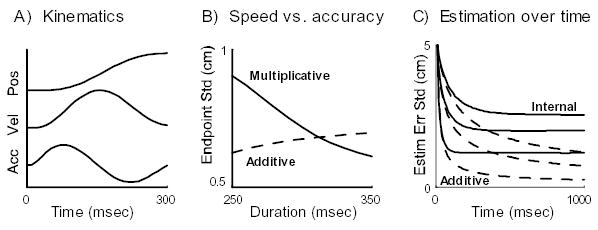
Figure 1.

A) Normalized position, velocity, and acceleration of the average trajectory of the optimal controller. B) A separate optimal controller was constructed for each instructed duration, the resulting closed-loop system was simulated for 10000 trials, and the positional standard deviation at the end of the trial was plotted. This was done with either Multiplicative (solid) or Additive (dashed) noise in the plant dynamics. C) The position of a stationary peripheral target was estimated over time, under Internal estimation noise (solid) or Additive observation noise (dashed). This was done in 3 sets of trials, with target positions sampled from Gaussians with means 5cm (bottom), 15cm (middle), and 25cm (top). Each curve is an average over 10000 simulation runs.

Another well-known property of reaching movements, first observed a century ago by Woodworth and later quantified as Fitts’law, is the trade-off between speed and accuracy. The fact that faster movements are less accurate implies that the instantaneous noise in the motor system is control-dependent, in agreement with direct measurements of isometric force fluctuations (Sutton and Sykes, 1967; Schmidt et al., 1979; Todorov, 2002) that show standard deviation increasing linearly with the mean. Naturally, this noise scaling has formed the basis of both closed-loop (Meyer et al., 1988; Hoff, 1992) and open-loop (Harris and Wolpert, 1998) optimization models of the speed-accuracy trade-off. Figure 1B illustrates the effect in our model: as the (specified) movement duration increases, the standard deviation of the endpoint error achieved by the optimal controller decreases. To emphasize the need for incorporating control-dependent noise, we modified the model by making the noise in the plant dynamics additive, with fixed magnitude chosen to match the average multiplicative noise magnitude over the range of movement durations. With that change, the endpoint error showed the opposite trend to the one observed experimentally (Figure 1B).

It is interesting to compare the effects of the control penalty r and the multiplicative noise scaling σ_c. As Eq 4 shows, both terms penalize large control signals –directly in the case of r, and indirectly (via increased uncertainty) in the case of σ_c. Consequently both terms lead to a negative bias in endpoint position (not shown), but the effect is much more pronounced for r. Another consequence of the fact that larger controls are more costly arises in the control of redundant systems, where the optimal strategy is to follow a “minimal intervention” principle, i.e. to leave task-irrelevant deviations from the average behavior uncorrected (Todorov and Jordan, 2002b; Todorov and Jordan, 2002a). Simulations have shown that this more complex effect is dependent on σ_c, and actually decreases when r is increased while σ_c is kept constant (Todorov and Jordan, 2002b).

Figure 1C shows simulation results from our second model, where the position of a stationary peripheral target is estimated by the optimal adaptive filter in Eq 8, operating under internal estimation noise or additive observation noise of the same magnitude. In each case, we show results for 3 sets of targets with varying average eccentricity. The standard deviations of the estimation error always reaches an asymptote (much faster in the case of internal noise). In the presence of internal noise this asymptote depends on target eccentricity; for the chosen model parameters the dependence is in quantitative agreement with our experimental results (Todorov, 1998). Under additive noise the error always asymptotes to 0.

7 Convergence properties

We studied the convergence properties of the algorithm in 10 models of psychophysical experiments taken from (Todorov and Jordan, 2002b), and 200 randomly generated models. The psychophysical models had dynamics and cost functions similar to the above example. They included two models of planar reaching, three models of passing through sequences of targets, one model of isometric force production, three models of tracking and reaching with a mechanically redundant arm, and one model of throwing. The dimensionalities of the state, control, and feedback were between 5 and 20, and the horizon n was about 100. The psychophysical models included control-dependent dynamics noise and additive observation noise, but no internal or state-dependent noise. The details of all these models are interesting from a Motor Control point of view, but we omit them here since they did not affect the convergence of the algorithm in any systematic way.

The random models were divided in two groups of 100 each –passively stable, with all eigenvalues of A being smaller than 1; and passively unstable, with the largest eigenvalue of A being between 1 and 2. The dynamics were restricted so that the last component of x_t was 1 –to make the random models more similar to the psychophysical models which always incorporated a constant in the state description. The state, control, and measurement dimensionalities were sampled uniformly between 5 and 20. The random models included all forms of noise allowed by Eq 1.

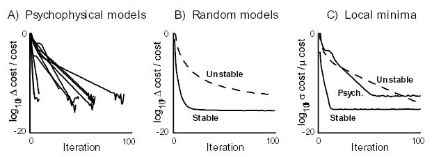
For each model, we initialized K_1…n−1 from Eq 2 and applied our iterative algorithm. In all cases convergence was very rapid (Figure 2A,B), with the relative change in expected cost decreasing exponentially. The jitter observed at the end of the minimization (Figure 2A) is due to numerical round-off errors (note the log scale), and continues indefinitely. The exponential convergence regime does not always start from the first iteration (Figure 2A). Similar behavior was observed for the absolute change in expected cost (not shown). As one would expect, random models with unstable passive dynamics converged more slowly than passively stable models. Convergence was observed in all cases.

Figure 2.

Relative change in expected cost as a function of iteration number, in A) psychophysical models, B) random models. C) Relative variability (std/mean) among expected costs obtained from 100 different runs of the algorithm on the same model (average over models in each class).

To test for the existence of local minima, we focused on 5 psychophysical models, 5 random stable, and 5 random unstable models. For each model the algorithm was initialized 100 times with different randomly chosen sequences K_1…n−1, and run for 100 iterations. For each model we computed the standard deviation of the expected cost obtained at each iteration, and divided by the mean expected cost at that iteration. The results, averaged within each model class, are plotted in Figure 2C. The negligibly small values after convergence indicate that the algorithm always finds the same solution. This was true for every model we studied, despite the fact that the random initialization sometimes produced very large initial costs. We also examined the K and L sequences found at the end of each run, and the differences seemed to be due to round-off errors. Thus we conjecture that the algorithm always converges to the globally optimal solution. So far we have not been able to prove this analytically, and cannot presently offer a satisfying intuitive explanation.

Note that the system can be unstable even for the optimal controller. Formally that does not affect the derivation, because in a discrete-time finite-horizon system all numbers remain finite. In practice the components of x_t can exceed the maximum floating point number whenever the eigenvalues of (A − BL_t) are sufficiently large. In the applications we are interested in (Todorov, 1998; Todorov and Jordan, 2002b) such problems were never encountered.

8 Improving performance via adaptive estimation

Although the iterative algorithm given by Eq 4 and Eq 7 is guaranteed to converge, and empirically it appears to converge to the globally optimal solution, performance can still be suboptimal due to the imposed restriction to non-adaptive filters. Here we present simulations aimed at quantifying this suboptimality.

Because the potential suboptimality arises from the restriction to non-adaptive filters, it is natural to ask what would happen if that restriction were removed in runtime, and the optimal adaptive linear filter from Eq 8 were used instead. Recall that although the control law is optimized under the assumption of a non-adaptive filter, it yields better performance if a different filter –that somehow achieves lower estimation error – is used in runtime. Thus in our first test we simply replace the non-adaptive filter with Eq 8 in runtime, and compute the reduction in expected total cost.

The above discussion suggests a possibility for further improvement. The control law is optimal with respect to some sequence of filter gains K_1…n−1. But the adaptive filter applied in runtime uses systematically different gains, because it achieves systematically lower estimation error. We can run our control law in conjunction with the adaptive filter, and find the average filter gains ${\tilde{K}}_{1\dots n-1}$ that are used online. Now, one would think that if we re-optimized the control law for the non-adaptive filter ${\tilde{K}}_{1\dots n-1}$ – which better reflects the gains being used online by the adaptive filter – this will further improve performance. This is the second test we apply.

As Figure 3 shows, neither method improves performance substantially for psychophysical models or random stable models. However, both methods result in substantial improvement for random unstable models. This is not surprising. In the passively stable models the differences between the expected and actual values of the states and controls are relatively small, and so the optimal nonadaptive filter is not that different from the optimal adaptive filter. The unstable models, on the other hand, are very sensitive to small perturbations and thus follow substantially different state-control trajectories in different simulation runs. So the advantage of adaptive filtering is much greater. Since musculoskeletal plants have stable passive dynamics, we conclude that our algorithm is well-suited for approximating the optimal sensorimotor system.

Figure 3.

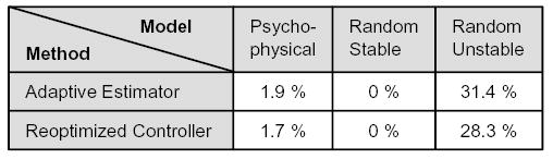
Numbers indicate percent improvement in expected total cost, relative to the cost of the solution found by our iterative algorithm. The two improvement methods are described in the text. Each method is applied to 10 models in each model class. For each model and method, expected total cost is computed from 10000 simulation runs. A value of 0% indicates that with a sample size of 10 models, the improvement was not significantly different from 0% (t-test, p=0.05 threshold).

It is interesting that control law re-optimization in addition to adaptive filtering is actually worse than adaptive filtering alone –contrary to our intuition. This was the case for every model we studied. Although it is not clear where the problem with the re-optimization method lies, this somewhat unexpected result provides further justification for the restriction we introduced. In particular, it suggests that the control law that is optimal under the best non-adaptive filter may be close to optimal under the best adaptive filter.

9 Discussion

Here we presented an algorithm for stochastic optimal control and estimation of partially-observable linear dynamical systems, subject to quadratic costs and noise processes characteristic of the sensorimotor system (Eq 1). We restricted our attention to controllers that use state estimates obtained by non-adaptive linear filters. The optimal control law for any such filter was shown to be linear, as given by Eq 4. The optimal non-adaptive linear filter for any linear control law is given by Eq 7. Iteration of Eq 4 and Eq 7 is guaranteed to converge to a filter and a control law optimal with respect to each other. We found numerically that convergence is exponential, local minima do not to exist, and the effects of assuming non-adaptive filtering are negligible for the control problems of interest. The application of the algorithm was illustrated in the context of reaching movements. The optimal adaptive filter (Eq 8), as well as the optimal controller for the fully-observable case (Eq 5), were also derived. To facilitate the application of our algorithm in the field of Motor Control and elsewhere, we have made a Matlab implementation available at www.cogsci.ucsd.edu/~todorov.

While our work was motivated by models of biological movement, the present results could be of interest to a wider audience. Problems with multiplicative noise have been studied in the optimal control literature, but most of that work has focused on the fully-observable case (Kleinman, 1969; McLane, 1971; Willems and Willems, 1976; Bensoussan, 1992; El Ghaoui, 1995; Beghi and D., 1998; Rami et al., 2001). Our Eq 5 is consistent with these results. The partially-observable case which we addressed (and which is most relevant to models of sensorimotor control) is much more complex, because the independence of estimation and control breaks down in the presence of signal-dependent noise. The work most similar to ours is (Pakshin, 1978) for discrete-time dynamics, and (Phillis, 1985) for continuous-time dynamics. These authors addressed a closely related problem using a different methodology. Instead of analyzing the closed-loop system directly, the filter and control gains were treated as open-loop controls to a modified deterministic dynamical system, whose cost function matches the expected cost of the original system. With that transformation it is possible to use Pontryagin’s Maximum Principle –which is only applicable to deterministic open-loop control –and obtain necessary conditions that the optimal filter and control gains must satisfy. Although our results were obtained independently, we have been able to verify that they are consistent with (Pakshin, 1978) by: removing from our model the internal estimation noise (which to our knowledge has not been studied before); combining Eq 4 and Eq 7; and applying certain algebraic transformations. However, our approach has three important advantages: (i) We managed to prove that the optimal control law is linear under a non-adaptive filter, while this linearity had to be assumed before. (ii) Using the optimal cost-to-go function to derive the optimal filter revealed that adaptive filtering improves performance, even though the control law is optimized for a non-adaptive filter. (iii) Most importantly, our approach yields a coordinate-descent algorithm with guaranteed convergence, as well as appealing numerical properties illustrated in Sections 7 and 8. Each of the two steps of our coordinate-descent algorithm is computed efficiently in a single pass through time. In contrast, application of Pontryagin’s Maximum Principle yields a system of coupled difference (Pakshin, 1978) or differential (Phillis, 1985) equations with boundary conditions at the initial and final time, but no algorithm for solving that system. In other words, earlier approaches obscure the key property we uncovered –which is that half of the problem can be solved efficiently given a solution to the other half.

Finally, there may be an efficient way to obtain a control law that achieves better performance under adaptive filtering. Our attempt to do so through re-optimization (Section 8) failed, but another approach is possible. Using the optimal adaptive filter (Eq 8) would make E [v_t+1] a complex function of ${\widehat{x}}_t,$u_t, and the resulting v_t would no longer be in the assumed parametric form (which is why we introduced the restriction to non-adaptive filters). But we could force that complex v_t in the desired form by approximating it with a quadratic in ${\widehat{x}}_t,$u_t. This yields additional terms in Eq 4. We have pursued this idea in our earlier work (Todorov, 1998); an independent but related method has been developed by (Moore et al., 1999). The problem with such approximations is that convergence guarantees no longer seem possible. While (Moore et al., 1999) did not illustrate their method with numerical examples, in our work we have found that the resulting algorithm is not always stable. These difficulties convinced us to abandon the earlier idea in favor of the methodology presented here. Nevertheless, approximations that take adaptive filtering into account may yield better control laws under certain conditions, and deserve further investigation. Note however that the resulting control laws will have to be used in conjunction with an adaptive filter –which is much less efficient in terms of online computation.

References

- Anderson F, Pandy M. Dynamic optimization of human walking. J Biomech Eng. 2001;123(5):381–390. doi: 10.1115/1.1392310. [DOI] [PubMed] [Google Scholar]
- Beghi ADd. Discrete-time optimal control with control-dependent noise and generalized Riccati difference equations. Automatica. 1998;34:1031–1034. [Google Scholar]
- Bensoussan, A. (1992). Stochastic Control of Partially Observable Systems Cambridge University Press, Cambridge.
- Bertsekas, D. and Tsitsiklis, J. (1997). Neuro-dynamic programming Athena Scientific, Belmont, MA.
- Burbeck C, Yap Y. Two mechanisms for localization? Evidence for separation-dependent and separation-independent processing of position information. Vision Research. 1990;30(5):739–750. doi: 10.1016/0042-6989(90)90099-7. [DOI] [PubMed] [Google Scholar]
- Chow C, Jacobson D. Studies of human locomotion via optimal programming. Math Biosciences. 1971;10:239–306. [Google Scholar]
- Davis, M. and Vinter, R. (1985). Stochastic Modelling and Control Chapman and Hall, London.
- El Ghaoui L. State-feedback control of systems of multiplicative noise via linear matrix inequalities. Systems and Control Letters. 1995;24:223–228. [Google Scholar]
- Flash T, Hogan N. The coordination of arm movements: an experimentally confirmed mathematical model. The Journal of Neuroscience. 1985;5(7):1688–1703. doi: 10.1523/JNEUROSCI.05-07-01688.1985. [DOI] [PMC free article] [PubMed] [Google Scholar]
- Harris C, Wolpert D. Signal-dependent noise determines motor planning. Nature. 1998;394:780–784. doi: 10.1038/29528. [DOI] [PubMed] [Google Scholar]
- Hatze H, Buys J. Energy-optimal controls in the mammalian neuromuscular system. Biol Cybern. 1977;27(1):9–20. doi: 10.1007/BF00357705. [DOI] [PubMed] [Google Scholar]
- Hoff, B. (1992). A computational description of the organization of human reaching and prehension Ph.D. Thesis, University of Southern California.
- Jacobson, D. and Mayne, D. (1970). Differential Dynamic Programming Elsevier, New York.
- Jones K, Hamilton A, Wolpert D. Sources of signal-dependent noise during isometric force production. Journal of Neurophysiology. 2002;88:1533–1544. doi: 10.1152/jn.2002.88.3.1533. [DOI] [PubMed] [Google Scholar]
- Kleinman D. Optimal stationary control of linear systems with control-dependent noise. IEEE Transactions on Automatic Control. 1969;AC-14(6):673–677. [Google Scholar]
- Kording K, Wolpert D. The loss function of sensorimotor learning. Proceedings of the National Academy of Sciences. 2004;101:9839–9842. doi: 10.1073/pnas.0308394101. [DOI] [PMC free article] [PubMed] [Google Scholar]
- Kuo A. An optimal control model for analyzing human postural balance. IEEE Transactions on Biomedical Engineering. 1995;42:87–101. doi: 10.1109/10.362914. [DOI] [PubMed] [Google Scholar]
- Kushner, H. and Dupuis, P. (2001). Numerical Methods for Stochastic Optimal Control Porblems in Continuous Time Springer, New York, 2 edition.
- Li, W. and Todorov, E. (2004). Iterative linear-quadratic regulator design for nonlinear biological movement systems. In 1st International Conference on Informatics in Control, Automation and Robotics
- Loeb G, Levine W, He J. Understanding sensorimotor feedback through optimal control. Cold Spring Harb Symp Quant Biol. 1990;55:791–803. doi: 10.1101/sqb.1990.055.01.074. [DOI] [PubMed] [Google Scholar]
- McLane P. Optimal stochastic control of linear systems with state- and control-dependent disturbances. IEEE Transactions on Automatic Control. 1971;AC-16(6):793–798. [Google Scholar]
- Meyer D, Abrams R, Kornblum S, Wright C, Smith J. Optimality in human motor performance: Ideal control of rapid aimed movements. Psychological Review. 1988;95:340–370. doi: 10.1037/0033-295x.95.3.340. [DOI] [PubMed] [Google Scholar]
- Moore J, Zhou X, Lim A. Discrete time LQG controls with control dependent noise. Systems and Control Letters. 1999;36:199–206. [Google Scholar]
- Nelson W. Physical principles for economies of skilled movements. Biological Cybernetics. 1983;46:135–147. doi: 10.1007/BF00339982. [DOI] [PubMed] [Google Scholar]
- Pakshin P. State estimation and control synthesis for discrete linear systems with additive and multiplicative noise. Avtomatika i Telemetrika. 1978;4:75–85. [Google Scholar]
- Phillis Y. Controller design of systems with multiplicative noise. IEEE Transactions on Automatic Control. 1985;AC-30(10):1017–1019. [Google Scholar]
- Rami M, Chen X, Moore J. Solvability and asymptotic behavior of generalized Riccati equations arising in indefinite stochastic LQ problems. IEEE Transactions on Automatic Control. 2001;46(3):428–440. [Google Scholar]
- Schmidt R, Zelaznik H, Hawkins B, Frank J, Quinn J. Motor-output variability: a theory for the accuracy of rapid notor acts. Psychol Rev. 1979;86(5):415–451. [PubMed] [Google Scholar]
- Sutton G, Sykes K. The variation of hand tremor with force in healthy subjects. Journal of Physiology. 1967;191(3):699–711. doi: 10.1113/jphysiol.1967.sp008276. [DOI] [PMC free article] [PubMed] [Google Scholar]
- Sutton, R. and Barto, A. (1998). Reinforcement Learning: An Introduction MIT Press, Cambridge MA.
- Todorov, E. (1998). Studies of goal-directed movements Ph.D. Thesis, Massachusetts Institute of Technology.
- Todorov E. Cosine tuning minimizes motor errors. Neural Computation. 2002;14(6):1233–1260. doi: 10.1162/089976602753712918. [DOI] [PubMed] [Google Scholar]
- Todorov E. Optimality principles in sensorimotor control. Nature Neuroscience. 2004;7(9):907–915. doi: 10.1038/nn1309. [DOI] [PMC free article] [PubMed] [Google Scholar]
- Todorov, E. and Jordan, M. (2002a). A minimal intervention principle for coordinated movement. In Becker, S., Thrun, S., and Obermayer, K., editors, Advances in Neural Information Processing Systems 15, pages 27–34. MIT Press, Cambridge, MA.
- Todorov E, Jordan M. Optimal feedback control as a theory of motor coordination. Nature Neuroscience. 2002b;5(11):1226–1235. doi: 10.1038/nn963. [DOI] [PubMed] [Google Scholar]
- Todorov, E. and Li, W. (2004). A generalized iterative LQG method for locally-optimal feedback control of constrained nonlinear stochastic systems. Submitted to the American Control Conference
- Uno Y, Kawato M, Suzuki R. Formation and control of optimal trajectory in human multijoint arm movement: Minimum torque-change model. Biological Cybernetics. 1989;61:89–101. doi: 10.1007/BF00204593. [DOI] [PubMed] [Google Scholar]
- Whitaker D, Latham K. Disentangling the role of spatial scale, separation and eccentricity in weber’s law for position. Vision Research. 1997;37(5):515–524. doi: 10.1016/s0042-6989(96)00202-7. [DOI] [PubMed] [Google Scholar]
- Whittle, P. (1990). Risk-Sensitive Optimal Control John Wiley and Sons, New York.
- Willems JL, Willems JC. Feedback stabilizability for stochastic systems with state and control dependent noise. Automatica. 1976;1976:277–283. [Google Scholar]
- Winter, D. (1990). Biomechanics and Motor Control of Human Movement John Wiley and Sons, New York.