The Evolution of DNA Regulatory Regions for Proteo-Gamma Bacteria by Interspecies Comparisons

Abstract

The comparison of homologous noncoding DNA for organisms a suitable evolutionary distance apart is a powerful tool for the identification of cis regulatory elements for transcription and translation and for the study of how they assemble into functional modules. We have fit the three parameters of an affine global probabilistic alignment algorithm to establish the background mutation rate of noncoding seqeunce between E. coli and a series of gamma proteobacteria ranging from Salmonella to Vibrio. The lower bound we find to the neutral mutation rate is sufficiently high, even for Salmonella, that most of the conservation of noncoding sequence is indicative of selective pressures rather than of insufficient time to evolve. We then use a local version of the alignment algorithm combined with our inferred background mutation rate to assign a significance to the degree of local sequence conservation between orthologous genes, and thereby deduce a probability profile for the upstream regulatory region of all E. coli protein-coding genes. We recover 75%–85% (depending on significance level) of all regulatory sites from a standard compilation for E. coli, and 66%–85% of sigma sites.

We also trace the evolution of known regulatory sites and the groups associated with a given transcription factor. Furthermore, we find that approximately one-third of paralogous gene pairs in E. coli have a significant degree of correlation in their regulatory sequence. Finally, we demonstrate an inverse correlation between the rate of evolution of transcription factors and the number of genes they regulate. Our predictions are available at http://www.physics.rockefeller.edu/^∼siggia.[Online supplemental material available at http://www.genome.org.]

Functional genomics has made great progress in the prediction of protein coding regions using Markov models whose hidden states encode the components of a gene (promoter, exon, intron, splice sites) and whose parameters are fit to known instances of these states. Annotating the regions of the genome that control transcription and translation has proved more refractory. The binding site for a single protein is much smaller than a typical exon and regulatory proteins work in modules, but we know nothing about the syntax governing the assembly of functional modules, there is no counterpart to cDNA libraries to tell us which bits of sequence belong to a common module, and there is no analogue to the extensive libraries of known proteins to compare against.

Regulatory sequences occur in multiple copies in a single genome, which is the basis for their detection computationally. Strategies range from the prediction of a single weight matrix motif for a cluster of genes (Stormo and Hartzell 1989; Lawrence et al. 1993; Bailey and Elkan 1994) to string counts with probabilities assigned with reference to genes not in the cluster (van Helden et al. 1998; Brazma et al. 1998), and finally fits to more elaborate models for all regulatory regions in the genome and the simultaneous determination of many putative motifs at once (Bussemaker et al. 2000). DNA microarray experiments have been a boon to studies of gene regulation because they provide complete sets of covarying genes. However, they also quantify how much more remains to be understood. In yeast, most copies (e.g., 75%) of the canonical control elements for cell cycle and sporulation occur in the upstream regions of nonresponding genes (Bussemaker et al. 2001). Hence there are other sequence signals to be found, but probabilistic methods on a single genome encounter the fundamental problem that there is never a single sharp secondary motif that delimits the active from inactive class, but many marginally significant ones.

The availability of genomic sequence for related species compensates for the greater plasticity of regulatory sequence modules (compared to proteins) and makes interspecies comparison a powerful technique for their identification. There have been studies of the globin locus across many species (Stojonovic et al. 1998), comparisons of several Drosophila species (Blanchette et al. 2000), and many mouse comparisons (Hardison et al. 1997; Loots et al. 2000; Wasserman et al. 2000). For prokaryotes, a broad collection of fully sequenced genomes was examined by McGuire et al. (2000), and more limited comparisons were made by Gelfand et al. (2000). A recent study by McCue et al. (2001) uses many of the same organisms we do, but a complementary algorithm. Comparisons with prior work are reserved for the Discussion herein.

In this paper we address the intertwined questions of how rapidly do gene control regions evolve and what are the most informative species pairs to study for the elucidation of cis regulatory regions. We work primarily at the module or locus level and only as a second step discern individual protein binding sites. We thus impose no preconceptions about what aspects of the module are most important (as measured by conservation) to the regulatory net of the cell. Escherichia coli is the most useful species to examine at the moment since it is the best studied prokaryote and has the densest set of related genomes in various stages of sequencing. Although in the future, sequencing projects may be undertaken largely to ascertain regulatory sites, the regulatory system of E. coli is not simple; there are seven sigma factors and several other regulatory proteins (e.g., crp and lrp) that control many operons, plus several factors with widespread activity that facilitate contacts between other factors (e.g., fis, ihf, hns) (Lin and Lynch 1995). There are also cis elements regulating translation which are much more extensive that the core Shine Dalgarno sequence (Lin and Lynch 1995). All are fused together in the several hundred bases upstream from translation start (Gralla and Collado-Vides 1996). In public databases are approximately 800 protein binding sites (including sigma sites) regulating ∼400 genes or about 10% of all operons (Robison et al. 1998; Salgado et al. 2000b).

Our alignment algorithm, which is essential to comprehension of our results, is described in the Methods section.

METHODS

Alignment Algorithm

Sequence alignments (e.g., BLAST) are generally done with predetermined penalties for mutations and gaps, and assign a probability to the best score thus obtained based on a null model of completely uncorrelated sequence pairs. This naturally responds to the question of whether the query sequence, run against the database, has a better score than chance alone would suggest. Frequently a scoring scheme adapted to the evolutionary distance of the match one is exploring will enhance the significance of the relevant matches compared to others, but in all cases significance is assessed relative to the probability that two random sequences (with the residue frequencies of the database) would score as well as the putative functional match.

Our task is more difficult. Since we are comparing organisms which are manifestly related, we first have to fit an evolutionary model to determine as best possible the neutral or basal evolution rate (Thorne et al. 1991). With respect to this correlated model, we must then ascertain whether certain regions of sequence are more similar than expected, and thereby score them as functional. In practice, it is impossible to know what if any regions of the genome are not subject to fitness constraints, and for bacteria, lateral gene transfer is so common that one may question whether the most recent common ancestor is a well defined concept. (Since we examine relatively close organisms and look at the entire genome, lateral gene transfer should not contaminate most of our results.) Thus, operationally we compute the basal evolution rate as the most rapid evolution we can find for a substantial block of manifestly homologous sequence, pooled from multiple regions of the genome. Further details are given in the Results section.

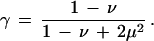
We rather conventionally describe sequence evolution in terms of three processes, a single base mutation, a gap opening, and a gap extension. More precisely,

1

2

where λ sets the rate of base substitutions (b → b′), and μ, ν are the gap opening and extension parameters. We use these parameters within a probabilistic alignment algorithm based on that of Yu and Hwa (2001) (with our modifications detailed in the Appendix). Probabilistic alignment computes the sum of all ways of turning sequence 1 into sequence 2, with each weighted by the number of mutations and insertion-deletions required. (In its global form, it requires boundary conditions which reflect whether there are conserved landmarks, that is, unique homologous genes, on one or both ends of the intergenic regions being fit.) The resulting score can be interpreted as a probability distribution over all pairs of sequences, since it is positive and sums to one (see Appendix). Probabilistic alignment is particularly natural in our context, since the same (global) algorithm can be used both to fit parameters and score pairs of sequences and admits an interpretation in terms of an explicit generation process. That is, if we fit our three parameters to a pair of sequences by maximum likelihood (i.e., maximizing the score given the data), then there exists a Markov model (Yu and Hwa 2001) which uses these parameters and generates from one sequence via insertions, deletions, and mutations a second sequence such that when parameters are fit to this new synthetic sequence pair, the generating values are recovered. The local alignment of Yu and Hwa (2001) assigns probabilities to all possible ways of drawing subregions from the two sequences. When looking at many sequence pairs together, it is important not to report just the best local alignment for a given pair, because ultimately we must make a decision about E. coli based on all the comparison species.

Our local version of probabilistic alignment is complicated by the fact that we want to assign significance relative to a neutral model described by the three parameters above. Since we are looking for protein binding sites, we assume zero gap parameters and a new substitution parameter κ subject to κ < λ which we adjust to optimize significance. (Our scoring formula is given by Eq. A.6.) With κ = 0, we would score positively only regions with no mutations but then assign them higher significance than for any κ > 0. If κ approaches the background level, then all regions would be assigned marginal significance. Thus for each homologous upstream region in each pair of organisms, we scanned over κ to maximize the significance of the highest scoring region. On average, κ was smaller when comparing E. coli with Salmonella than E. coli with Vibrio, but there was considerable variability among genes.

The local alignment then yields diagonal segments of high significance in the rectangle defined by running the two sequences along the x and y axes. To obtain a conventional graph, we take the maximum significance calculated for each E. coli base ( and any base of the comparison species) and plot it as a function of upstream position in E. coli. Note that the blocks of high significance in this graph need not occur in the same order in the other species as in E. coli, and it should be checked that the blocks indeed correspond to contiguous bases in the other sequence.

Statistical Tests

Based on the size of the typical upstream region (300–500 bp) that we scan over with our local algorithm, a marginally significant log odds score in our units is ∼6, i.e., ln(500). A single score can be deduced from a collection of pairwise alignments by either of two methods which make opposite assumptions about the sequences being compared with E. coli; the truth is somewhere in between. Either take an envelope of all log odds profiles (if the comparison sequences are maximally correlated) or take a sum if they are completely uncorrelated. In the latter case, to filter noise we only consider those bases in each pairwise comparison where the log odds score is over 9, otherwise it is omitted from the sum.

In order to extract a series of disjoint high significance intervals from the log odds graph to compare with footprinted factor binding sites, we used an edge detection heuristic defined by computing the derivative with respect to position and thresholding. What fell between successive bands of positive and negative derivatives subject to some plausible length limitations was the prediction.

For measuring the similarity between a set of predicted sequence intervals and the experimental data base, we define a hit (following McCue et al. 2001) as any overlap. A single prediction can hit multiple sites if they are nearby or nested, and the score h_s for a given E. coli control region is just the total number of hits. The score expected by chance is computed by fixing the predictions and randomizing the positions of the experimental sites individually, subject only to the constraint that the distribution of positions for each site matches that for all sites in the database. The average 〈h〉 and variance 〈(h − 〈h〉)²〉 in the number of hits are computed separately for each site, and summed over all sites in the regulatory region to give 〈h_s〉 and ν_s = 〈(h_s − 〈h_s〉)²〉, respectively. The significance is then parameterized by

3

This quantity is not Gaussianly distributed and does not readily translate into a probability, but serves as a quality measure for the predictions for each upstream segment.

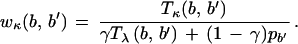
Given a set of N aligned sequences with n copies of base b in position i, we define a (frequency) weight matrix w and a score s for a sequence (b₁, b₂, . . ) as did Robison et al. (1998),

4

where p_b is the background probability for upstream regions (0.3 for A, T). The average of s for all N aligned sequences relative to the average for background sequence is a measure of the specificity of the weight matrix.

Extracting Homologous Regions From Genomic Data

The key to our method is the selection of pairs of organisms which give the most informative comparisons. Figure 1 gives the rRNA phylogeny of the species we have examined. We do not require a fully assembled sequence, merely large enough contigs to give a good protein match plus ∼500 bp upstream of AUG, which is where almost all control elements are found (Gralla and Collado-Vides 1996).

Figure 1.

Phylogeny of relevant bacterial species. The three-letter abbreviations are as follows: eco, Escherichia coli K12 (genbank entry NC_000913); stm, Salmonella typhimurium LT2 (genome.wustl.edu/gsc/bacterial/salmonella.shtml); kpn, Klebsiella pneumoniae MGH78578 (genome.wustl.edu/gsc/Projects/bacterial/klebsiella.shtml); ype, Yersinia pestis CO-92 (www.sanger.ac.uk/Projects/Y_pestis/); vcb, Vibrio cholerae N16961 (genbank NC_002505 and NC_002506); hin, Haemophilus influenzae Rd (genbank NC_000907). The phylogenetic tree is based on 16S ribosomal RNA sequences. H. influenzae is shown only for comparative purposes and was not analyzed in our study.

We used the program tfastx (Pearson 1999) and a spectrum of scoring matrices to match each of the ∼4200 orfs in E. coli (represented as a protein sequence) against all other genomic sequences including E. coli itself (to detect paralogous genes). Since we are examining very similar species we can insist on a stringent match criterion of a probability score <10⁻²⁵ (10⁻⁵ would be marginal in these units), and at least 40% identity as defined by the program. We assembled all valid hits into disjoint closed intervals on the target genome, which frequently began with the first amino acid of the query protein. When a given protein had several distinct hits, we ordered them by probability score, and then by percent identity (probability scores often underflowed to 0). We restricted attention to upstream control regions that did not overlap any annotated coding region on either strand, were at least 50 bp in length and were cutoff at 500 bp. The minimum length restricts us to approximately one promoter per operon (Salgado et al. 2000a). Table 1 gives the statistics of our matches, and Table 2 a breakdown of the number of conserved gene pairs between organisms. The subclass of noncoding regions between two conserved pairs will be useful in what follows.

Table 1.

Statistics for the Matches of the 4241 E. coli Genes used as Queries Against the Target Genomes Given in the Column Heading

Number of:	eco	stm	kpn	ype	vch
All matches	5987	4429	4497	3103	2285
orfs with ≥1 match	4241	3250	3047	2425	1695
Unique matches	3414	2567	2301	2013	1385
Orth. upstream regions	2574	1928	1752	1424	936

The first row counts all distinct matches in the target; the second row gives the number of queries with a valid match; the third row counts how many of the 4241 queries had a unique match within our threshold (score <10⁻²⁵ and percent identity over 40%); and the last row are all those unique matches that have at least 50 bases upstream that do not overlap coding sequence on either strand. There are 2127 E. coli genes that have orthologous upstream region in at least one organism, and 768 genes with an orthologue in all four species. 

Table 2.

Statistics for the Preservation of Three Categories of Contiguous Pairs of E. coli Genes Separated by between 1 and 500 Non-Coding Bases

Number of gene pairs:	eco	stm	kpn	ype	vch
tandem (same strand)	2388	1045	729	547	252
divergently transcribed	552	305	204	123	34
convergently transcribed	517	222	53	36	7

The genes matched are further restricted to those in the third row of Table 1, with a unique match which begins within the first (last) six residues of the query gene (with first/last chosen so that the inter gene region is well delineated). 

As a database of known E. coli protein binding sites, we used the compilation of Robison et al. (1998) and a related set from McCue et al. (2001).

RESULTS

Prediction of Functional Regulatory Sites

For the compact genomes of prokaryotes, it is by no means obvious what regions of the genome are not subject to selective pressure and thus suitable for estimating a mutation rate against which to measure the degree of conservation of the promoters. The most propitious regions to examine are those between conserved gene pairs, because the intervening sequence should all be homologous under our assumptions and we can use fixed boundary conditions on both ends to do the global alignment. In Table 2 we show that the ratio of divergent gene pairs (common upstream region, e.g., 5′ 5′ pairs) to convergent ones (sharing a noncoding terminal region, e.g., 3′3′ pairs), increases significantly as one moves from Salmonella to Vibrio. This finding confirms, without any potential biases as to where experiments looked, the general observation that most cis regulatory elements in bacteria are upstream of the gene, not downstream. We examined the set of convergently transcribed (i.e., 3′ 3′) gene pairs; a small number of these were dropped which had significant amounts of conservation either because of recent lateral gene transfer, or some functional secondary structure that still retains some primary sequence homology. This is legitimate because we are looking for nonfunctional, neutrally evolving sequence. The homology of the regions being compared is guaranteed by the good match between the bracketing gene pairs. From the remaining set, upwards of a kilobase of sequence from several such pairs was fit with a single set of parameters. These fits were stable for other selections of sequence.

As seen in Table 3 part b, only Salmonella retains some degree of correlation in minimally functional regions; the other pairs of species are random (i.e., the optimal fit corresponds to a point mutation rate of chance). These fits are conservative, since they are a lower bound to the neutral mutation rate and thus the statistical significance of any feature we find in the E. coli control region will be higher than we report, given our model. For comparison, the same fits were done for gene pairs with a common 5′ control region and show much higher conservation.

Table 3.

Fits of the Evolutionary Parameters to a Subset of the Conserved Gene Pairs from Table 2 for the Categories Indicated

Table 3A. Tandem conserved gene pairs
	stm	kpn	ype	vch
μ	0.02	0.03	0.05	0.19
ν	0.96	0.92	0.93	0.68
λ	0.05	0.06	0.08	0.14

Table 3B. Convergently transcribed, conserved pairs
	stm	kpn	ype	vch
μ	0.09	0.02	0	0
ν	0.9	0.9	0	0
λ	0.16	0.24	0.25	0.25

Error bars for μ, ν, and λ are within 10%, respectively. The pairs were subject to the additional constraints that the intergenic region was between 70 and 500 bp in length; and for the convergent pairs, without obvious conserved blocks (i.e., max score <12). At least a kb of sequence was fit in all cases. 

Our evolution model fits were then used to assign a significance to matches between ungapped regions for all orthologous upstream regions. Examples are given in Figures 2 and 3. As noted in the Methods section, the κ parameter can be adjusted to optimize significance. A small κ gives sharp delineation but poor overall structure since it only selects perfectly conserved blocks. The significance generally rises as κ increase from ∼0 and then declines unless the entire upstream region merges into one block and our probability calculation ceases to be valid. For the more distant species, ype and vch, a suitable automatic way of adjusting κ is to maximize the root mean square fluctuation in the log probability profile. For stm and kpn however, we imposed in addition an upper bound of 0.004 and 0.006 respectively on κ, which aids in the delineation of sites.

Figure 2.

The probability profiles for the orthologous region upstream of the gene lpdA (lipoamide dehydrognease (NADH). The abscissa is in bp units, and the start codon for lpdA begins at position 325. In (a), κ = 0 for all species, whereas in (b) it is optimized separately in each case (as explained in the text), which yields κ = 0.006, 0.003, 0.01, and 0.06 for kpn, stm, vch, and ype, respectively. The two known factor binding sites for sigma 70 (rpoD17) and an anaerobic factor arcA are marked. In (b), the predictions of McCue et al. (2001) are marked with “W” and the remaining bars are our predictions from the summed profiles.

Figure 3.

The probability profiles for the intergenic region between the conserved divergently transcribed pair of E. coli genes, yfhD to the left and purL to the right, whose 5′ end begins at position = 396. An optimal κ = 0.006, 0.001, 0, 0.003 was determined for kpn, stm, vch, and ype, respectively. There is only one documented binding site for purine repressor (purR). The predictions of McCue et al. (2001) for both genes are combined without distinction and labeled with “W”.

In Figure 2, we contrast κ = 0 with what we consider the optimal κ for each organism. Notice that the sum delineates the overlapping annotated sites better than does the envelope. The maximum for all four organisms falls on top of the annotated sites in Figure 2b, whereas with κ = 0 the maximum for ype is around i = 25. The second most prominent structure in Figure 2 does not get any contribution from stm, and broadens when κ is fit. The third structure around i = 300 only rises above the cutoff of 9 in Figure 2b. The genome-wide statistics of the intervals we flag as significant, such as those shown in Figure 2b, are discussed below.

Figure 3 shows the intergenic region between a pair of divergently transcribed genes which were conserved for all four species. There is only one documented site and it appears as a ‘hat’ on top of the largest block which reflects its presence in vch, which is contributing nothing elsewhere to the summed profile. In the next most significant block around 125, ype doe not follow kpn and stm as is true elsewhere. Perhaps the offset lobe of signal for ype is moderating the left gene rather than the right one.

Our complete set of predictions are available on the Web. It remains true genome-wide that when properly discounted by evolutionary distance, Salmonella (an organism so close to E. coli that recombination between the genomes is possible; Rayssiguier et al. 1989) is both informative yet does not dominate the comparisons.

Though it is not our primary purpose to predict individual transcription factor binding sites, it is obviously important to show that the known sites fall within our conserved regions and to put a significance value on our predictions (e.g., if we claim that most of the upstream region is conserved, as sometimes occurs when it is short, our significance is low). To compare with McCue et al. (2001), who used a multiple alignment tool which assumes a null model of mutually uncorrelated data segments, we took the sum of all our pairwise alignments over a significance threshold of 9 (cf. Figs. 2, 3) position by position along the E. coli reference sequence. We then made two categories of predictions, both genome-wide: a single best prediction for each gene, and all significant segments. Two data sets of known regulatory sites were used, those upstream of the 184 ‘test set’ genes of McCue et al. (2001), Table 4 (with and without the sigma sites from Robison et al. 1998), and simply all sites from Robison et al. (1998), Table 5. Any comparisons with the results of McCue et al. (2001) are approximate because we focused on different aspects of the signal; for example, they excluded sigma sites by fitting to a palindromic model, whereas we do not distinguish them. Further comparison is deferred until the Discussion. Gene by gene the statistical significance is low, because as is evident from Figures 2 and 3, a good portion of the upstream region seems functional; we predict 3141 sites (with an average length of 32 bases) for 2127 upstream regions. In addition, our estimate for the number of sites hit by chance was high, because we randomized each experimental site independently even if several of them overlapped.

Table 4.

The Percentage of Times our Single Best Prediction per Gene Hits a Known Site in the McCue et al. (2001) Study Set with and without Sigma Sites

	Without σ sites	With σ sites
This study	72.8%	75.5%
McCue et al. 2001	79.8%	82.0%

Our prediction consists of the 24 highest scoring sites around the maximum, as explained in the text. In a significant number of cases the corresponding best prediction from McCue et al. (2001) consists of several sites with a degenerate score. We made no prediction for 37 of the 183 genes in the study set, either because we had no homologue or no score above threshold. Our percentages are calculated with respect to the 146 genes where a prediction was made. 

Table 5.

Match of All Significant Predictions to the Data of Robison et al. (1998)

	Hit score	z-score >1	z-score >2
This study	85.7%	27.5%	6.7%
McCue et al. 2001	86.1%	26.5%	5.2%

The percentages are calculated with respect to the number of genes with a positive prediction: 349 for the first row and 388 for the second. The columns denote the fraction of sites hit and the percentage of genes for which the number of experimental sites hit has a statistical significance (defined by the z-score in equation 3) greater than 1, 2. 

Analysis of the Upstream Regions of Paralogous Pairs

Our interspecies comparisons can be trivially extended to paralogous pairs of genes within E. coli. There are 169 unique gene pairs which satisfy the stringent cutoffs defined for the last line of Table 1. We ran our local alignment procedure on each pair and assumed a completely random background evolution model. The parameter κ was optimized with an upper cutoff of 0.1. The maximum log odds score exceeded 9 for 52 of these pairs which are listed on our website along with their GENBANK annotation, and alignments. Of the 52, ten are transposon-related ORFs (using Riley's functional classification 5.1.4; see http://genprotec.mbl.edu:80/start) and are grouped separately since their upstream conserved regions are presumably not conventional transcription factor binding sites. There was no correlation between the maximum score for the upstream region and the percent identity between the paralogous proteins.

Correlation between Gene Function and Conservation of Upstream Region

We have investigated how a quantitative measure of the conservation of orthologous upstream regions, the maximum log odds score, correlates with the functional class of the respective genes. We restricted the maximum to a region of 300 nucleotides upstream of the translation start of the gene in order to avoid spurious signal from divergently transcribed genes. It is already interesting to simply rank all 2127 genes for which we have orthologs by this score (details on our web site). Perhaps not very surprisingly, all the ribosomal genes get very high scores; all 20 are ranked above 365, and five (rpmB, rplJ, rpsT, rpsF, rplM) are among the top 30 genes. Interestingly, there are seven genes (ORFS) with no known function (Riley category 0.0.0 and “hypothetical protein”) among the top 30 (yhbC, yafB, ybeB, yeaA, yaeO, yeaQ, yhdG).

Restricting attention to the 768 genes with orthologues in all four species, we made a histogram of the maximum log odds score (summed over the four species) for the 239 genes with no known function and compared with the corresponding histogram for the functionally annotated genes (Fig. 4). The latter group gave better scores, and the probability that the histograms came from a common distribution was less than 0.07 as defined by a χ² test. We examined other functional groupings from Riley's classification (e.g., metabolism or DNA replication/repair) but could find no other correlations as strong as that for the ribosomal genes.

Figure 4.

Normalized score histograms of genes with known function and genes with unknown function.

Evolution of Known Regulatory Sites

For each site annotated to control a particular gene in E. coli, we mapped it into the upstream region of homologous genes by two methods with different biases. The first scheme simply looked for the minimal number of mutations and in the one orientation of site relative to gene defined by E. coli. We accepted a match in the target species only when the probability of a chance match was small, and the match was unique (e.g., when there are two copies of the same site upstream, each must have a unique match). Under this mapping, the number of sites identified in the target species decreased with increasing evolutionary distance, and the weight matrix computed from all the mapped sites for a given factor was less specific than that in E. coli. (Comparing with ype, the average score of the defining sites against the weight matrix, decreased by 2× for crp and rpoD (sigma 70), was unchanged for lexA, and other factors fell in between.)

An alternative mapping of sites assumes that the regulatory network is preserved, that is, homologous genes must be regulated by the same factors though copy number can change. Therefore, the factor's weight matrix in E. coli was used to find the best match in the homologous upstream region. Thus virtually all sites are matched, and we find the specificity of the weight matrix defined by the mapped sites to be generally the same as in E. coli. This mapping of course contains a bias towards good sites in the target species, and to control for this we randomized the upstream regions and remapped. Now the specificity of the weight matrix defined by the mapped sites decreases by 1/2–1/3, except for less specific factors such as cytR, fis, flhCD, gcvA, hipB, his, lrp, rhoD, and rpoS. On this basis, we can say that the regulatory network is approximately preserved between the organisms we examine. Mapping by weight matrix is similar to what the transcription factor ‘sees’ (assuming the DNA binding domain has not changed) if we can take the weight matrix score as a surrogate for the binding energy.

Under either mapping, the ratio of transversions to transitions was around 1:1 when comparing E. coli and Salmonella and 2:1 for most factors in more distant pairs of species. The 2:1 ratio is expected when all base changes are equally likely. For factors with many known sites, we have adequate statistics to show that the number of mutations per site negatively correlates with the information score or specificity of the site. By this measure, the pattern of change between species is similar to that intraspecies.

In the aggregate, we expect that homologous genes are regulated in comparable ways within the species we are examining. Thus most mutations between homologous upstream regions should be neutral. To project this information onto a plausible subspace to analyze quantitatively, we asked whether mutations in a factor binding site tend to compensate so as to preserve the weight matrix score (again taken as a surrogate for the binding energy). We scored each site against the weight matrix for the respective species, ignored the least significant bases, and considered only pairs of homologous sites for which there were two or more mutations (so that compensation is a possibility). Let P be the set of bases within the site (numbered from left to right) which change, and m the score from the base at position i in the weight matrix, Eq. (4). Then for each pair of homologous sites define x = (∑_Pm − m)²/∑_P(m − m)². We defined x so that if the individual differences for each i in the numerator were random, then the average of x (approximated by summing over all valid pairs of sites for a given factor) would be one. Thus an average less than one indicates correlated changes. Within the scatter, which was substantial, we found no evidence for correlated changes in weight matrix score. The exceptional cases (e.g., for rpoD17, only 8 out of 95 pairs of sites had x > 1) could be attributed to biases in the selection of sites with a weight matrix that was itself not very specific. When we mapped the sites for this factor by minimizing the total number of mutations, x-average was >1. Of course this mapping attributes as much weight to the nonconserved positions as the functional ones, so biases in the other direction.

For the sigma factors, it is known that sites downstream of the binding site can significantly affect the rate of transcription (McClure et al. 1983). We found however that the mutation rate in the 16 sites downstream of the rpoD17 binding site was nearly as high as in the middle (i.e., the nonconserved region) of the binding site itself. Similarly, no meaningful reduction in the transition or transversion rates upstream of the binding site was observed (Estrem et al. 1998).

Evolution of Transcription Factors

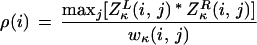
Clearly the evolution of binding sites is correlated with the proteins that bind there, so in cases where an E. coli factor-DNA cocrystal was available (Table 6), we analyzed the conservation of the set of residues R defined in the structure paper to be in contact with the DNA. For each species, the protein sequence for the E. coli factor was aligned to the orthologous protein using tfastx (see the Methods section). Since our proteins are very well conserved and there were virtually no gaps in the regions of interest, more elaborate protein family alignments were not necessary. Even for vch, in half of the factors all residues in R are conserved. In fact for Crp, 96% of all residues are conserved between E. coli and Vibrio (vs. an average of 0.66 ± 0.15 for these species). However contrary to our expectation, the number of mutations found among the residues from R was consistent with the percent identity (PID) computed for the entire protein alignment. This observation allows us to use all the known factors and ask whether the evolution rate of the factor as defined by its PID relative to one, 1-PID, correlates with the number of sites that it regulates. The number of regulated sites we approximate (Robison et al. 1998) by the weight matrix score of the experimental sites relative to background normalized by the combined variance, σ, viz,

5

The expectation that large regulons evolve more slowly than small ones is indeed born out in Figure 5 for vch. (The same correlation is observed for other species but the slope is less.)

Table 6.

Conservation of Residues that Affect DNA Binding Specificity across Orthologues

	stm	kpn	ype	vch
AraC	+	+	−	−
Crp	+	+	+	+
MetJ	+	+	+	+
OmpR	+	+	+	−
RpoD	+	+	+	+
SoxS	?	−	−	−
TrpR	+	?	?	−

Each row lists data for an E. coli transcription factor where the crystal structure and information about residues that are important for DNA binding specificity are available. We list the literature reference and our evaluation of the conservedness of these residues for each species. A plus (minus) sign denotes conserved (not conserved), a question mark stands for unclear cases (for example, a frame shift inside the binding domain). The selected residue sets are AraC (Rhee et al. 1998): A198, S199, V200, A201, Q202, H203, P208-Q218, I246-V253, Q258-T268; Crp (Parkinson et al. 1996): K27, V140, K167, R170, Q171, S180, R181, E182, T183, R186, K189, H200; MetJ (Somers and Phillips 1992): G16, K18, K23, K24, T26, R41, N54, S55; OmpR (Martinez-Hackert and Stock 1996): R150, T162, K170, R182, S200, V203, M211, V212, R220, T224, G229 RpoD (Malhotra et al. 1996) Y425, Y430, W433, W434, Q437, T440, R441; SoxS (Rhee et al. 1998): D25-K30, K35-T46, I73-L80, Q85-Q96; TrpR (Otwinowski et al. 1988): Q68, R69, L71, K72, L75, A77, G78, I79, A80, T81, I82, T83, R84, G85, S86, N87, L89, K90. Additional details, including the complete alignments, can be found on our website. 

Figure 5.

Protein conservation and DNA binding specificity. The plot shows (1-PID) versus DNA binding specificity x Eq. (5). Each data point corresponds to one of the 51 E. coli transcription factors which has an ortholog in Vibrio cholera. The straight line shown is a linear fit with slope 0.086 ± 0.005. Note that there is an upper cutoff of 0.7 in. (1-PID) since by definition, all orthologs have a PID of at least 0.3. The two obvious outliers at x = 3.4 and (1-PID) ∼ 0.7 are FarR and SoxS. Note that for some of the factors (e.g., FarR), only very few binding sites are known; that is, our estimate of the binding specificity has a large error.

Of course Figure 5 is subject to whatever biases are implicit in the set of factors and binding sites available from experiment. The situation is not hopeless in that we are only looking for correlation with the specificity of the binding site, and the data provide a decent range of examples. We do not care if experiment has captured all of the specific sites and few of the sloppy ones, but only that there is no bias in the degree of factor preservation as a function of site specificity. We have insulated ourselves from how many sites have been collected for each factor, by using an information-based measure of specificity, x, and not just the number of sites in the database (however, sites with few copies will have larger error bars).

DISCUSSION

The multiple alignment of correlated data has been an active area of research for many years (Durbin et al. 1998), and our algorithm, which uses only information from pairs, would seem a step backwards. Its utility in our context is firstly the ability to fit all three mutation parameters for each species pair; these numbers are intrinsically interesting and make it feasible to put all sequence pairs on a common scale. The closest species to E. coli, Salmonella, now does not give the highest score; on average Klebsiella does. For the closely related bacteria we study, the neutral evolution rate is high, and the extensive upstream conservation we see is a consequence of functional constraints. Our profile plots do not impose assumptions about the width of the conserved blocks, which frequently are much broader than a single factor binding site. The evolution of regions from organism to organism is also apparent on the same plot.

On our website, http://www.physics.rockefeller.edu/^∼siggia, we have all our pairwise profiles plotted against the E. coli upstream region for each gene having one or more homologs. Superimposed are the predictions of McCue et al. (2001), the experimental data collected in McGuire et al. (2000) (plus all matches to the known weight matrices), and our own predictions. The data are sorted in various ways to facilitate reference. The primary data supporting our other conclusions are also included. (Information also available online as Supplementary Table 1 at www.genome.org.

Clearly multiple sequence alignment can in principle detect more subtle signals than pairwise methods. However, when the multiple alignment is restricted to a length smaller than the pairwise conserved blocks and there is a dense enough set of comparison genomes, the situation is more ambiguous. When we use the envelope of the local alignment score to compare multiple species to the same E. coli gene some information may be lost, but our significance underestimates the true one. Using the sum of the scores seems to pick out the strongest sites, since it emphasizes sites with a copy in all species.

We have also experimented with the CLUSTALW program (Higgins et al. 1996; Durbin et al. 1998), which tries to build a phylogeny and align using only pairwise data. It has difficulty in selecting the limits of the region to match. We have found many instances within our sets of pairwise alignments where the strongest single motif is only present for a subset of the species. The program is then forced to choose or compromise between a strong motif and a weaker one present in more species.

For our algorithm, Klebsiella furnished the most informative comparison, and the more distant species Yersinia and Vibrio typically did not add much; in contrast, McGuire et al. (2000) used nothing closer to E. coli than Haemophilus, which is more removed (Fig. 1) than any of our examples. Not many E. coli sites were recovered by comparing just single gene orthologous regions from the fully sequenced species selected by McGuire et al.

McCue et al. (2001) used a somewhat broader range of organisms than we did including Salmonella and Yersinia (but not Klebsiella). They used a Gibbs algorithm which assumed reverse complement symmetry, with at most 17 functional sites that could span up to 24 bases, and they allowed 0–2 copies of the motif per upstream region. Statistical significance was assayed relative to a null model where all the upstream regions are random and uncorrelated. Their scoring function was trained on a ‘study set’ of known motifs, and perhaps for this reason the typical maximum a posteriori score against the study set was higher than that for the remaining genes. We took a single 24 bp interval around our highest scoring base to compare against their predictions for their study set, and used their definition of a hit, any overlap. Reverse complement symmetry clearly excludes sigma sites, whereas our set of all significant sites hit a respectable percentage of the sigma 70 sites. It is encouraging that such different algorithms which use complementary parts of the sequence statistics do this well in hitting known sites. However, it should be borne in mind that the statistical significance of these predictions for any single gene is not high; a random 24-base interval placed in the noncoding region upstream of a gene in the Church set has a 30% probability of hitting a site.

The clearest and least biased way to measure what is of selective advantage to an organism is by evolutionary conservation. Our statistically significant (gapless) regions frequently are larger than any single protein binding site and thus are suggestive of several factors interacting. For most factors we found no evidence of compensatory mutations that would be evidence that evolution preserves the quality (as measured by proximity to the consensus) of the binding site. Several possibilities are suggested: 1) consensus sequence is a poor measure of binding affinity; 2) there is neutral evolution within a sphere of sites, so intraspecies variability is comparable to that between homologs; or 3) the unit of selection is larger than just one binding site. We favor the latter possibility, and recall that even the McCue data (McCue et al. 2001) with all its assumptions about the sites misaligned the typical crp (lexA) site by a range of 10 (4) bases. We take this not as an indictment of their algorithm but rather as an indication that even with reverse complement symmetry imposed, the most conserved signal between homologous upstream regions is not the same as the consensus signal defined intragenome. There is abundant evidence that the quality of the promoter site sets an upper limit to a gene's expression level, and for the known sigma 70 sites mapped to homologous upstream regions by the best weight matrix match, we did find evidence for compensatory mutations. Some of this could be an artefact of the selection method (though it might be a model for what the protein itself does), and we suspect that the existing compilation of sigma 70 sites is biased in favor of those close to the consensus. We did not find statistical evidence of preservation for bases both up- and downstream of the footprinted (−10, −35) region, which are also known to influence transcription rate.

The transcription regulatory network is preserved in an average sense for all the bacteria we examined, since when the known binding sites are mapped with their weight matrix to the homogous upstream region, the score of the new weight matrix composed from the mapped sites is as specific as it was in E. coli. For some of the less specific factors such as sigma 70, this is expected by chance, but for most factors, mapping to random upstream regions generates a poor new weight matrix.

In spite of the complexity of our conserved blocks we did observe a statistically very significant correlation between the DNA binding specificity (i.e., the number of binding sites) of E. coli transcription factors and their conservation on the amino acid level. This is consistent with the natural expectation that on the average, factors which regulate many genes evolve more slowly than others. However, it is very surprising that our naive measure of evolutionary distance, the overall amino acid percentage identity, is a suitable quantity at all since only a small part of the transcription factor protein is in direct contact with the DNA. Perhaps the proteins which regulate many genes are also involved in many protein-protein interactions. It would be interesting to look at the outliers in Figure 5 in this regard. Futhermore, one can use our results to make a rough prediction about the DNA binding specificities of the putative ∼300 transcription factors in E. coli (Perex-Rueda and Collado-Vides 2000) from the conservation of the factor.

Additional statistical information is lost because we have ignored the one feature that intraspecies algorithms exploit, namely repetition between different genes. One strategy is to use as input to an algorithm such as that of Bussemaker et al. (2000) the portion of the E. coli control regions whose probability envelope is over some threshold. Since that code already predicted ∼1/4–1/3 of the known sites using only the complete E. coli genome (H. Li, V. Rhodius, C. Gross, and E.D. Siggia, preprint), the results should improve.

Another interesting task is to cluster sequences which are conserved by means of our analysis, and thus to identify regulons. Preliminary results (E. van Nimwegen, M. Zavolan, N. Rajewsky, and E.D. Siggia, in prep.) indicate that this is indeed possible; the number of statistically significant clusters (i.e., regulons) is roughly 70 (including some of the known regulons).

Appendix

We work within the parameter space defined by a gap opening (closing) parameter μ, a gap extention parameter ν, and a substitution matrix w defined in terms of a transition matrix T for base b to change to b′,

A.1

where p_b is the probability of base b. The matrix T has diagonal elements 1 − 3λ and off-diagonal elements λ, thus defining a third parameter λ. The scale factor γ will be defined subsequently. Label the bases in the two sequences under comparison with i, j running from 1 to (m, n) and define Z^1,2,3(i, j) to be the cumulative weight for all alignments ending in the configurations (i, j), (i, gap), and (gap, j) respectively, and we will use the shorthand of (i, j) to stand for the i^th, j^th bases when there is no possibility of confusion, with the index. The standard dynamic programming recursions then read for 1 ≤ i ≤ m, 1 ≤ j ≤ n,

A.2

Note we forbid adjacent gap closing/opening on opposite strands (e.g., omit a term μ²Z³(i − 1, j) in the equation for Z²).

These equations must be supplemented by boundary conditions for the fictious points (i ≥ 0, j = 0) and (i = 0, j ≥ 0), in order to initialize (A.2); and by additional conditions along the lines (i ≥ 0, j = n) and (i = m, j ≥ 0), to terminate the recursions and extract a single global alignment score Z from the Z^1,2,3 matrices.

Free boundary conditions do not penalize overhangs (i.e., when the alignment begins as (i, gap) or (gap, j)). For initialization, they read

and for termination

A.3

Fixed boundary conditions assess a gap penalty for overhangs. For initialization, they are

and for termination

A.4

The two classes of boundary conditions can be mixed freely, and one can then verify that if the iteration is begun from the right and terminated on the left with the appropriate rules, the result is identical in all cases to the left-to-right iteration we have defined.

We want to interpret the Z in (A.2) as probabilities of alignment conditioned on boundary conditions and the sequences being compared. More precisely, Z¹ multiplied by the probabilities of two random uncorrelated sequences (e.g., 4^−(i+j) for equiprobable bases) should be a distribution function in the space of pairs of sequences. As a consequence, when (A.2) is averaged over all sequence pairs, which is easy to do because w(i, j) is independent of the factors of Z^1,2,3 it multiplies, the result must be of order 1 for all (i, j). Thus the matrix

derived by averaging (A.2) (here 〈w〉 is the average of the w matrix over all pairs of bases and equals the scale factor γ under our definitions), must have 1 as its largest eigenvalue. This determines

A.5

This condition has several useful consequences. The influence of the boundary conditions on average falls exponentially as powers of the next largest eigenvalue, and (A.2) can be iterated as written without transforming to ratio variables.

So far, we merely have a scoring function for the global alignment of pairs of sequences given arbitrary parameters λ, μ, and ν. However, the probablistic interpretation that leads to (A.2) permits one to reinterpret (A.1) as a Markov process that generates pairs of sequences with prescribed mutation and gap opening and extension parameters (Yu and Hwa 2001). It is then plausible that if we do a maximum likelihood fit of Z as a function of our three parameters to synthetic data generated by the Markov model, the generating parameters will be recovered to within fluctuations.

The optimization of Z was done simultaneously in three variables using the ‘amoeba’ program from Press et al. (1992) subject to the constraints

Note there is an ostensible degeneracy in the parameter space in that two random sequences can be fit with either λ = 0.25 or μ = ν = 1, and boundary conditions or fluctuations in the sampling will determine which is obtained. Fits were stable when performed on samples of 1000 bases or more and reproduced the generating parameters to within 10%. There were sometimes multiple local maxima in Z, but in all cases examined in detail a single putative global maximum was found by repeatedly sampling on initial conditions.

Within the context of a probabilistic alignment, the plausible local alignment counterpart to (A.2) is simply derived by adding 1 to the equation for Z¹ (Yu and Hwa 2001). Islands of local sequence similarity are signaled by Z¹ >> 1 (N.B. a large Z¹ immediately propagates to Z^2,3), so the device of adding 1 to Z¹ (i, j) is equivalent to optimizing over all starting base pairs in the Smith-Waterman algorithm. More precisely, Yu and Hwa (2001) have shown that the log odds score for observing z = max_i,j Z¹ (i, j) when comparing two random sequences is mne^−z.

We need to generalize this result to find ungapped regions with significant sequence similarity for two sequences related by the evolution parameters λ, μ, and ν. We score sequence similarity using a transition matrix T_κ (b → b′) with mutation frequency κ replacing the λ implicit in T in (A.1), but now the analog of the matrix w is defined as

A.6

The denominator of (A.6) is just the probability of a match/mismatch predicted for the Markov interpretation of (A.2). For a base b on the reference E. coli sequence, either the Markov model branches (with probability γ) and the λ transition matrix is executed, or there is an indel and a random base b′ is inserted. Note that the denominator correctly sums to 1 on the second, b′, index and reduces correctly in the γ = 0, 1 limits. Equation (A.6) contains an implicit restriction on κ, w(b, b) > 1 (and thus off-diagonal elements less than 1), since a scoring function only makes sense if mismatches are penalized relative to background.

The logarithm of (A.6) would be the scoring function we would use for the Smith-Waterman alignment program, and its statistics follow the Karlin-Altschul distribution. However there is no guarantee that the best scoring segment under this algorithm would agree with what we find for the same reasons that the requirement of minimum energy in thermodynamics is not the same as imposing minimum free energy.

To plot a log odds score along a reference sequence (e.g., from E. coli) for whether the base in question is part of an ungapped conserved island when comparing with a homologous region in another organism, we define the matrices (using free boundary conditions from the left, L, or right, R)

A.7

and define a profile,

A.8

The log odds score that two sequences correlated via λ, μ, ν but otherwise random have at a particular site i a profile value ln(ρ(i)) > z is ne^−z. Since we are not allowing gaps, this significance formula merely compares the length of the interval being scanned with the product of the match/mismatch probabilities. Note the scoring parameter κ is at our disposal. Any value of κ that gives ρ/n >> 1 over some interval(s) which collectively are a fraction of the total, flags the parts of the reference sequence which are improbable given our evolution model. Note we can trivially genealize (A.7) and (A.8) to pick out motifs with two conserved regions separated by a length 2l gap, by averaging points (i − l, j − l), (i + l, j + l).

REFERENCES

- Bailey, T. and Elkan, C. 1994. Fitting a mixture model by expectation maximization to discover motifs in biopolymers. Proceedings ISMB'94, pp. 28–36. [PubMed]
- Blanchette, M., Schwikowski, B., and Tompa, M. 2000. An exact algorithm to identify motifs in orthologous sequences from multiple species. Proceedings of ISMB2000, pp. 37–45. [PubMed]
- Brazma A, Johnassen I, Vilo J, Ukkonen E. Predicting gene regulatory elements in silico on a genomic scale. Genome Res. 1998;8:1202–1215. doi: 10.1101/gr.8.11.1202. [DOI] [PMC free article] [PubMed] [Google Scholar]
- Bussemaker HJ, Li H, Siggia ED. Building a dictionary for genomes: Identification of presumptive regulatory sites by statistical analysis. Proc Natl Acad Sci. 2000;97:10096–10100. doi: 10.1073/pnas.180265397. [DOI] [PMC free article] [PubMed] [Google Scholar]
- Bussemaker HJ, Li H, Siggia ED. Regulatory element detection using correlation with genome-wide mRNA expression data. Nat Genetics. 2001;2:167–171. doi: 10.1038/84792. [DOI] [PubMed] [Google Scholar]
- Durbin R, Eddy S, Krogh A, Mitchison G. Biological Sequence Analysis, pp. 134–160. Cambridge, UK: Cambridge Univ. Press; 1998. [Google Scholar]
- Estrem ST, Gaal T, Ross W, Gourse RL. Identification of an UP element consensus sequence for bacterial promoters. Proc Natl Acad Sci. 1998;95:9761–9766. doi: 10.1073/pnas.95.17.9761. [DOI] [PMC free article] [PubMed] [Google Scholar]
- Gelfand M, Koonin E, Mironov A. Prediction of transcription regulatory sites in Archaea by a comparative genomic approach. Nucleic Acids Res. 2000;28:695–705. doi: 10.1093/nar/28.3.695. [DOI] [PMC free article] [PubMed] [Google Scholar]
- Gralla JD, Collado-Vides J. Organization and Function of Transcription Regulatory Elements in Escherichia coli and Salmonella typhimurium. 1996. In: Neidhardt, F.C., III, R.C., et al., editors, , pp. 1232–1245. Amer. Soc. Microbiology. [Google Scholar]
- Hardison R, Oeltjen J, Miller W. Long human-mouse sequence alignments reveal novel regulatory elements: A reason to sequence the mouse geneome. Genome Res. 1997;10:959–966. doi: 10.1101/gr.7.10.959. [DOI] [PubMed] [Google Scholar]
- Higgins HD, Thompson JD, Gibbson TJ. Using CLUSTAL for multiple sequence alignments. Methods Enzymo. 1996;266:383–402. doi: 10.1016/s0076-6879(96)66024-8. [DOI] [PubMed] [Google Scholar]
- Lawrence CE, Altschul SF, Boguski MS, Liu JS, Neuwald AF, Wootton JC. Detecting subtle sequence signals: A Gibbs sampling strategy for multiple alignment. Science. 1993;262:208–214. doi: 10.1126/science.8211139. [DOI] [PubMed] [Google Scholar]
- Lin E, Lynch AS. Regulation of Gene Expression in Escherichia coli. New York: Chapman and Hall; 1995. [Google Scholar]
- Loots G, Locksley R, Blankespoor C, Wang ZE, Miller W, Rubin EM, Locksley RM. Identification of a coordinate regulator of interleukins 4, 13, and 5 by cross-species sequence comparisons. Science. 2000;288:136–140. doi: 10.1126/science.288.5463.136. [DOI] [PubMed] [Google Scholar]
- Malhotra A, Severinova E, Darst SA. Crystal structure of a σ70 subunit fragment from E. coli rna polymerase. Cell. 1996;87:127–136. doi: 10.1016/s0092-8674(00)81329-x. [DOI] [PubMed] [Google Scholar]
- Martinez-Hackert E, Stock AM. The DNA-binding domain of OmpR: Crystal structure of a winged helix transcription factor. Structure. 1996;5:109–124. doi: 10.1016/s0969-2126(97)00170-6. [DOI] [PubMed] [Google Scholar]
- McCue LA, Thompson W, Carmack CS, Ryan M, Liu JS, Derbyshire V, Lawrence CE. Phylogenetic footprinting of transcription factor binding sites in proteobacterial genomes. Nucl Acids Res. 2001;29:774–782. doi: 10.1093/nar/29.3.774. [DOI] [PMC free article] [PubMed] [Google Scholar]
- McClure WR, Hawley DK, Youderian P, Susskind M. DNA determinants of promoter selectivity in Escherichia coli. Cold Spring Harbor Symposia on Quantitative Biology, vol XLVII. 1983;47:477–481. doi: 10.1101/sqb.1983.047.01.057. [DOI] [PubMed] [Google Scholar]
- McGuire AM, Hughes JD, Church GM. Conservation of DNA regulatory motifs and discovery of new motifs in microbial genomes. Genome Res. 2000;10:744–757. doi: 10.1101/gr.10.6.744. [DOI] [PubMed] [Google Scholar]
- Otwinowski Z, Schevitz RW, Zhang R-G, Lawson CL, Joachimiak A, Marmorstein RQ, Luisi BF, Sigler PB. Crystal structure of trp repressor/operator complex at atomic resolution. Nature. 1988;335:321–329. doi: 10.1038/335321a0. [DOI] [PubMed] [Google Scholar]
- Parkinson G, Wilson C, Gunasekera A, Ebright YW, Ebright RE, Berman HM. Structure of the CAP-DNA complex at 2.5 A resolution: A complete picture of the protein-DNA interface. J Mol Biol. 1996;260:395–408. doi: 10.1006/jmbi.1996.0409. [DOI] [PubMed] [Google Scholar]
- Pearson WR. Flexible sequence similarity searching with the FASTA3 program package. Methods Mol Bio. 1999;132:185–219. doi: 10.1385/1-59259-192-2:185. [DOI] [PubMed] [Google Scholar]
- Perex-Rueda E, Collado-Vides J. The repertoire of DNA-binding transcriptional regulators in Escherichia coli K-12. Nucleic Acids Res. 2000;28:1838–1847. doi: 10.1093/nar/28.8.1838. [DOI] [PMC free article] [PubMed] [Google Scholar]
- Press WH, Teukolsky SA, Vetterling WT, Flannery BP. Numerical Recipes in C. Cambridge, UK: Cambridge University Press; 1992. [Google Scholar]
- Rayssiguier C, Thaler DS, Radman M. The barrier to recombination between Escherichia coli and Salmonella typhimurium is disrupted in mismatch-repair mutants. Nature. 1989;342:396–401. doi: 10.1038/342396a0. [DOI] [PubMed] [Google Scholar]
- Rhee S, Martin RG, Rosner JL, Davies DR. A novel DNA-binding motif in MarA: The first structure for an AraC family transcriptional activator. Proc Natl Acad Sci. 1998;95:10413–10418. doi: 10.1073/pnas.95.18.10413. [DOI] [PMC free article] [PubMed] [Google Scholar]
- Robison K, McGuire AM, Church GM. A comprehensive library of DNA-binding site matrices for 55 proteins applied to the complete Escherichia coli K-12 genome. J Mol Biol. 1998;284:241–254. doi: 10.1006/jmbi.1998.2160. [DOI] [PubMed] [Google Scholar]
- Salgado H, Moreno-Hagelsieb G, Smith T, Collado-Vides J. Operons in Escherichia coli: Genomic analyses and predictions. Proc Natl Acad Sci. 2000a;97:6652–6657. doi: 10.1073/pnas.110147297. [DOI] [PMC free article] [PubMed] [Google Scholar]
- Salgado H, Santos-Zavaleta A, Gama-Castro S, Millan-Zarate D, Blattner F, Collado-Vides J. RegulonDB (version 3.0): Transcriptional regulation and operon organization in Escherichia coli K-12. Nucl Acids Res. 2000b;28:65–67. doi: 10.1093/nar/28.1.65. [DOI] [PMC free article] [PubMed] [Google Scholar]
- Somers WS, Phillips SV. Crystal structure pf the met repressor-operator complex at 2.8 a resolution reveals DNA recognition by β-strands. Nature. 1992;359:387–393. doi: 10.1038/359387a0. [DOI] [PubMed] [Google Scholar]
- Stojonovic N, Eisherbind A, Stojanovic N, Schwartz S, Kwitkin PB, Miller W, Hardison R. A database of experimental results on globin gene expression. Genomics. 1998;53:325–337. doi: 10.1006/geno.1998.5524. [DOI] [PubMed] [Google Scholar]
- Stormo GD, Hartzell GW. Identifying protein-binding sites from unaligned DNA fragments. Proc Natl Acad Sci. 1989;86:1183–1187. doi: 10.1073/pnas.86.4.1183. [DOI] [PMC free article] [PubMed] [Google Scholar]
- Thorne JL, Kishino J, Felsenstein J. An evolutionary model for maximum likelihood alignment of DNA sequences. J Mol Evol. 1991;33:114–124. doi: 10.1007/BF02193625. [DOI] [PubMed] [Google Scholar]
- van Helden J, André B, Collado-Vides J. Extracting regulatory sites from the upstream region of yeast genes by computational analysis of oligonucleotide frequencies. J Mol Biol. 1998;281:827–842. doi: 10.1006/jmbi.1998.1947. [DOI] [PubMed] [Google Scholar]
- Wasserman WW, Palumbo M, Thompson W, Fickett JW, Lawrence CE. Human-mouse genome comparisons to locate regulatory sites. Nature Genetics. 2000;26:225–228. doi: 10.1038/79965. [DOI] [PubMed] [Google Scholar]
- Yu Y, Hwa T. Statistical significance of probabilistic alignment and related local hidden Markov models. J Comp Bio. 2001;8:249–282. doi: 10.1089/10665270152530845. [DOI] [PubMed] [Google Scholar]