Noise Reduction for Low-Dose Single-Slice Helical CT Sinograms

Abstract

Helical computed tomography (HCT) has several advantages over conventional step-and-shoot CT for imaging a relatively large object, especially for dynamic studies. However, HCT may increase X-ray exposure significantly. This work aims to reduce the radiation by lowering X-ray tube current (mA) and filtering low-mA (or dose) sinogram noise of HCT. The noise reduction method is based on three observations on HCT: (1) the axial sampling of HCT projections is nearly continuous as detection system rotates; (2) the noise distribution in sinogram space is nearly a Gaussian after system calibration (including logarithmic transform); and (3) the relationship between the calibrated data mean and variance can be expressed as an exponential functional across the field-of-view. Based on the second and third observations, a penalized weighted least-squares (PWLS) solution is an optimal choice, where the weight is given by the mean-variance relationship. The first observation encourages the use of Karhunen-Loève (KL) transform along the axial direction because of the associated correlation. In the KL domain, the eigenvalue of each principal component and the derived data variance provide the signal-to-noise ratio (SNR) information, resulting in a SNR-adaptive noise reduction. The KL-PWLS noise-reduction method was implemented analytically for efficient restoration of large volume HCT sinograms. Simulation studies showed a noticeable improvement, in terms of image quality and defect detectability, of the proposed noise-reduction method over the Ordered-Subsets Expectation-Maximization reconstruction and the conventional low-pass noise filtering with optimal cutoff frequency and/or other filter parameters.

I. Introduction

HELICAL/SPIRAL computed tomography (HCT) makes it possible to scan adequately a vital organ volume in a single breath-hold, thus problems related to patient motion can be minimized. In recent years, HCT has replaced conventional step-and-shoot or stop-and-shoot CT in many clinical applications. The helical scanning is of significant benefit for CT angiography and multi-phase abdominal imaging. Although HCT has many advantages, the effective dose of HCT can be up to four times higher than that of a corresponding conventional step-and-shoot CT according to a recent report [1]. Minimizing X-ray exposure to the patients has been one of the major efforts in the CT field.

A simple and cost-effective means among many strategies to achieve low-dose CT applications is to lower X-ray tube current (mA) as low as achievable (for both helical and step-and-shoot modes). However, the image quality of low mA acquisition protocol will be severely degraded due to excessive X-ray quantum noise. In addition, it has been shown [2] that helical weighting scheme in image reconstruction can result in non-uniform noise in the CT images and increase noise level by 10% – 40% relative to the images reconstructed by the conventional step-and-shoot CT. A high level and nonuniform image noise will affect low-contrast detectability and other clinical assessment.

In this report, we present a Karhunen-Loève (KL) domain penalized-weighted least-squares (PWLS) filtering scheme to reduce the noise of helical projections or sinograms after system calibration (including logarithmic transform). The scheme models the sinogram noise and considers the axial sampling property of HCT. The statistical PWLS solution is calculated analytically to achieve the maximum reconstruction speed [3]. Computer simulations were performed, showing a relatively uniform noise across the field-of-view (FOV) and a satisfactory preservation of small structures, especially along the axial direction, in the reconstructed images. These favorable properties of KL-PWLS scheme could improve the detectability in low-contrast environment. Receiver operating characteristic (ROC) study and Hotelling trace (HT) calculation confirmed quantitatively this expectation.

II. Methods

Our previous analyses [4–6] indicate that the calibrated projection data of low-dose CT follow approximately a Gaussian distribution with an associated relationship between the data mean and variance, which can be described by the following analytical formula:

$${\sigma }_i^2=f_i\times exp({\lambda }_i/S)$$ (1)

where λ_i is the mean and σ_i² is the variance of the projection data at detector channel or bin i, S is a scaling parameter and f_i is a parameter adaptive to different detector bins. Based on the above noise properties of low-dose CT projection data, the PWLS solution is a statistically optimal choice which is equivalent to maximizing the a posteriori probability of Gaussian noise distribution. Considering the nearly continuous axial sampling in spiral mode, the potential of KL transform for processing of correlative information can be realized. The KL transform can manipulate a sequence of somewhat correlated measurements into an ordered series of principal components and provide a unique means for noise reduction, feature extraction and de-correlation. This unique feature has been proved useful in tomographic image reconstruction [7].

Therefore, we proposed a KL domain PWLS approach to reduce the low-dose HCT noise in the sinogram space. In the approach, we chose the neighboring 2π rotation projection datasets for the KL transform which accounts for the most correlative information among nearby measurements without noticeable increase of computing time. For example, for a specific 2π rotation projection dataset or sinogram, one 2π rotation projection dataset before and another 2π rotation projection dataset after the specific 2π rotation dataset were chosen to perform the KL transform. By this implementation, the element kl of the covariance matrix K_t of the calibrated projection data can be calculated as [7]:

$${[K_t]}_{kl}=\frac{1}{N-1}\sum _{i=1}^N(y_{i,k}-{\overline{y}}_k)(y_{i,l}-{\overline{y}}_l)$$ (2)

where y_i,k is the i-th projection datum within k-th 2π rotation,

$${\overline{y}}_k=\frac{1}{N}\sum _{i=1}^N{y}_{i,k}$$ (3)

and N is the number of detector bins multiplied by the number of views within a 2π rotation. From the covariance matrix, the KL transform matrix A can be calculated based on:

$$K_t{A}^T=A^{T}D.$$ (4)

In equation (4) D = diag{d_l}³_{l = 1}, where d_l is the l-th eigenvalue of K_t. The dimension of K_t was chosen as 3 × 3 for the most nearby information, and the eigenvector in equation (4) can then be very efficiently computed. Thus, the KL transform for the selected neighboring slice sinograms y can be expressed as:

$$\tilde{y}=Ay$$ (5)

where y is a matrix of dimension 3×N and $\tilde{y}$ is the KL transformed y. Each row of y is the vector of one complete 2π rotation projection dataset.

For each KL component, the PWLS criterion was used to estimate the corresponding ideal sinogram. In general, the PWLS criterion in the KL domain estimates the ideal sinograms by minimizing the following objective function [7]:

$${\mathrm{\Phi }}_l({\tilde{\lambda }}_l)={({\tilde{y}}_l-{\tilde{\lambda }}_l)}^T{\tilde{\mathrm{\Sigma }}}_l^{-1}({\tilde{y}}_l-{\tilde{\lambda }}_l)+(\frac{\alpha }{d_l})R({\tilde{\lambda }}_l).$$ (6)

The first term in equation (6) is the weighted least-squares (WLS) measurement and the second term is the penalty which will be defined later. Notation ${\tilde{y}}_l$, and ${\tilde{\lambda }}_l$ are the l-th component of the KL transformed noisy and ideal sinograms, respectively, and notation T represents the transpose operator. Notation d_l was defined before as the eigenvalue associated with the l-th KL vector and $\tilde{\mathrm{\Sigma }}$ is the diagonal variance matrix of ${\tilde{y}}_l$. The inverse variance matrix ${\tilde{\mathrm{\Sigma }}}_l^{-1}$ can be estimated by [7]:

$${\tilde{\mathrm{\Sigma }}}_l^{-1}=diag\mathrm{\hspace{0.17em} }{\left\{{\varphi }_l^T{Q}_i^{-1}{\varphi }_l\right\}}_{i=1}^N$$ (7)

where Q_i = diag {σ²_i,k}³_k=1 is the variance matrix of the projection at bin i and ϕ_l is the l-th KL basis vector. For a given pixel in the projection image, a 3 × 3 window was used to estimate the sample mean, then the estimated sample mean was employed by equation (1) to calculate the sample variance σ²_i,k for the weight ${\tilde{\mathrm{\Sigma }}}_l^{-1}$ of a weighted least squares estimation. The penalty weighting parameter α for the PWLS estimation becomes the ratio α/d_l in the KL domain [7], as expected. Its dependence on the eigenvalue is favorable because the regularization parameter varies adaptively according to the signal-to-noise (SNR) ratio of each principal component. A smaller KL eigenvalue is usually associated with a principal component having a lower SNR and, therefore, a larger regularization value should be used to penalize this noisier component. In this study, a quadratic form penalty is adapted in the sinogram space:

$$R^{\%}({\lambda }_l^{\%})={\lambda }_l^{\%T}{R}^{\%}{\lambda }_l^{\%}=\sum _i\sum _{m\in N_i}{w}_{im}{({\lambda }_{i,l}^{\%}-{\lambda }_{m,l}^{\%})}^2$$ (8)

where index i runs over all projections in the sinogram space, N_j represents the first order nearest neighbors of the ith pixel in the KL transformed sinogram. The weight w_im is equal to 1 for the two neighbors along bin direction and 0 for the two neighbors along angular direction. By this design, the minimization of the objective function (6) can be directly solved using LU decomposition [8] as shown below.

Taking the derivative of equation (8) with respect to λ^%_i,l in the KL domain, to minimize equation (8) becomes to solve λ^%_l from the following tri-diagonal system of equations of

$$({\tilde{\mathrm{\Sigma }}}_l^{-1}+\frac{\alpha }{d_l}\tilde{R}){\tilde{\lambda }}_l={\tilde{\mathrm{\Sigma }}}_l^{-1}{\tilde{y}}_l.$$ (9)

For the tri-diagonal equation sets of equation (9), the solution of ${\tilde{\lambda }}_l$ can be computed analytically and efficiently through the procedures of LU decomposition [8]. After the KL domain PWLS minimization, the estimated data $\left\{{\tilde{\lambda }}_l\right\}$ were inverse KL transformed, followed by the well-established filtered backprojection (FBP) for image reconstruction after interpolation to full scan [9].

The implementation procedure of the proposed KL-PWLS filtering scheme for low-dose single-slice HCT sinograms is summarized as following:

1. For a chosen k-th 2π rotation projection dataset, the (k − 1)-th and the (k+1)-th 2π rotation projection datasets are selected for the KL transform.

2. Compute the spatial covariance matrix K_t from the selected neighboring 2π rotation projection datasets or sinograms according to equation (2).

3. Calculate the KL transform matrix A according to equation (4).

4. Apply the KL transform on the selected neighboring sinograms.

5. Restore each KL component using the PWLS criterion.

6. Apply inverse KL transform on the restored data for the estimate of the ideal sinograms for the chosen k-th 2π rotation projection dataset.

III. Results

Computer simulations were performed using a modified three dimensional (3D) Shepp-Logan head phantom. Table I lists the parameters of the ellipsoids (or objects) in the phantom of size 2×2×2 units³, which was scaled and digitized into an array size of 256×256×256 mm³ (i.e., the voxel side size is 1 mm). The phantom was oriented with its z-axis along the longitudinal (rotation) axis of the scanner. The transverse and sagittal slices through the phantom center are shown in Figure 1(a) and Figure 2(a), respectively. A single-slice detector band CT scanner was considered. The longitudinal width of the detector band was 1 mm. The pitch for the scanning was chosen as 1.5:1. The detector band was on an arc concentric to the X-ray source with a distance of 100 cm. The distance from the rotation center to the curved detector band was 40 cm. The detector cell spacing was 0.9765 mm. For each 2π rotation, 512 fan-beam projection views each of 512 bins or channels were simulated as a sinogram. At a rotating angle and axial position z, each projection datum along a ray through the phantom was computed based on the known densities and intersection lengths of the ray with the geometric shapes of the objects in the phantom. A total of 170 sinograms along the axial direction were simulated. After these ideal sinograms were computed, a signal dependent Gaussian noise was added according to equation (1). These noisy sinograms were then processed by different noise filtering methods and then reconstructed into a 256 cubic image, respectively. Some of the results are shown in Figures 1, 2 and 3, where the reconstructions of a standard FBP (with the Ramp filter at the Nyquist frequency cutoff) and conventional FBP (with the Hanning filter at an optimal cutoff frequency of 50% Nyquist, at which the reconstructed image has a visually optimal tradeoff between noise reduction and resolution preservation) are compared to the result from the KL-PWLS noise filtering, followed by the standard FBP reconstruction. For the proposed KL-PWLS algorithm, the value of the smoothing parameter α was implemented ranging from 1 to 1000; among this range α =500 gave visually optimal result in the simulation study.

Table I.

Parameter of the modified 3D shepp-logan phantom^*

Coordinates of center	Axis lengths	Rotation angles	Intensity (HU)
(0.0, 0.0, 0.0)	(0.69, 0.92, 0.9)	(0, 0)	1200
(0.0, −0.0184, 0.0)	(0.6624, 0.874, 0.88)	(0, 0)	−480
(−0.22, 0.0, −0.25)	(0.41, 0.16, 0.21)	(−72, 0)	−120
(0.22, 0.0, −0.25)	(0.31, 0.11, 0.22)	(72, 0)	−120
(0.0, 0.35, −0.25)	(0.21, 0.25, 0.35)	(0, 0)	60
(0.0, 0.10, −0.25)	(0.046, 0.046, 0.046)	(0, 0)	60
(0.0, −0.10, −0.25)	(0.046, 0.046, 0.046)	(0, 0)	60
(−0.08, −0.605, −0.25)	(0.046, 0.023, 0.02)	(0, 0)	60
(0.06, −0.605, −0.25)	(0.046, 0.023, 0.02)	(90, 0)	60
(0.0, −0.605, −0.25)	(0.023, 0.023, 0.023)	(0, 0)	60
(0.0, −0.105, 0.625)	(0.056, 0.04, 0.10)	(90, 0)	120
(0.0, 0.10, 0.625)	(0.056, 0.056, 0.10)	(0, 0)	−120
(0.0, −0.09, 0.0)	(0.055, 0.055, 0.055)	(0, 0)	60
(0.0, −0.09, 0.0137)	(0.039, 0.039, 0.039)	(0, 0)	60
(0.0, −0.09, 0.0238)	(0.0234, 0.0234, 0.0234)	(0, 0)	60
(0.0, −0.09, 0.0316)	(0.0156, 0.0156, 0.0156)	(0, 0)	60
(0.0, 0.62, −0.25)	(0.022, 0.022, 0.022)	(0, 0)	30

^*The last row lists the parameters of the lesion used in the ROC and HT studies. The lesion contrast over its surrounding is in the lower range of objects’ contrasts in a recently designed innovative phantom for quantitative and qualitative investigation of advanced X-ray imaging technologies [10].

Fig. 1.

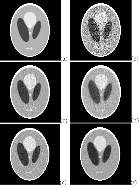
Transverse slice of the modified 3D Shepp-Logan phantom: (a) noise free image; (b) noisy image by FBP with the Ramp filter; (c) FBP image with the Hanning filter; (d) image reconstructed by the OSEM; (e) FBP image from the PWLS smoothed sinogram without KL transform using a penalty parameter 5×10⁻⁴; and (f) FBP image from the KL-PWLS filtered sinogram with a=500. The display window level is [500, 850].

Fig. 2.

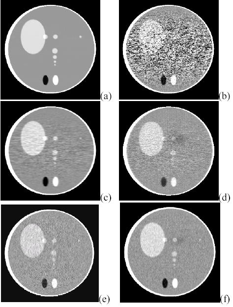
Sagittal slice of the modified 3D Shepp-Logan phantom: (a) noise free image; (b) noisy image by FBP with the Ramp filter; (c) FBP image with the Hanning filter; (d) image reconstructed by the OSEM; (e) FBP image from the PWLS smoothed sinogram without KL transform using a penalty parameter 5×10⁻⁴; and (f) FBP image from the KL-PWLS smoothed sinogram with a=500. The display window level is [500, 850].

Fig. 3.

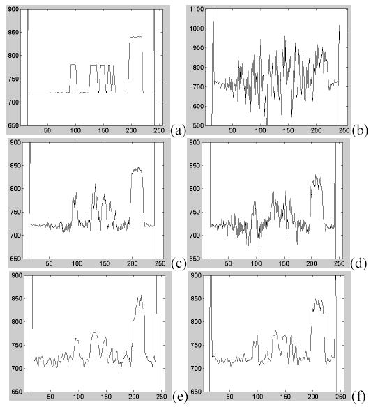
Vertical profiles drawn through the small objects of the sagittal images in Fig. 2.

In addition to the comparison to the well-known low-pass Hanning filter, the study was extended to include the well-established iterative OSEM (Ordered-Subsets Expectation-Maximization) reconstruction [11], as well as the PWLS minimization without KL transform. The ordered subsets were selected according to the geometrical symmetry of the detector system [12] with the number of projections in each subset equal to 8. The initial estimate was set as uniform, and the iterative process was terminated after initial convergence and before divergence. The result at the 4^th iteration is the best, by visual judgment, as compared to those with less or more than four iterations, given the know phantom.

Figure 1 shows a transverse slice of the phantom and the reconstructed images by different noise filtering or suppressing methods. Figure 2 shows a sagittal slice of the phantom and the reconstructed images by different noise filtering or suppressing methods. It can be observed that the reconstructed image from the KL-PWLS filtered sinograms shows a noticeable noise suppression and resolution preservation. This observation can be confirmed by the profiles along the z-axis of the phantom as shown in Figure 3. The low-pass Hanning filter could not reach the KL-PWLS result by any choice of the cutoff frequency. The OSEM could not generate the same quality result of the KL-PWLS by any number of iterations. Less iteration generated lower resolution images. While higher iteration improved the resolution, but generated more noisy images. This comparison suggests that higher low-contrast detectability could be achieved by the presented KL-PWLS scheme as compared to the optimized Hanning filter and iterative OSEM reconstruction.

We also present FBP results from smoothed sinograms after minimization of a modified PWLS objective function without the KL transform, where the modification was made by extending the quadratic form penalty to include nearby pixels along the z-axis in the sinogram space and the minimization was achieved by using iterative Gaussian-Seidel updating strategy [13]. It can be observed from Figure 1(e), Figure 2(e) and Figure 3(e) that the results of PWLS without KL transform are generally better than those of Hanning filter and OSEM reconstruction. The results of PWLS without KL transform are somewhat different from the results of the KL-PWLS algorithm. The difference may be explained by the fact that in the KL-PWLS algorithm the correlation among different slices is considered by the KL transform while in the PWLS without KL transform the correlation is considered by the quadratic form penalty. This different performance due to the different treatment on the correlation by the KL-PWLS and the PWLS without KL transform is worth of further investigation. In the following of this paper, we will only focus on the comparison studies of the presented KL-PWLS algorithm with the well-established Hanning filter and OSEM reconstruction algorithm.

To quantitatively evaluate the performance of the presented KL-PWLS filtering scheme with comparison to the optimized Hanning filter and OSEM reconstruction, observer studies were performed using the ROC and HT merits.

A. ROC Study

One generally accepted method for evaluation of the performance of a medical imaging system or procedure is to evaluate the ability of an observer to detect an abnormality. By the observer study, a variety of pairs of true positive fraction (TPF) and false positive fraction (FPF) is generated as an observer changes the confidence threshold, and a ROC curve is then drawn or fitted from the obtained TPF and FPF [14]. Each ROC curve describes the inherent discrimination capacity of an imaging system or procedure. A common merit for comparing the ROC curves is the area under the curve (AUC) or A_Z. The filtering scheme which generates a larger AUC usually reflects a better detectability on abnormality.

To perform a ROC study, we carefully designed a low-contrast small lesion in the Shepp-Logan phantom where the parameters of the lesion in the phantom are listed in the last row of Table I. Figure 4(a) shows a transverse slice of the phantom that contains the lesion volume, as indicated by the “arrow” in the picture. The noise-free sinograms of the phantom with and without the lesion were computed, respectively, using the same configuration and/or procedure as described in Part III above. A total of 500 noisy realizations were generated from each of the two sets of noise-free sinograms by adding signal-dependent Gaussian noise with variance determined by equation (1). Then these noisy realizations were reconstructed by the OSEM algorithm and the FBP with different noise filters: the optimized Hanning filter and the KL-PWLS strategy, resulting in a total of 3,000 volumetric 256 cubic images. A typical reconstructed image slice of the phantom with lesion by different methods, respectively, is shown in Figure 4.

Fig. 4.

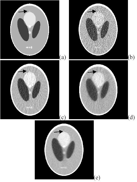
Transverse slice of the 3D Shepp-Logan phantom with a low-contrast small lesion: (a) noise free image; (b) noisy image by FBP with the Ramp filter; (c) FBP image with the optimized Hanning filter; (d) image reconstructed by the OSEM after 4 iterations; and (e) FBP image from the KL-PWLS filtered sinogram with a=500. The arrow in each image indicates the location of the lesion. The display window level is [500, 850].

ROC study was performed for two comparisons: (1) between the KL-PWLS noise filtering and the Hanning filter; and (2) between the KL-PWLS scheme and the OSEM reconstruction. In each comparison, two images reconstructed by two different methods respectively from the same noisy sinograms were presented in the same time for observers’ scoring. For each image, an observer was asked to select one of the five categories of confidence: (1) definitely or almost definitely negative, (2) probably negative, (3) possibly positive, (4) probably positive, and (5) definitely or almost definitely positive [14]. The scores were analyzed using the CLABROC code [15] and resulted in four pairs of FPF and TPF for each filtering method. Results for comparison of the KL-PWLS noise filtering and the Hanning filter were plotted in Figure 5. The fitted ROC curves by the binormal model were also drawn in the figure. The area under the ROC curve is 0.963 for the KL-PWLS scheme and 0.888 for the Hanning filter. The one-tailed p-value is less than 0.005, which indicates that the difference between these two filtering schemes is statistically significant. Figure 6 shows the comparison results between the KL-PWLS scheme and the OSEM reconstruction. The area under the fitted ROC curve is 0.950 for the KL-PWLS scheme and 0.871 for the OSEM reconstruction. The one-tailed p-value is less than 0.005, indicating a statistically significant difference between these two methods.

Fig. 5.

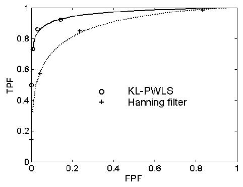
Results of ROC evaluation and the fitted ROC curves of the binormal model. The solid line (and circles) represents the result of the KL-PWLS scheme and the dashed line (and crosses) stands for the result of the Hanning filter.

Fig. 6.

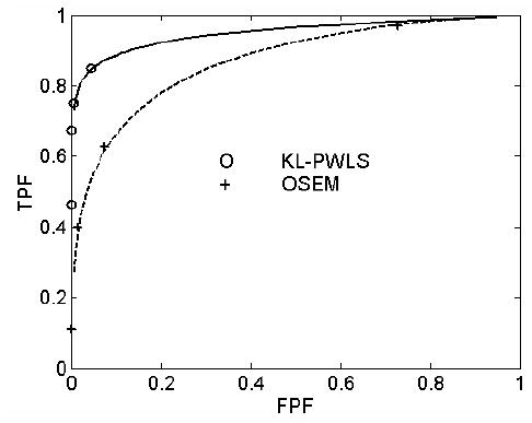
Results of ROC evaluation and the fitted ROC curves of the binormal model. The solid line (and circles) represents the result of the KL-PWLS filtering scheme and the dashed line (and crosses) stands for the result of the OSEM algorithm.

In the above two ROC comparisons, the AUCs for the KL-PWLS scheme are slightly different from each other, reflecting the variation of observer’s performance over different time periods and different image-review settings. This variation is dramatically smaller than the difference between the KL-PWLS and the low-pass Hanning filter or the OSEM algorithm. Both the optimized Hanning filter and OSEM algorithm performed similarly in detecting the small abnormality in this low contrast environment.

B. Hotelling Trace Calculation

Computer-based observers mimicking human observers have been proposed to alleviate the need for observers’ interactions. One of these methods is the Hotelling observer for comparison of two imaging systems or procedures. In this method, the Hotelling trace [16], which is a measure of object class separability based on the first and second-order statistics, is used to evaluate the ability of a system in separating between classes. In fact, Fiete et al. [17] found that the HT correlates with human performance in liver defect detection and Wollenweber et al. [18] recently implemented the HT to evaluate the potential increase in defect detection in myocardial SPECT (single photon emission computed tomography) using high-resolution fan-beam collimator versus parallel-hole collimation. Several other applications have also been reported recently. For example, Han et al. [19] employed the HT calculation to measure the gain by varying focal fan-beam collimation over parallel-hole geometry in quantitative chest SPECT. Li et al. [20] applied the HT calculation to measure the similarity of iterative and analytical reconstruction of quantitative brain SPECT considering Poisson noise, nonuniform attenuation (absorption and scatter) and point spread function (PSF) variation. All these computer-based observer studies concur with the human ROC results.

The mathematical formalism for calculating the HT is outlined below. For M classes of images, random samples are drawn to calculate the HT. Let f_j,m be the j-th sample from class m, where m = 1,2,…, M and j=1,2, …, N_m, and N_m be the number of samples from class M. Also suppose that the probability density function of occurrence for the sample f_j,m is p_j,m. Define the inter-class scatter matrix S₁ and intra-class scatter matrix S₂ as follows:

$$S_1=\sum _{m=1}^M{p}_m({\overline{f}}_m-\overline{f}){({\overline{f}}_m-\overline{f})}^T$$ (10)

$$S_2=\sum _{m=1}^M{p}_m{C}_m$$ (11)

where

$$p_k=\sum _{j=1}^{N_m}{p}_{j,m}$$ (12)

is the a priori probability of occurrence of class k in all the samples;

$${\overline{f}}_k=\sum _{j=1}^{N_k}\frac{p_{j,k}}{p_k}{f}_{j,k}$$ (13)

is the mean image of class k;

$$\overline{f}=\sum _{j=1}^{N_k}{p}_k{\overline{f}}_k$$ (14)

is the mean of mean class images which is also the grand mean of all images; and

$$C_k=\sum _{j=1}^{N_k}\frac{p_{j,k}}{p_k}(f_{j,k}-{\overline{f}}_k){(f_{j,k}-{\overline{f}}_k)}^T$$ (15)

is the covariance matrix for the k-th class. With the above definitions, the HT is defined as:

$$J=tr\mathrm{\hspace{0.17em} }(S_2^{-1}{S}_1).$$ (16)

From the above definitions, the dimension of the scatter matrices is equal to the number of pixels (or voxels) in the image, which is huge. The main difficulty in calculating J value therefore lies in inverting the matrix S₂. Matrix S₂ is singular if the number of sample images is less than the number of voxels in the image. The requirement that the number of sample images be not less than the number of voxels in the image would consume too much disk storage or computer memory. Abbey et al. [21] suggested the use of subsets of the images, instead of the whole images, to reduce the amount of required space or data to calculate the J value.

The HT value J was then calculated using the above formalism with the images reconstructed in the previous section. The two classes of reconstructed images are those with and without the lesion respectively. In the first HT calculation the images of the presented KL-PWLS filtering scheme was used. In the second HT calculation the images of the low-pass Hanning filter was used. In the third HT calculation the images of the OSEM reconstruction was used. Different sizes of ROI (region of interest) containing the lesion were chosen for the calculation of the HT, and the results are shown in Table II. As shown in the table, the HT J values of the KL-PWLS filtering scheme are larger than the values of the Hanning filter and OSEM algorithm no matter what size of ROI was chosen. These results concur with the ROC measures and indicate that the KL-PWLS scheme can outperform the optimized Hanning filter and the OSEM reconstruction in terms of low-contrast lesion detectability.

Table II.

Hotelling trace J calculation for FBP reconstructed images by KL-PWLS, OSEM and Hanning filter

ROI (pixels x pixels)	15 x 15	20 x 20	25 x 25
KL-PWLS	6.32	8.97	15.9
Hanning	4.03	6.03	10.8
OSEM	2.69	4.14	7.09

IV. Discussion and Conclusion

In this study, we presented a KL domain PWLS scheme to treat the noise in low-dose single-slice HCT sinograms. The presented scheme modeled the noise properties (of the first and second statistical moments) of the low-dose CT sinograms and considered the non-stationary PWLS weights or variance. The solution of the KL-PWLS scheme was calculated analytically. The KL transform was first applied along the neighboring sinograms to utilize the correlative information along the axial direction of the helical sampling. Then the PWLS objective function was minimized adaptively to estimate the ideal projection data for each KL component.

To achieve direct or analytical solution for maximum efficiency in computation, the penalty weights along the angular direction was set to zero which means only penalty among neighboring detector bins was considered in each KL component. One could consider the penalty along the angular direction by setting the weighting value w_im in equation (8) for those two nearest neighbors along the angular direction to be non-zero. By this design, the sets of linear equation (9) will no longer be tri-diagonal so that a direct analytical solution through the LU decomposition may not be tractable because a huge memory space is needed in the LU decomposition procedure. However, the KL-PWLS solution can still be calculated efficiently by iterative strategy, such as the iterated conditional mode (ICM) algorithm [6]. The effect of different penalties on the KL-PWLS solution by either the direct KL analysis or an indirect a priori constraint in the sinogram space needs further investigation.

The KL-PWLS minimization were executed on a PC with Pentium IV processor of 2.4 GHz CPU and 1.5 GB RAM. It took 140 seconds for the KL-PWLS minimization procedure to filter the whole sinogram volume of 512×512×170 array size. The computational efficiency can be further improved by parallel computing the independent KL components. The iterative OSEM reconstruction from the noisy sinogram volume to 256 cubic image array consumed 5,355 seconds for 4 iterations.

Quantitative evaluation by ROC study and HT calculation revealed that the presented KL-PWLS scheme can outperform the iterative OSEM reconstruction with an optimal number of iterations and the low-pass Hanning filter with an optimal cutoff frequency in terms of lesion detectability in low-contrast environment. The above results can be explained as follows. The low-pass Hanning filter is spatially invariant and indistinguishably smoothes the noise and edge information. Therefore, it reduces the noise level at the cost of proportional loss of the edge details. Although the OSEM algorithm weights optimally the ratio of the measured datum and the reprojected datum by the corresponding projection matrix element, it still fits each (assumed independent) measured datum and does not have a noise control mechanism. It has been well-recognized that a penalty is needed for a Bayesian iterative reconstruction [13]. For example, Sukovic et al. [22] explored PWLS reconstruction for dual-energy X-ray CT. Elbakri et al. [23] investigated an iterative algorithm to maximize a penalized-likelihood function, which incorporates polyenergetic nature of the X-ray source, for CT image reconstruction. Thibault et al. [24] extended the iterative algorithm to reconstruct HCT images.

It was shown in [24] that penalized iterative reconstruction methods may offer a better image quality as compared to the conventional FBP reconstruction (using a low-pass or other filters). This gain by the penalty is expected. However, for all of the fully iterative image reconstruction methods, the minimization of their objective functions in the image domain can be computationally intensive for CT applications of large volume datasets because the reprojection and backprojection cycle through the image domain is involved and the reprojection and backprojection cycle is very time consuming. The presented KL-PWLS scheme also minimizes a penalized cost function, but in the sinogram space by an analytical means for computing efficiency. Modeling the same data statistics by both iterative means in the image domain and analytical means in the sinogram space for quantitative SPECT application has shown a similar reconstruction quality, but at significantly different speeds [20, 25]. Such comparison study for CT application is an interesting research topic and is currently under progress. Furthermore, iterative calculation of a penalized cost function in the sinogram space can also be computationally efficient [6, 26–28], and is also worthy for further investigation.

References

- 1.Jung K, Lee K, Kim S, Kim T, Pyeun Y, Lee J. “Low-dose, volumetric helical CT: image quality, radiation dose, and usefulness for evaluation of bronchiectasis”. Invest Radiology. 2000;35:557–563. doi: 10.1097/00004424-200009000-00007. [DOI] [PubMed] [Google Scholar]
- 2.Hsieh J. “Nonstationary noise characteristics of the helical scan and its impact on image quality and artifacts”. Medical Physics. 1997;24:1375–1384. doi: 10.1118/1.598026. [DOI] [PubMed] [Google Scholar]
- 3.Lu H, Li X, Liang Z. “Analytical noise treatment for low-dose CT projection data by penalized weighted least-square smoothing in the K-L domain”. SPIE Medical Imaging. 2002;4682:146–152. [Google Scholar]
- 4.H. Lu, I. Hsiao, X. Li, and Z. Liang, “Noise properties of low-dose CT projections and noise treatment by scale transformations”, Conf. Record IEEE NSS-MIC, in CD-ROM, 2001.
- 5.Li T, Wang J, Wen J, Li X, Lu H, Hsieh J, Liang Z. “SNR-weighted sinogram smoothing with improved noise-resolution properties for low-dose X-ray computed tomography”. SPIE Medical Imaging. 2004;5370:2058–2066. [Google Scholar]
- 6.Li T, Li X, Wang J, Wen J, Lu H, Hsieh J, Liang Z. “Nonlinear sinogram smoothing for low-dose X-ray CT”. IEEE Trans Nuclear Science. 2004;51:2505–2513. [Google Scholar]
- 7.Wernick MN, Infusino EJ, Miloševiz M. “Fast spatiotemporal image reconstruction for dynamic PET”. IEEE Trans Medical Imaging. 1999;18:185–195. doi: 10.1109/42.764885. [DOI] [PubMed] [Google Scholar]
- 8.W.H. Press, S.A. Teukolsky, W.T. Vetterling, and B.P. Flannnery, Numerical Recipes in C: The art of scientific computing. Second Edition, Cambridge University Press, pp. 50–51, 1992.
- 9.Crawford CR, King KF. “Computed tomography scanning with simultaneous patient translation”. Medical Physics. 1990;17:967–981. doi: 10.1118/1.596464. [DOI] [PubMed] [Google Scholar]
- 10.Chiarot CB, Siewerdsen JH, Haycocks T, Moseley DJ, Jaffray DA. “An innovative phantom for quantitative and qualitative investigation of advanced x-ray imaging technologies”. Phys Med Biol. 2005;50:N287–N297. doi: 10.1088/0031-9155/50/21/N01. [DOI] [PubMed] [Google Scholar]
- 11.Hudson HM, Larkin RS. “Accelerated image reconstruction using ordered subsets of projection data”. IEEE Trans Medical Imaging. 1994;13:601–609. doi: 10.1109/42.363108. [DOI] [PubMed] [Google Scholar]
- 12.Han G, Liang Z. “A fast projector and back-projector for SPECT with varying focal-length fan-beam collimators”. J Nuclear Medicine. 2000;41:194. [Google Scholar]
- 13.Sauer K, Bouman C. “A local update strategy for iterative reconstruction from projections”. IEEE Trans Signal Processing. 1993;41:534–548. [Google Scholar]
- 14.Metz CE. “ROC methodology in radiological imaging”. Invest Radiology. 1986;21:720–733. doi: 10.1097/00004424-198609000-00009. [DOI] [PubMed] [Google Scholar]
- 15.Metz CE, Wang P-L, Kroman HB. “A new approach for testing the significance of differences between ROC curves measured from correlated data”. Information Processing in Medical Imaging. 1984:432–445. [Google Scholar]
- 16.Hotelling H. “The generalization of student’s ratio”. Annals Math Stat. 1931;2:360–378. [Google Scholar]
- 17.Fiete RD, Barrett HH, Smith WE, Myers KJ. “Hotelling trace criterion and its correlation with human-observer performance”. J Opt Soc Amer A. 1987;4:945–953. doi: 10.1364/josaa.4.000945. [DOI] [PubMed] [Google Scholar]
- 18.Wollenweber SD, Tsui BMW, Lalush DS, Frey EC, Gullberg GT. “Evaluation of myocardial defect detection between parallel-hole and fan-beam SPECT using the Hotelling trace”. IEEE Trans Nuclear Science. 1998;45:2205–2210. [Google Scholar]
- 19.Han G, Zhu W, Liang Z. “Gain of varying focal-length fan-beam collimator for cardiac SPECT by ROC, Hotelling trace, and bias-variance measures,”. J Nuclear Medicine. 2001;42:7. [Google Scholar]
- 20.Li T, Wen J, Liang Z. “Performance evaluation of analytical- and iterative-based quantitative brain SPECT reconstruction with fan-beam collimation by both Human (ROC) and computer (CHO) observers, as well as bias-variance plot”. J Nuclear Medicine. 2004;45(5):46. [Google Scholar]
- 21.Abbey CK, Barrett HH, Eckstein MP. “Practical issues and methodology in assessment of image quality using model observers”. SPIE Medical Imaging. 1997;3032:182–194. [Google Scholar]
- 22.Sukovic P, Clinthorne NH. “Penalized weighted least-squares image reconstruction for dual energy X-ray transmission tomography”. IEEE Trans Medical Imaging. 2000;19:1075–1081. doi: 10.1109/42.896783. [DOI] [PubMed] [Google Scholar]
- 23.Elbakri IA, Fessler JA. “Statistical image reconstruction for polyenergetic X-ray computed tomography”. IEEE Trans Medical Imaging. 2002;21:89–99. doi: 10.1109/42.993128. [DOI] [PubMed] [Google Scholar]
- 24.J. Thibault, K. Sauer, C. Bouman, and J. Hsieh, “High quality iterative image reconstruction for multi-slice helical CT”, International Conference on Fully 3D Reconstruction in Radiology and Nuclear Medicine, Saint Malo, 2003.
- 25.Li T, Wen J, Han G, Lu H, Liang Z. “Evaluation of an efficient compensation method for quantitative fan-beam brain SPECT reconstruction,”. IEEE Trans Medical Imaging. 2005;24:170–179. doi: 10.1109/tmi.2004.839365. [DOI] [PubMed] [Google Scholar]
- 26.P.J. La Rivière, “Reduction of noise-induced streaking artifacts in X-ray CT through penalized-likelihood sinogram smoothing”, Conf. Record IEEE NSS and MIC, in CD-ROM, 2003.
- 27.P.J. La Rivière and D.M. Billmire, “Reduction of noise-induced streak artifacts in X-ray computed tomography through spline-based penalized-likelihood sinogram smoothing”, IEEE Trans. Medical Imaging, vol. 24, pp. 105–111, 2005. [DOI] [PubMed]
- 28.La Rivière PJ. “Penalized-likelihood sinogram smoothing for low-dose CT”. Medical Physics. 2005;32:1676–1683. doi: 10.1118/1.1915015. [DOI] [PubMed] [Google Scholar]