The Affected-/Discordant-Sib-Pair Design Can Guarantee Validity of Multipoint Model-Free Linkage Analysis of Incomplete Pedigrees When There Is Marker-Marker Disequilibrium

Abstract

Genomewide linkage studies are tending toward the use of single-nucleotide polymorphisms (SNPs) as the markers of choice. However, linkage disequilibrium (LD) between tightly linked SNPs violates the fundamental assumption of linkage equilibrium (LE) between markers that underlies most multipoint calculation algorithms currently available, and this leads to inflated affected-relative-pair allele-sharing statistics when founders’ multilocus genotypes are unknown. In this study, we investigate the impact that the degree of LD, marker allele frequency, and association type have on estimating the probabilities of sharing alleles identical by descent in multipoint calculations and hence on type I error rates of different sib-pair linkage approaches that assume LE. We show that marker-marker LD does not inflate type I error rates of affected sib pair (ASP) statistics in the whole parameter space, and that, in any case, discordant sib pairs (DSPs) can be used to control for marker-marker LD in ASPs. We advocate the ASP/DSP design with appropriate sib-pair statistics that test the difference in allele sharing between ASPs and DSPs.

A universal assumption in multipoint linkage analysis has been that the markers are in linkage equilibrium (LE).^1,2 This assumption is reasonable and feasible for maps of sparse microsatellite markers. However, this assumption starts to break down as we look at denser and denser SNP maps; not allowing for the linkage disequilibrium (LD) will lead to incorrect inferences of the haplotype frequencies of a cluster of tightly linked markers.^3,4 In linkage analysis, if the marker-marker LD is not taken into account, the founder diplotype frequencies are obtained from the population allele frequencies by assuming Hardy-Weinberg proportions at each locus and LE across loci. When the founder genotypes are unknown, the use of misspecified haplotype frequencies—analogous to that of misspecified single-marker allele frequencies—is a potential source of error. Huang et al.⁴ showed that ignoring LD between markers can lead to overestimated sharing of alleles identical by descent (IBD) among affected siblings in multipoint IBD (MIBD) probability calculations. The excessive MIBD sharing would then generate false-positive evidence of linkage in affected sib pair (ASP) analysis, which has been demonstrated in both simulation studies^4–7 and real data analysis.⁸ Several approaches have been proposed to control the type I error rate to a given level when markers are in LD. Some researchers have suggested using only markers in low LD for multipoint linkage analysis by deleting those in high LD.⁹ Linkage software that organizes markers in LD into clusters and estimates unbiased haplotype frequencies has also been developed.¹⁰ Bacanu¹¹ proposed the multipoint-on-subsets statistics, in which the markers are partitioned into interlacing but nonoverlapping subsets. The impact of marker-marker LD on multipoint model-free linkage analysis of pedigrees with missing founder genotypes depends on many factors, including the degree of LD (which depends on the type of LD measure), the linkage statistic, and the study design employed. Studies so far have not fully explored the parameter space or recommended designs when they come to the conclusion that marker-marker LD necessarily inflates the type I error rate in multipoint linkage analysis if founder genotypes are missing. In the current study, we systemically investigate the impact of degree of LD, marker allele frequencies, and association type (see below for the definition of this term) on estimation of the probabilities of sharing alleles MIBD and on type I error rate arising from different model-free linkage approaches under the assumption of LE. The main aims of this report are thus to address the following issues. (1) In what situations does marker-marker LD cause highly biased MIBD estimation? (2) In what situations does marker-marker LD inflate type I error rates for a set of popular ASP linkage methods? (3) What is the validity of different linkage statistics using designs that incorporate discordant sib pairs (DSPs) when there is marker-marker LD?

A principal assumption of model-free linkage analysis is that affected relative pairs tend to share more alleles IBD at the disease location than at other regions in the genome. Therefore, to study the impact of marker-marker LD on linkage, we first study theoretically its impact on estimation of the proportion of alleles shared MIBD. Without loss of generality, we consider only the case of independent sib pairs with two tightly linked diallelic markers, between which any recombination can be ignored. Two diallelic markers can lead to four possible haplotypes. Hence, there can be 10 phase-known genotypes for a random individual and 55 phase-known pairs of genotypes for a random sib pair. The proportion of haplotypes shared IBD by a random sib pair is calculated as follows: (1) we first calculate the population haplotype frequencies on the basis of the allele frequencies and the degree of LD; (2) assuming random mating, we calculate the probabilities of observing a sib pair with phase-known genotypes, denoted , where H denotes haplotype and 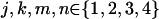; (3) we calculate the exact probabilities of haplotypes shared IBD by a sib pair, given phase-known genotypes, denoted 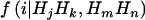, where , by using the Elston-Stewart algorithm^12,13; and, finally, (4) we calculate the expected proportion of haplotypes shared IBD between members of a random sib pair as , with the summation over j, k, m, and n. Because these two markers are assumed to be tightly linked, the estimated haplotype IBD sharing can be regarded as alleles shared MIBD for the two loci. When both 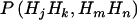and are calculated at the same level of LD, is an unbiased estimate of the haplotype (or allele) MIBD sharing; however, when one of them is calculated at LE and the other at LD, the haplotype frequencies used are inconsistent, and so the MIBD sharing is estimated with bias.

Using the method of calculation described above, we systematically study the impact of marker-marker LD on the estimation of the proportion of alleles shared MIBD, with the following parameter values. The degree of LD, measured by D′,¹⁴ takes on the values {0.0,0.4,0.8,1.0}. Because D′ depends on the allele frequencies,¹⁵ we vary the minor-allele frequencies over the range {0.1,0.3,0.5}. We constrain D′ to be nonnegative, so that “positive” association—that is, a positive value of D′—can occur between minor (or major) alleles at both loci, or between a minor allele at one locus and a major allele at the other locus. Therefore, we define association types between two loci as minor_p-minor_q (or, equivalently, major_p-major_q) and minor_p-major_q, where p and q denote the minor- or major-allele frequencies at the two loci, respectively. We consider four degrees of LD, D^′=0.0, 0.4, 0.8, and 1.0, for each of the following five association types: minor_0.1-minor_0.1, minor_0.3-minor_0.3, minor_0.5-minor_0.5, minor_0.1-major_0.9, and minor_0.3-major_0.7—in other words, we only consider the special association types minor_p-minor_p and minor_p-major_1−p. We also calculated the value of another popular measurement of LD, r², corresponding to the values of D′, p, and q. Note that when the association type is minor_p-minor_p, ; when the association is minor_p-major_1−p, r² cannot be 1.

Given the correct allele frequencies at each locus, the difference in haplotype frequencies between the situation where LE is assumed and the situation where LD is assumed varies according to the association type and degree of LD (table 1). The absolute value of the haplotype frequency difference between LE and LD is a monotonically increasing function of D′. For any haplotype, the more D′ increases, the further the frequency deviates from that of LE; this result holds under any association type. The degree of deviation is different for the different association types. When the association type is minor_p-minor_p, the deviations increase as p increases. The change in the absolute value of the deviation from D^′=0 to D^′=1 is 0.09, 0.21, and 0.25 when p=q=0.1, 0.3, and 0.5, respectively; however, when the association is minor_p-major_1−p, although the deviation again increases as p increases, the change in the absolute value of the deviation from D^′=0 to D^′=1 is only 0.01 when p=0.1 and is 0.09 when p=0.3. The expected probabilities of sharing 0, 1, and 2 alleles MIBD (denoted f₀, f₁, and f₂) between a random sib pair are 0.25, 0.5, and 0.25, respectively. The corresponding estimates under the assumption of LE when the true state is LD deviate from expectations in a manner that depends on the association type and degree of LD (table 2), which is consistent with the haplotype frequencies because misspecified haplotype frequencies lead directly to biased estimates of MIBD sharing. Under the association type minor_p-minor_p and given p, as D′ increases, f₀ decreases, while f₂ increases and f₁ remains relatively constant around 0.5, and thus the mean proportion of alleles shared MIBD (f₂+0.5×f₁) increases. This trend becomes more obvious as p increases—for example, when p increases from 0.1 to 0.5, f₂+0.5×f₁ increases from 0.507 to 0.518 at D^′=0.4 and from 0.530 to 0.615 at D^′=1.0. Under the association type minor_p-major_1−p, f₁ still remains relatively constant around 0.5, given any p; however, both f₀ and f₂ show different monotonic functional relationships with D′ when p takes on different values. When p=0.1, f₀ increases and f₂ decreases as D′ increases, but the extent of the increase and decrease is so small that f₂+0.5×f₁ is still close to 0.5. When p⩾0.2, f₀ decreases and f₂ increases, and thus f₂+0.5×f₁ increases as D′ increases. In summary, under the association type minor_p-minor_p, the mean proportion of alleles shared MIBD between a random sib pair estimated under the assumption of LE is inflated (>0.5) at any level of p, and the relative increase is >1% when D^′>0.2, or r²>0.04. Under the association type minor_p-major_1−p, the relative increase of estimated mean allele MIBD sharing is >1% only when p⩾0.3 and D^′⩾0.4, or r²>0.03.

Table 1. .

Estimated Haplotype Frequencies of Two Diallelic Markers under the Assumption of LE for Different Association Types and Degrees of LD

	Haplotype Frequency for D′ =
Association Type and Haplotypea	.0	.4	.8	1.0
minor0.1-minor0.1:
r2	.000	.160	.640	1.000
AB	.010	.046	.082	.100
Ab	.090	.054	.018	.000
aB	.090	.054	.018	.000
ab	.810	.846	.882	.900
minor0.3-minor0.3:
r2	.000	.160	.640	1.000
AB	.090	.174	.258	.300
Ab	.210	.126	.042	.000
aB	.210	.126	.042	.000
ab	.490	.574	.658	.700
minor0.5-minor0.5:
r2	.000	.160	.640	1.000
AB	.250	.350	.450	.500
Ab	.250	.150	.050	.000
aB	.250	.150	.050	.000
ab	.250	.350	.450	.500
minor0.1-major0.9:
r2	.000	.002	.008	.012
AB	.090	.094	.098	.100
Ab	.010	.006	.002	.000
aB	.810	.806	.802	.800
ab	.090	.094	.098	.100
minor0.3-major0.7:
r2	.000	.029	.118	.184
AB	.210	.246	.282	.300
Ab	.090	.054	.018	.000
aB	.490	.454	.418	.400
ab	.210	.246	.282	.300

^aFrequencies of alleles A and B correspond to the first and second allele frequencies in the association type.

Table 2. .

Probabilities of the Number of Haplotypes (or Alleles) Shared IBD (or MIBD) between Random Full Sibs, Estimated under the Assumption of LE^[Note]

	Value for D′ =
Association Type and Variable	.0	.4	.8	1.0
minor0.1-minor0.1:
r2	.000	.160	.640	1.000
f0	.250	.243	.230	.220
f1	.500	.500	.500	.500
f2	.250	.257	.270	.280
f2+0.5×f1	.500	.507	.520	.530
minor0.3-minor0.3:
r2	.000	.160	.640	1.000
f0	.250	.235	.193	.163
f1	.500	.500	.498	.493
f2	.250	.265	.308	.344
f2+0.5×f1	.500	.515	.558	.590
minor0.5-minor0.5:
r2	.000	.160	.640	1.000
f0	.250	.232	.179	.142
f1	.500	.501	.497	.486
f2	.250	.267	.324	.372
f2+0.5×f1	.500	.518	.573	.615
minor0.1-major0.9:
r2	.000	.002	.008	.012
f0	.250	.250	.251	.251
f1	.500	.500	.500	.500
f2	.250	.250	.249	.249
f2+0.5×f1	.500	.500	.499	.499
minor0.3-major0.7:
r2	.000	.029	.118	.184
f0	.250	.247	.240	.234
f1	.500	.501	.503	.504
f2	.250	.252	.258	.263
f2+0.5×f1	.500	.502	.509	.514

Note.— D′ is the true degree of LD. f₀, f₁, and f₂ are the expected probabilities of sharing 0, 1, and 2 alleles MIBD, respectively, and f₂+0.5×f₁ corresponds to the mean proportion of allele sharing IBD.

To determine the situations under which marker-marker LD inflates type I error rates for ASP linkage methods, we simulated two diallelic markers for the five association types at four different degrees of LD, as summarized in table 3. Nuclear families consisting of two parents and two children were simulated by first randomly assigning haplotypes to both parents on the basis of population haplotype frequencies and then segregating the haplotypes to each child according to Mendel’s law of segregation. We then deleted the parental data so that only sib-pair data were available. We specified the null hypothesis of no linkage between the marker and disease loci by assuming that no disease gene is segregating in the data—that is, a child’s disease affection status was assigned randomly. Samples consisting of 200 ASPs were simulated, and 10,000 replicate samples were generated under each of the 20 simulations. Assuming LE between the two markers and specifying that the recombination fraction between them is 0.001, we performed ASP linkage analysis by three different approaches: the mean test,¹⁶ a reparameterized maximum LOD score (MLS) method,^17,18 and the allele-sharing method under the “linear” model proposed by Kong and Cox,¹⁹ for which the test statistics are denoted T_ASP, MLS_ASP, and Z_lin-ASP, respectively. T_ASP was calculated using SIBPAL, and MLS_ASP was calculated using LODPAL; both these programs are included in the S.A.G.E. software suite version 5.2 (2006).²⁰ Z_lin-ASP was calculated using GENEHUNTER-PLUS.¹⁹ For all these statistics, at all levels of D′, we calculated the empirical type I error at a nominal .05 significance level as the proportion of the 10,000 replicates for which the P value was ⩽.05.

Table 3. .

Empirical Type I Error Rates at a Nominal .05 Significance Level for ASP Statistics under the Assumption of LE^[Note]

	Type I Error Rate for D′ =
Association Type and Method	.0	.4	.8	1.0
minor0.1-minor0.1:
r2	.000	.160	.640	1.000
TASP	.056	.133	.375	.554
MLSASP	.052	.171	.561	.796
Zlin-ASP	.053	.127	.263	.542
minor0.3-minor0.3:
r2	.000	.160	.640	1.000
TASP	.051	.162	.751	.978
MLSASP	.049	.185	.856	.996
Zlin-ASP	.051	.160	.749	.978
minor0.5-minor0.5:
r2	.000	.160	.640	1.000
TASP	.055	.149	.829	.996
MLSASP	.054	.159	.886	.999
Zlin-ASP	.054	.147	.829	.996
minor0.1-major0.9:
r2	.000	.002	.008	.012
TASP	.052	.050	.049	.047
MLSASP	.050	.044	.044	.042
Zlin-ASP	.050	.047	.047	.046
minor0.3-major0.7:
r2	.000	.029	.118	.184
TASP	.053	.057	.075	.096
MLSASP	.051	.056	.075	.098
Zlin-ASP	.052	.056	.074	.095

Note.— The sample comprises 200 independent ASPs.

For the ASP design, if calculated under the assumption of LE when the true state is LD, not all statistics show an inflated type I error rate, and the degree of inflation (if there is any) is consistent with the degree of deviation of the estimates of the proportion of alleles shared MIBD from expectation, which depends on the association type and allele frequencies (table 3). Under the association type minor_p-minor_p and given p, the type I error rates of all three statistics are well controlled at 0.05 when D^′=0. The error rates increase as D^′ increases, and this trend becomes more obvious as p increases—for example, for T_ASP, when p increases from 0.1 to 0.5, the error rate increases from 0.554 to 0.996 at D^′=1.0. Under the association type minor_p-major_1−p, the type I error rates of all three statistics are well controlled at 0.05 at all levels of D′ when p⩽0.2. When p>0.2, at any level of D^′>0, the error rates are much smaller, although inflated compared with those under the association type minor_p-minor_p—for example, for T_ASP when p=0.3 and D^′=1, the error rate is 0.096 under the association type minor_p-major_1−p and 0.978 under the association type minor_p-minor_p.

To study the ASP/DSP design, we simulated 100 ASPs, as described above, and 100 DSPs, by assigning one sib as affected and the other as unaffected. We also simulated samples of 200 sib pairs with the ratio ASPs:DSPs of 1:3 or 3:1 under the association type minor_0.5-minor_0.5 and with D^′=0.0 or 1.0. Again, 10,000 replicate samples were generated under each of the simulation settings. We performed linkage analyses on the ASPs and DSPs by three approaches: Haseman-Elston (HE) regression,²¹ an analogous MLS method that contrasts the allele sharing between ASPs and DSPs,²² and an analogous allele-sharing method under a linear model that contrasts the allele sharing between ASPs and DSPs,²³ for which the test statistics are denoted HE_ADSP, MLS_ADSP, and Z_lin-ADSP, respectively. HE_ADSP was calculated using SIBPAL, MLS_ADSP was calculated using LODPAL, and Z_lin-ADSP was calculated using GENEHUNTER++sad.²³ Because MLS_ADSP does not have an explicit asymptotic distribution, as do the other two statistics, we determined a cutoff value c, such that when D^′=0.0, and then calculated the empirical type I error rate in cases of D^′⩾0.2 by 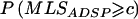. Note that HE regression can be used for the linkage analysis of any quantitative trait, including a binary trait that takes on one of only two values, 0 and 1. When the squared sib-pair difference—0 for concordant pairs and 1 for discordant pairs—is regressed on an estimate of the mean proportion of alleles shared IBD, and a one-sided test for the regression coefficient is performed, this essentially tests whether the mean proportion of alleles shared IBD is greater for concordant pairs than for DSPs²⁴ (see appendix A for a mathematical proof). This is another version of the mean test but is for an ASP/DSP design, as proposed by Blackwelder and Elston,¹⁶ and was applied soon after the HE method was first developed.²⁵ Although Z_lin-ADSP also tests the difference in the mean proportion of alleles shared IBD between ASPs and DSPs, it performs the comparison between ASPs and DSPs within each family and then takes a weighted average over all families.²³ In the case of HE regression, we should expect no change in type I error rate when testing the equality of IBD sharing between the two groups, because the DSPs form an appropriate control group. Bias will occur only if there is a confounder present such that, under the null hypothesis, the IBD sharing is different between ASPs and DSPs.

As confirmed in table 4, none of these statistics, if calculated under the assumption of LE when the true state is LD, with equal proportions of ASPs and DSPs, shows an inflated type I error rate. As might be expected, for the design with unequal proportions of ASPs and DSPs, if calculated under the assumption of LE when the true state is LD, both HE_ADSP and MLS_ADSP still control the type I error rate at 0.05. However, Z_lin-ADSP compares the mean proportions of alleles shared IBD between ASPs and DSPs within each family and then takes a weighted average over all families. Thus, compared with HE_ADSP and MLS_ADSP, it requires the presence of both ASPs and DSPs within each family; otherwise, it will be biased unless there are equal proportions of independent ASPs and DSPs. It is conservative when the ratio ASP:DSP is <1 and liberal when the ratio is >1 (table 5).

Table 4. .

Empirical Type I Error Rates at a Nominal .05 Significance Level for ASP/DSP Statistics under the Assumption of LE^[Note]

	Type I Error Rate at D′ =
Association Type and Method	.0	.4	.8	1.0
minor0.1-minor0.1:
r2	.000	.160	.640	1.000
HEADSP	.049	.052	.054	.050
MLSADSP	…	.048	.045	.051
Zlin-ADSP	.050	.052	.053	.049
minor0.3-minor0.3:
r2	.000	.160	.640	1.000
HEADSP	.051	.049	.050	.047
MLSADSP	…	.050	.051	.052
Zlin-ADSP	.051	.049	.047	.042
minor0.5-minor0.5:
r2	.000	.160	.640	1.000
HEADSP	.047	.051	.049	.051
MLSADSP	…	.049	.049	.047
Zlin-ADSP	.048	.051	.046	.043
minor0.1-major0.9:
r2	.000	.002	.008	.012
HEADSP	.053	.049	.051	.050
MLSADSP	…	.052	.055	.051
Zlin-ADSP	.050	.050	.052	.051
minor0.3-major0.7:
r2	.000	.029	.118	.184
HEADSP	.054	.049	.053	.046
MLSADSP	…	.047	.043	.048
Zlin-ADSP	.054	.049	.053	.046

Note.— The sample comprises 100 independent ASPs and 100 independent DSPs.

Table 5. .

Empirical Type I Error Rates at a Nominal .05 Significance Level for ASP/DSP Statistics under the Assumption of LE

	Type I Error Rate for D′ =
Ratio of ASPs:DSPs and Method	.0	1.0a
1:3
HEADSP	.052	.051
MLSADSP	…	.051
Zlin-ADSP	.053	.000
3:1
HEADSP	.052	.053
MLSADSP	…	.044
Zlin-ADSP	.052	.706

^aThe association type is minor_0.5-minor_0.5.

Model-free linkage analyses test the correlation between trait similarity and allele sharing between family members, and there are various statistics for the different study designs, each with its special assumptions. For sibship data and a dichotomous trait, Blackwelder and Elston¹⁶ showed that, for most rare-disease models, the most efficient study design is to sample ASPs, and the mean test is then the most powerful. However, they clearly stated one of the necessary assumptions: “In the absence of linkage, the expected proportions of sib pairs with 0, 1, and 2 marker alleles IBD are 1/4, 1/2 and 1/4, respectively, regardless of the sibs’ disease status.”^16(p86) This assumption is required for the validity of all statistics based on the ASP design. When marker-marker LD is not properly taken into account, this assumption is violated and all ASP statistics become invalid. Similarly, this assumption will also be violated when there is transmission-ratio distortion of the markers, again leading to invalidity of all ASP statistics. It has been suggested that DSPs should also be recruited, to check for transmission disequilibrium and to serve as a control group in sib-pair linkage studies.^16,22,23,26 With DSPs as controls, we can test the difference in allele sharing between ASPs and DSPs, and thus the above assumption is no longer required. For HE_ADSP, the estimates for the mean proportion of alleles shared IBD are inflated for both ASPs and DSPs, and thus the slope of the regression line is not significantly different from zero, which is the same as when the true state is LE. HE_ADSP is essentially a two-sample t test, whereas MLS_ADSP performs the comparison in a likelihood-ratio fashion.

Abecasis and Wigginton¹⁰ modeled marker-marker LD in a two-step approach by first clustering markers in LD and estimating the haplotype frequencies and then performing multipoint analysis based on the new composite markers. Compared with our proposition of using an ASP/DSP design to overcome issues arising from marker-marker LD, this approach corrects for the marker-marker LD when the allele sharing is calculated and thus can be employed for further multipoint analysis of all types. However, caution should be taken in using this approach, because it also has some potential problems: organizing markers into clusters is subjective, assuming no recombination within clusters discards part of the data, and specifying intercluster distance is subjective. Also note that this approach is not efficient when founder genotypes are available, because marker-marker LD causes problems only when founder genotypes are unknown. Although this approach provides one solution to the problem of marker-marker LD, we anticipate that a method will eventually be found to model marker-marker LD in multipoint analysis in a one-step fashion.

In summary, a linkage study with only ASPs is analogous to an epidemiological study with only cases, which can lead to spurious results. Although the ASP/DSP design is not as powerful as the ASP design, as shown by Blackwelder and Elston,¹⁶ its general validity should take precedence, and we advocate the ASP/DSP design to control for transmission disequilibrium caused either by biological processes, such as meiotic drive, or by computational complexity, such as marker-marker LD.

Appendix A: HE Method

The HE method tests whether the mean proportion of alleles shared IBD is greater for concordant pairs than for DSPs. The HE regression model can be written as 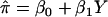, where is the estimated proportion of alleles shared IBD, Y is the squared trait difference for a pair of sibs, β₀ is the intercept, and β₁ is the slope. Note that we can exchange and Y in the original HE regression model because the t statistic for slope is invariant with respect to this interchange.²⁷ We test linkage by testing the hypotheses β₁=0 versus β₁<0. In the mean test (a two-sample t test), we test the hypotheses versus , where the subscript C denotes concordant sib pairs and D denotes discordant sib pairs. To prove the equivalence of these two tests under the null hypothesis of no linkage, we simply need to prove that their test statistics are identical.

Assume and let c and d denote the number of concordant and discordant sib pairs, respectively. The test statistic for the HE regression is

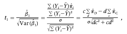which follows the t_c+d-2 distribution. Under the assumption 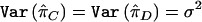, the test statistic for the mean test is

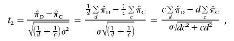which similarly follows the t_c+d-2 distribution. Therefore, these two statistics are identical under the null hypothesis of no linkage.

References

- 1.Lathrop GM, Lalouel JM, Julier C, Ott J (1984) Strategies for multilocus linkage analysis in humans. Proc Natl Acad Sci USA 81:3443–3446 10.1073/pnas.81.11.3443 [DOI] [PMC free article] [PubMed] [Google Scholar]
- 2.Lander ES, Green P (1987) Construction of multilocus genetic linkage maps in humans. Proc Natl Acad Sci USA 84:2363–2367 10.1073/pnas.84.8.2363 [DOI] [PMC free article] [PubMed] [Google Scholar]
- 3.Browning BL, Brashear DL, Butler AA, Cyr DD, Harris EC, Nelsen AJ, Yarnall DP, Ehm MG, Wagner MJ (2004) Linkage analysis using single nucleotide polymorphisms. Hum Hered 57:220–227 10.1159/000081449 [DOI] [PubMed] [Google Scholar]
- 4.Huang Q, Shete S, Amos CI (2004) Ignoring linkage disequilibrium among tightly linked markers induces false-positive evidence of linkage for affected sib pair analysis. Am J Hum Genet 75:1106–1112 [DOI] [PMC free article] [PubMed] [Google Scholar]
- 5.Huang Q, Shete S, Swartz M, Amos CI (2005) Examining the effect of linkage disequilibrium on multipoint linkage analysis. BMC Genet Suppl 1 6:S83 10.1186/1471-2156-6-S1-S83 [DOI] [PMC free article] [PubMed] [Google Scholar]
- 6.Boyles AL, Scott WK, Martin ER, Schmidt S, Li YJ, Ashley-Koch A, Bass MP, Schmidt M, Pericak-Vance MA, Speer MC, Hauser ER (2005) Linkage disequilibrium inflates type I error rates in multipoint linkage analysis when parental genotypes are missing. Hum Hered 59:220–227 10.1159/000087122 [DOI] [PMC free article] [PubMed] [Google Scholar]
- 7.Levinson DF, Holmans P (2005) The effect of linkage disequilibrium on linkage analysis of incomplete pedigrees. BMC Genet Suppl 1 6:S6 10.1186/1471-2156-6-S1-S6 [DOI] [PMC free article] [PubMed] [Google Scholar]
- 8.Schaid DJ, Guenther JC, Christensen GB, Hebbring S, Rosenow C, Hilker CA, McDonnell SK, Cunningham JM, Slager SL, Blute ML, Thibodeau SN (2004) Comparison of microsatellites versus single-nucleotide polymorphisms in a genome linkage screen for prostate cancer–susceptibility loci. Am J Hum Genet 75:948–965 [DOI] [PMC free article] [PubMed] [Google Scholar]
- 9.Webb EL, Sellick GS, Houlston RS (2005) SNPLINK: multipoint linkage analysis of densely distributed SNP data incorporating automated linkage disequilibrium removal. Bioinformatics 21:3060–3061 10.1093/bioinformatics/bti449 [DOI] [PubMed] [Google Scholar]
- 10.Abecasis GR, Wigginton JE (2005) Handling marker-marker linkage disequilibrium: pedigree analysis with clustered markers. Am J Hum Genet 77:754–767 [DOI] [PMC free article] [PubMed] [Google Scholar]
- 11.Bacanu SA (2005) Multipoint linkage analysis for a very dense set of markers. Genet Epidemiol 29:195–203 10.1002/gepi.20089 [DOI] [PubMed] [Google Scholar]
- 12.Elston RC, Stewart J (1971) A general model for the genetic analysis of pedigree data. Hum Hered 21:523–542 [DOI] [PubMed] [Google Scholar]
- 13.Boehnke M (1991) Allele frequency estimation from data on relatives. Am J Hum Genet 48:22–25 [PMC free article] [PubMed] [Google Scholar]
- 14.Lewontin RC (1964) The interaction of selection and linkage. I. General considerations; heterotic models. Genetics 49:49–67 [DOI] [PMC free article] [PubMed] [Google Scholar]
- 15.Lewontin RC (1988) On measures of gametic disequilibrium. Genetics 120:849–852 [DOI] [PMC free article] [PubMed] [Google Scholar]
- 16.Blackwelder WC, Elston RC (1985) A comparison of sib-pair linkage tests for disease susceptibility loci. Genet Epidemiol 2:85–97 10.1002/gepi.1370020109 [DOI] [PubMed] [Google Scholar]
- 17.Olson JM (1999) A general conditional-logistic model for affected-relative-pair linkage studies. Am J Hum Genet 65:1760–1769 [DOI] [PMC free article] [PubMed] [Google Scholar]
- 18.Goddard KA, Witte JS, Suarez BK, Catalona WJ, Olson JM (2001) Model-free linkage analysis with covariates confirms linkage of prostate cancer to chromosomes 1 and 4. Am J Hum Genet 68:1197–1206 [DOI] [PMC free article] [PubMed] [Google Scholar]
- 19.Kong A, Cox NJ (1997) Allele-sharing models: LOD scores and accurate linkage tests. Am J Hum Genet 61:1179–1188 [DOI] [PMC free article] [PubMed] [Google Scholar]
- 20.S.A.G.E. (2006) Statistical analysis for genetic epidemiology 5.2. (http://darwin.case.edu/sage/)
- 21.Haseman JK, Elston RC (1972) The investigation of linkage between a quantitative trait and a marker locus. Behav Genet 2:3–19 10.1007/BF01066731 [DOI] [PubMed] [Google Scholar]
- 22.Shih PY, Wang T, Xing C, Sinha M, Song Y, Elston RC (2005) Linkage analysis of alcohol dependence using both affected and discordant sib pairs. BMC Genet Suppl 1 6:S36 10.1186/1471-2156-6-S1-S36 [DOI] [PMC free article] [PubMed] [Google Scholar]
- 23.Lemire M, Roslin NM, Laprise C, Hudson TJ, Morgan K (2004) Transmission-ratio distortion and allele sharing in affected sib pairs: a new linkage statistic with reduced bias, with application to chromosome 6q25.3. Am J Hum Genet 75:571–586 [DOI] [PMC free article] [PubMed] [Google Scholar]
- 24.Elston RC, Song D, Iyengar SK (2005) Mathematical assumptions versus biological reality: myths in affected sib pair linkage analysis. Am J Hum Genet 76:152–156 [DOI] [PMC free article] [PubMed] [Google Scholar]
- 25.Elston RC, Kringlen E, Namboodiri KK (1973) Possible linkage relationships between certain blood groups and schizophrenia or other psychoses. Behav Genet 3:101–106 10.1007/BF01067650 [DOI] [PubMed] [Google Scholar]
- 26.Elston RC, Guo X, Williams LV (1996) Two-stage global search designs for linkage analysis using pairs of affected relatives. Genet Epidemiol 13:535–558 [DOI] [PubMed] [Google Scholar]
- 27.Schaid DJ, Olson JM, Gauderman WJ, Elston RC (2003) Regression models for linkage: issues of traits, covariates, heterogeneity, and interaction. Hum Hered 55:86–96 10.1159/000072313 [DOI] [PubMed] [Google Scholar]