A Coalescence-Guided Hierarchical Bayesian Method for Haplotype Inference

Abstract

Haplotype inference from phase-ambiguous multilocus genotype data is an important task for both disease-gene mapping and studies of human evolution. We report a novel haplotype-inference method based on a coalescence-guided hierarchical Bayes model. In this model, a hierarchical structure is imposed on the prior haplotype frequency distributions to capture the similarities among modern-day haplotypes attributable to their common ancestry. As a consequence, the model both allows distinct haplotypes to have different a priori probabilities according to the inferred hierarchical ancestral structure and results in a proper joint posterior distribution for all the parameters of interest. A Markov chain–Monte Carlo scheme is designed to draw from this posterior distribution. By using coalescence-based simulation and empirically generated data sets (Whitehead Institute’s inflammatory bowel disease data sets and HapMap data sets), we demonstrate the merits of the new method in comparison with HAPLOTYPER and PHASE, with or without the presence of recombination hotspots and missing genotypes.

SNPs represent the most abundantly available genetic markers in the human genome. Common SNP-based analyses play a central role in discovering genetic variants underlying complex human traits. The International HapMap Project,1^,2 strove to construct a comprehensive catalog of variation patterns across the entire human genome, and the phase I HapMap has been completed for 269 individuals in representative samples of four ethnic groups for ∼1 million SNPs.

Sets of closely linked SNPs located on the same chromosome are often inherited in a blockwise fashion because of linkage disequilibrium (LD). Delineation of the extent and architecture of LD provides crucial information for both disease-gene mapping and studies of human evolution. Haplotypes—the combination patterns of alleles at multiple linked loci on a single chromosome—are generally more informative than phase-ambiguous genotypes and are playing an increasingly pivotal role in LD-based studies of complex diseases.3^–5 Thanks to the recent development of high-throughput SNP genotyping technology, genotyping data are now being generated at an astounding rate. However, because of prohibitively high costs and daunting technical obstacles,6 molecular haplotyping has lagged far behind. A sagacious way to obtain haplotype information is to resort to formal statistical modeling to reconstruct haplotypes in silico.

A large number of haplotype-inference algorithms7 have been developed since the pioneering work of Clark.8 The concept of perfect or imperfect phylogeny, which can be viewed as a generalization of Clark’s parsimony formulation, has been brought to bear on the problem.9^–12 Statistical model-based algorithms that are variations of the expectation-maximization (EM) algorithm17 have also been developed and have shown great success.13^–16 In the past 6 years, Bayesian methodology and Markov chain–Monte Carlo (MCMC) methods have had a significant impact on population genetics research18 and on haplotype inference.19^–22

To cope with large chromosomal regions with many linked SNPs, Niu et al.20 introduced the partition-ligation idea to facilitate their Bayesian haplotype inference, which suggests dividing the large region into smaller pieces, resolving haplotypes within each piece, and then linking them into a complete haplotype. This idea was also incorporated in an EM-based haplotype-inference algorithm,23 adopted by later versions of PHASE (2.0 and 2.1.1)24^,25 and employed by some other algorithms, such as wphase, HAP, HAP2, and TripleM/PL-EM.26

A sapient practice to improve haplotype-inference accuracy is to incorporate the information revealed by the demographic history of the haplotypes. According to the coalescence theory (reviewed by Hudson27^,28), ostensibly unrelated haplotypes at the present time share a common ancestor from a certain time in the past. Differences among present haplotype configurations were thus shaped by a medley of population evolution events, including mutations, genetic drifts, selections, recombinations, and gene conversions. The coalescence theory was first worked into a Bayesian haplotype-inference model by Stephens et al.19 by manipulation of conditional distributions used in their iterative Gibbs sampling scheme, resulting in a “pseudo-Gibbs” sampler. This formulation was inherited by PHASE version 2.1.1, wphase, and HAP2.26

Although PHASE was shown to outperform several competing haplotype-inference algorithms in both coalescence-based simulation and empirical data sets,26 an unwelcome feature of PHASE and its subsequent modified versions is the reliance on an incoherent inference procedure; the pseudo-Gibbs sampler adopted by PHASE does not conform to a proper joint distribution. Thus, PHASE’s estimation results cannot be formally interpreted as can those of a Bayesian (or likelihood) model. There is also no large-sample theory to justify the asymptotic consistency of the inference procedure. Several alternative algorithms have been suggested in an attempt to build a consistent joint-likelihood model that also accounts for the coalescence effect.21^,22^,29 The performances of these alternative methods are, however, generally worse than PHASE for coalescencsimulation data sets.

In this article, we introduce a coalescence-guided hierarchical Bayesian model (CHB), which incorporates the coalescence information into the prior distribution for the parameters representing population haplotype frequencies. The advantages of CHB are twofold: first, CHB employs a genuine likelihood function and a proper Bayesian sampler, which lead to the asymptotic consistency of the procedure, and second, since the coalescence relationship is considered only in the prior distribution in CHB, its influence diminishes as the sample size increases. Empirically, CHB resulted in haplotype predictions that were more accurate than or comparable to results from PHASE25 version 2.1.1 and HAPLOTYPER20 version 2 for both coalescence-based and empirically derived simulation data sets, with or without missing data. For brevity, we henceforth use “PHASE” and “HAPLOTYPER” to refer to the algorithms of PHASE version 2.1.1 and HAPLOTYPER version 2, respectively.

Material and Methods

Notations

For a sample of genotypes from n diploid individuals at l loci, we let G=(g₁,…,g_n) represent the set of all multilocus genotypes for the n diploid individuals, where g_i=(g_i1,…,g_il) are the genotypes of the ith (i=1,…,n) individual, with g_ij representing the genotype at the jth locus of this individual—0 (AA), 1 (Aa), 2 (aa), 3 (A·), 4 (a·), or 5 (··), where A and a denote the major and minor alleles, respectively, and a dot (·) denotes a missing allele. Then, we let (h_i1,h_i2) denote the haplotype pair compatible with g_i and let H={(h_i1,h_i2)(h₁₁,h₁₂),…,(h_n1,h_n2)} denote a set of haplotype pairs compatible with G (i.e., g_i=h_i1⊕h_i2). Finally, we let Θ=(θ₁,…,θ_m) denote the vector of haplotype frequencies of the m distinct haplotypes and let γ_j (j=1,…l-1) denote the probability of recombination between the neighboring markers j and j+1.

Likelihood Function

Assuming that Hardy-Weinberg equilibrium holds true—that is, the population fraction of individuals with the ordered haplotype pair (h_a,h_b) is θ_aθ_b—we can write the probability of observing genotypes G given Θ as

The haplotype frequency parameter Θ is often the parameter of interest. By imposing conjugate Dirichlet prior distribution Di(Θ|α) on Θ, where α=(α₁,…,α_m), we can write the joint distribution of G and Θ as

The choice of α reflects our prior knowledge about the haplotype distribution in the present population. For example, under the assumption that the modern-day haplotypes are descendents of ancestral haplotype h_A 100 generations ago, then the modern-day haplotypes should resemble h_A—that is, differ at only a few loci. Intuitively, if we observe haplotype h₁=0000 in a large majority of individuals, we would guess that this is the ancestral haplotype and that the probability of observing h₂=0010 in a future individual is greater than that of observing h₃=0111.

CHB

To account for the coalescence effect, we let Θ^*=(θ^*₁,…,θ^*_m) denote the haplotype frequencies in the hypothetical ancestral population from which modern-day haplotypes of the sampled individuals are derived. Since modern-day haplotypes are likely to coalesce to a small number of ancestral ones, we choose the prior distribution of Θ^* as

Here, ν denotes a positive constant, and |·| denotes the cardinality of the set. In other words, we let the prior distribution of Θ^* decay exponentially as the number of distinctive ancestral haplotypes increases. From Θ^*, we compute the expected haplotype frequencies of the modern-day generation, f(Θ^*)=[f₁(Θ^*),…,f_m(Θ^*)] (simplified as f^*=(f^*₁,…,f^*_m)). We then use α=cf^* (where c is a scaling constant) as the hyperparameter in the prior distribution of Θ in equation (1). A schematic diagram of CHB is given in figure 1.

Figure 1. .

Schematic diagram of CHB. Hyperparameter Θ^* represents the frequencies of ancestral haplotypes from which the current samples are descended. Assuming a robust star-like topology, we derive the prior expectation of the modern-day haplotype frequencies, Θ, as f(Θ^*), which takes into consideration both mutation and recombination events. Each haplotype consists of four SNPs, with 0 and 1 indicating the two alternative alleles.

Accounting for mutation events

The basic evolutionary theory implies the mutation function f_M(Θ^*)=Θ^*×P, where P denotes an m×m transition matrix and P_ij denotes the probability of evolving from haplotype h_i to haplotype h_j through mutations only. On the basis of the coalescence theory,27^,30^–34 we choose the form of P_ij as

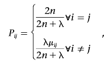where 2n denotes the number of haplotypes for n diploid individuals, λ denotes the normalized mutation rate of l loci (by default, we have λ=2l), and μ_ij denotes the probability of mutating from h_i to h_j according to the number of differing loci between the two haplotypes, conditional on the fact that at least one mutation occurred. When the mutation probability per locus is defined as u and the number of differing loci between h_i and h_j as x, μ_ij can be calculated as

Here, u=1/(2n) indicates one mutation per locus over all n individuals.

Accounting for recombination events

We let θ^(j)_i denote the expected frequency of haplotype h_i after the recombination process is taken into consideration for the first j+1 markers. Then, we have the following recursive relationship:

where θ⁽⁰⁾_i=θ^*_i denotes the frequency of ancestral haplotype h_i=h_i[1,j]∥h_i[j+1,l], and h_i[1,j] and h_i[j+1,l] denote the partial haplotypes of h_i for SNPs 1 to j and for SNPs (j+1) to l, respectively. The final output, f_R(Θ^*)=[θ^(l-1)₁,…,θ^(l-1)_m], gives the expected recombination results on the haplotype frequency. The recombination probabilities (i.e., γ_j values) are related to both the recombination rates and the ages of ancestral haplotypes. We assume, a priori, that γ_j follows an exponential distribution, p(γ_j)∝e^-τγ_j, and infer γ_j from the genotype data G. Here, we set τ=20. A smaller τ encourages more recombination events. We observed that the performance of the algorithm was insensitive to τ∈(10,30).

The joint model

The expected modern-day haplotype frequency f^* needs to incorporate both mutation and recombination processes. We choose f^*=f_R[f_M(Θ^*)] in this study, although other functional forms are also possible.

As mentioned earlier, we assume that α=cf^*, Θ∼Di(Θ|α), and the likelihood function in equation (1) holds. By default, we let c=1 when no genotypes are missing, and we slightly increase c as the amount of missing genotypes increases. A larger value of c implies a higher prior confidence in the coalescence relationship, which can be helpful when there are missing genotypes. We observed that the inference results are not sensitive to the choice of c, as long as it remains small (≪2n). The joint prior distribution of Θ, Θ^*, and γ=(γ₁,…,γ_l-1) can be written as

which leads to the joint distribution of both the parameters and the data

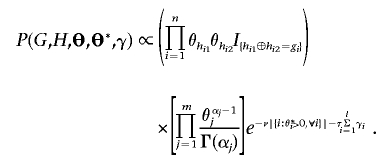Note that, if H is incompatible with G, then P(G,H,Θ,Θ^*,γ)=0. We can further integrate Θ and obtain the marginal posterior distribution of (G_mis,H,Θ^*,γ):

where n_i is the number of copies of haplotype h_i in H and where G_obs and G_mis are the observed and missing genotypes, respectively. By default, we let ν=6. We observed that our method performed suboptimally when ν had small values (e.g., 1 or 2) but was quite robust for larger values of ν.

Given the posterior distribution (2), we can iteratively sample H (and G_mis) and Θ^* by using MCMC and then can infer the most likely haplotype pairs for each individual. In each iteration, our algorithm updates each individual’s haplotype phase conditional on all the other parameters, by sampling from

where H_-i denotes the haplotype phases of all other individuals and n_h is the count of haplotype h in H_-i. This simple structure is similar to that in the work of Niu et al.20 The difference is that the hyperparameter α incorporates a coalescence relationship instead of being completely noninformative. For example, if a haplotype h does not exist in H_-i but is similar to a haplotype in H_-i, then α_h can help increase the chance to sample h. On the other hand, if h is distant from all haplotypes in H_-i, then α_h will be close to 0. Details of the MCMC procedure for updating Θ^* are given in appendix A. If the genotype data are obtained from regions spanning recombination hotspots, our algorithm can also estimate the recombination parameter γ simultaneously. A Langevin-Euler method was employed to update γ more efficiently (appendix A).

Partition Ligation

To handle data with a large number of linked loci, we use the “hierarchical implementation” of the partition-ligation method delineated by Niu et al.20 We first partition all l loci into sequential, contiguous, and nonoverlapping “atomistic units,” such that each atomistic unit consists of ⩽6 loci. Within each unit, haplotypes are sampled from their posterior distributions (note that all model parameters are defined within a unit), as described above. The B most frequently sampled distinct haplotypes are then kept. In the ligation step, we piece together pairs of adjacent units by selecting the top B best candidates among B² possible concatenations of the two adjacent units’ haplotypes. We choose B=m. This strategy drastically reduces the parameter space without a significant loss of information (i.e., low-probability ligation products are tossed away). The inference and ligation steps are repeated until all loci are joined together.

Running-Time Evaluation

Without incorporation of the recombination events, the computation time of our method is O(nl+ml) per iteration, where m is the number of haplotypes, n is the individual sample size, and l is the number of markers. After recombination in the model is considered, the computation time is increased to O(nl+ml²lnl) per iteration because we need to simultaneously update the recombination parameters and compute the recombination effect on haplotype frequencies.

MCMC Convergence Assessment

An important issue in using MCMC for posterior inference is to check the convergence of the algorithm. One approach is to compare samples from several parallel MCMC chains.35 For the CHB algorithm, we performed 2 chains in parallel, starting from different random points. Within the burn-in period, we monitored the ratio of within-chain variations to the overall variation for the log-posterior probability. If multiple chains converge to a common mode (either global or local), the ratio approaches 1. We continued the burn-in period until the ratios for all chains reached a threshold and then started collecting posterior samples. To check the convergence of PHASE under its default settings, we ran PHASE on the HapMap data sets with 10-fold more iterations than its default setting (and hence 10 times the running time). The CHB software package can be obtained from the Coalescence-guided Hierarchical Bayesian Model for Haplotype Inference Web site.

Results

For brevity, we use “CHB-NR” and “PHASE-NR” to denote the application of the “no recombination” modes of CHB and PHASE, respectively, and we use “CHB-R” and “PHASE-R” to denote the application of the “with recombination” modes of CHB and PHASE, respectively.

Coalescence-Based Simulation Data Sets without Recombination

We first ran CHB-NR, PHASE-NR, and HAPLOTYPER on five coalescence-based simulation data sets of sizes n=10, 20, 30, 40, and 50 individuals. Each data set contains 100 independent replicates of genotype data for n individuals, generated by Hudson’s program ms36 (see ms Web site). The mutation rate normalized by the effective population size is 4, and no recombination hotspots are present. This simulation scheme has been used for comparison purposes in several previous studies.20^,22^,29 PHASE-NR was shown to outperform the methods of Xing et al.22 and Kimmel et al.,29 although those two methods also took the coalescence effect into account. We measure the inference accuracy by the average error rate—that is, the total number of incorrectly inferred individuals divided by the total number of individuals with ambiguous solutions. To test the algorithms’ ability to handle missing data, we also produced data sets with 30% of the genotype data removed at random. The results are summarized in figure 2.

Figure 2. .

Mean error rates of CHB-NR (triangles), PHASE-NR (squares), and HAPLOTYPER (diamonds), for coalescence-based simulation data sets with no missing genotypes (left panel) or 30% missing genotypes (right panel).

As expected, both CHB-NR and PHASE-NR outperformed HAPLOTYPER consistently on all the simulated data sets. CHB-NR performed comparably to PHASE-NR in terms of estimation accuracies when no genotypes were missing but outperformed PHASE-NR when 30% of the genotypes were missing (fig. 2). The inference error rates of CHB-NR, PHASE-NR, and HAPLOTYPER were all significantly increased with the presence of missing data. This is likely a result of the fact that the number of compatible haplotype pairs for each individual increases exponentially as the number of heterogeneous or missing genotype increases.

Whitehead Institute’s Inflammatory Bowel Disease (IBD) Data Sets (No Recombination)

We further tested CHB-NR, PHASE-NR, and HAPLOTYPER on empirical data sets generated on the basis of the IBD haplotype block data of Daly et al.37 According to their article, 129 trios were genotyped at 103 loci located on chromosome 5q31, and haplotypes of the 103 loci could be partitioned into 11 blocks in which there exists little recombination. Four SNPs were not included in any of their blocks, probably because those SNPs were located between adjacent blocks. Within each block, we first used PHASE to infer haplotypes of all children in the 129 trios and randomly sampled 40 haplotypes to generate genotypes of 20 individuals. As we did for previous data sets, we also tested the three methods on data sets with 30% missing genotypes. To calculate the average prediction accuracy, we repeated the above procedure 100 times for all blocks. Results for each block and the average error rates are shown in figure 3.

Figure 3. .

Mean error rates and SEs of CHB-NR (white), PHASE-NR (black), and HAPLOTYPER (gray), for Whitehead IBD data sets with no missing genotypes (left panel) or 30% missing genotypes (right panel).

For the Whitehead Institute’s IBD data sets, CHB-NR performed better than PHASE-NR and HAPLOTYPER. PHASE-NR performed worse than HAPLOTYPER when no data were missing but performed better on data sets with missing data. The fact that HAPLOTYPER performed the worst on data sets with missing data may reflect the necessity of the use of coalescence to help infer correct haplotypes when the space of possible solutions is too large.

HapMap Data Sets (No Recombination)

The International HapMap Project,1^,2 genotyped 269 individuals from four ethnic populations—individuals of northern and western European ancestry (CEU), Han Chinese from Beijing, Japanese from Tokyo, and Yoruba from Ibadan, Nigeria (YRI). Haplotype data based on phase I HapMap SNPs on chromosome 10 of these four ethnic groups were obtained. According to the Out-of-Africa hypothesis,38 the European population is likely to have arisen from a population bottleneck hundreds of generations ago,39^–41 and the African population is likely to exhibit the greatest haplotype diversity.40 We chose to focus on the CEU and YRI populations specifically to assess the robustness of CHB-NR, PHASE-NR, and HAPLOTYPER in populations with different evolutionary histories.

For each population, haplotypes were phased from 60 unrelated individuals (120 haplotypes). We randomly selected 100 regions from chromosome 10 with sample sizes of 20, 40, 60, 80, and 100 haplotypes (corresponding to 10, 20, 30, 40, and 50 individuals, respectively). The region-selection criteria were as follows: (i) the region must contain at least six SNPs; (ii) the pairwise D^′ for all pairs of loci within the region must be at least 0.8; (iii) the number of distinct haplotypes within the region must be at least five; and (iv) the most common haplotype within the region must have a frequency of no more than 80%. These criteria were used to avoid the presence of recombination hotspots or overly simplified scenarios for phasing. There were at least 1,600 nonoverlapping regions on chromosome 10 that satisfied the criteria. We further limited the number of SNPs per sample to be at most 30, although all three methods can handle more SNPs.

As shown in figure 4, CHB-NR achieved a better phasing accuracy than did PHASE-NR, on average, and both CHB and PHASE outperformed HAPLOTYPER. Although the evolutionary histories of European and African populations are very different, our method obtained consistent results for both types of data under the same setting. Interestingly, the prediction error rates for the CEU sample were uniformly smaller than those for the YRI sample, probably because of the relatively restricted haplotype diversity in the CEU sample, often attributed to the presence of a population bottleneck (i.e., a smaller pool of founder haplotypes) in the history of western Europeans.

Figure 4. .

Mean error rates and SEs of CHB-NR (white), PHASE-NR (black), and HAPLOTYPER (gray), for HapMap data sets without recombination and with no missing genotypes (left panels) or 30% missing genotypes (right panels). Upper panels, European ancestry. Lower panels, African ancestry.

Data Sets with Recombination Hotspots

To evaluate the performance of CHB-R on data sets with recombination hotspots, we simulated genotype data from regions spanning known recombination hotspots as reported by the International HapMap Project. We simulated data sets with n=10, 20, 30, 40, and 50 CEU and YRI individuals. As demonstrated in figure 5, CHB-R performed uniformly better than CHB-NR and PHASE-NR and performed similar to PHASE-R for CEU data sets. For YRI data sets, however, CHB-R slightly underperformed the other three algorithms (fig. 5). Interestingly, the improvement of PHASE-R over PHASE-NR was also negligible for YRI data sets, indicating that the coalescence model is perhaps not appropriate here because of the great evolutionary complexity in the population of African ancestry. When 30% of genotypes were missing at random, CHB-R consistently outperformed PHASE-R in both CEU and YRI samples. We also tested all methods on data sets with moderate recombination (D′ 0.5–0.9) and obtained similar results (appendix B [online only]).

Figure 5. .

Mean error rates and SEs of CHB-NR (white), CHB-R (light gray), PHASE-NR (black), and PHASE-R (dark gray), for HapMap data sets with recombination hotspots and with no missing genotypes (left panels) or 30% missing genotypes (right panels). Upper panels, European ancestry. Lower panels, African ancestry.

To validate that CHB-R truly captures the recombination effect, we used CHB-R to detect recombination hotspots between physically adjacent SNPs for 1,081 SNPs in a 3-Mb region on chromosome 10 from the HapMap data depository, using recombination hotspots detected by the International HapMap Project as the reference. The recombination parameters were estimated using genotype data of 40 individuals by use of a sliding-window approach with a window size of 12 SNPs, and the sliding window was shifted from left to right by 6 SNPs per sliding step. Recombination probabilities were then estimated by their respective posterior means and then were further averaged across all four different ethnic populations. The top 10% of these probabilities were plotted in the upper panel of figure 6 (the rest of the probabilities were <0.1 and are not shown), which showed a nice match with those reported by the International HapMap Project (lower panel of fig. 6).

Figure 6. .

CHB recombination estimation (upper panel) compared with the HapMap report of recombination rates for 1,081 SNPs across a 3-Mb region (lower panel). The upper panel displays the estimated average recombination probabilities across four populations from the HapMap project. Only values >0.1, which correspond to the highest 10% of recombination probabilities, are shown.

Running-Time Comparison between CHB and PHASE

For data sets consisting of <50 individual genotypes, CHB-NR was ∼2–3 times slower than PHASE-NR, and CHB-R was ∼1–5 times slower than PHASE-R (table 1). The computational burden of CHB arises from the stochastic sampling step of ancestral haplotype parameter Θ^* and the recombination parameter γ (in CHB-R only), which could be mitigated by employing more-efficient sampling schemes. Note that the total number of iterations of an MCMC algorithm ultimately dictates its running time, and the results observed in table 1 were based on the default settings of CHB-NR, CHB-R, PHASE-NR, and PHASE-R.

Table 1. .

Running-Time Comparisons for CHB-NR, PHASE-NR, CHB-R, and PHASE-R with 100 Data Sets^[Note]

	Running Time (min) for Parameter Settings
Method	n=10; l=15±7	n=20; l=17±7	n=30; l=18±6	n=40; l=20±7	n=50; l=20±7
CHB-NR	16.6	25.3	33.3	41.1	46.1
PHASE-NR	5.5	7.9	11.1	17.2	19.2
	n=10;l=13±4	n=20;l=13±4	n=30;l=13±4	n=40;l=12±4	n=50;l=13±4
CHB-R	87.5	99.7	108.2	98.7	126.8
PHASE-R	15.4	35.0	54.4	75.4	121.0

Note.— Running time was measured, with varying numbers of SNPs for different sample sizes (n) and different mean (±SD) numbers of SNPs (l), on a 1.6-GHz PC with 512 MB memory.

PHASE-R estimates recombination parameters from the product of approximate conditionals (PAC) likelihood, which requires many permutations of the observed individuals.25^,42 Larger numbers of permutations are required for larger sample sizes. In comparison, CHB makes direct inferences on the ancestral haplotype frequencies. Hence, its computational time is not as dependent on the sample size as that of PHASE-R. One might expect PHASE-R to run for a longer time than CHB-R when the sample size exceeds a certain threshold. As an example, we tested all methods on five data sets generated by Hudson’s program, consisting of 100, 200, 400, 800, and 1,600 individuals. As shown in table 2, the running time of CHB became shorter than that of PHASE as more individual genotypes needed to be phased. Although still slower than some existing methods, the CHB algorithm (both with and without consideration of recombination) is comparable to PHASE in terms of practicality. All results were measured on a 1.6-GHz personal computer (PC) with 512 MB memory.

Table 2. .

Running-Time Comparisons for CHB-NR, PHASE-NR, CHB-R, and PHASE-R with Five Simulated Data Sets Consisting of n Individuals and l SNPs^[Note]

	Running Time (s) for Parameter Settings
Method	n=100; l=27	n=200; l=24	n=400; l=25	n=800; l=36	n=1,600; l=23
CHB-NR	61	73	114	268	293
PHASE-NR	47	71	139	541	324
CHB-R	265	177	216	492	258
PHASE-R	369	364	381	950	527

Note.— Running time was measured on a 1.6-GHz PC with 512 MB memory.

To check the convergence of PHASE (both PHASE-NR and PHASE-R) under the default settings, we ran PHASE on the HapMap data sets with 10 times more iterations than the default. We did not observe significantly improved phasing accuracy by running longer chains for data sets with no missing data (mostly <0.01 fluctuation around the original accuracy). For CEU data sets with 30% missing genotypes, we observed that the PHASE results were uniformly improved, so that they were almost comparable to those results produced by CHB’s default setting (appendix B [online only]).

Discussion

The present-day carrier haplotypes can be thought of as modified versions of the original ancestral founder haplotypes—modified through historical mutation and recombination events. By taking into account the coalescence process, haplotype phasing algorithms can result in more-accurate results than otherwise.19^,21^,22^,29 The CHB method introduced in this article, although built on the premise of coalescence, does not make any specific assumptions about how evolutionary forces shape the past population demography from generation to generation (fig. 1). Generally speaking, the timescale for the coalescence process is too long (involving too many unobserved intermediary steps) for the ancestral relationship of the modern-day chromosomes to be modeled faithfully.

The CHB method has the desirable property that the influence of the prior distribution of haplotype frequencies, which takes coalescence into consideration, will diminish to zero as the sample size increases. By using both coalescence simulation and empirically derived data sets, which encompass a broad spectrum of scenarios with varying population evolutionary histories, we showed that CHB compares favorably with PHASE and HAPLOTYPER. Furthermore, our data showed that CHB appears to have more advantages in the presence of missing genotypes. Besides the examples shown in the article (with 30% genotypes missing), we also tested CHB and PHASE on data sets with 10% missing genotypes, which is more common in practice, and observed similar results (appendix B [online only]).

CHB-R can provide estimates of recombination probabilities, which is an attractive option by itself. We validated the accuracy of its estimation by using the empirical HapMap data on chromosome 10 (fig. 6). CHB-R can be further improved by incorporation of additional parameters capturing both intermarker distances and background recombination rates.

Differences between CHB and PHASE

The pith of the original PHASE model—a pseudo-Gibbs sampler19^,24—was to encode the coalescence relationship into Gibbs sampling iterations—that is, to update each individual’s phase by sampling from a specially crafted conditional distribution, 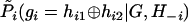. This model was later extended by the inclusion of a recombination parameter and the PAC likelihood42 into MCMC iterations so as to estimate both haplotype frequencies and recombination parameters.25 However, it is still a pseudo-MCMC sampler because the set of conditionals do not correspond to a joint probability distribution.

CHB shares the same coalescence spirit as PHASE, but differs significantly from PHASE in two aspects: (i) CHB uses a hierarchical structure (Θ^*→α→Θ) to directly model the coalescence relationship among modern-day haplotypes, whereas PHASE makes use of the coalescence relationship indirectly through iterative sampling, and (ii) CHB corresponds to a hierarchical Bayesian approach, so that its inference results enjoy the standard analytical support and interpretation common to all Bayesian procedures. In contrast, it is not possible to write down the formal statistical/Bayesian model that underlies PHASE. As a result, the inference results obtained using PHASE (either the new or the old versions) do not have a Bayesian, frequentist, or Fisherian interpretation, although it has been argued that this incoherence does not lead to any practical concerns.24^,25

Differences between CHB and HAPLOTYPER

In HAPLOTYPER, the pseudocount vector α in the prior Dirichlet distribution for haplotype frequencies was made to converge to near zero, so that the prior is nearly noninformative. Although a parsimony solution is favored by this prior distribution, it does not encourage clustering of haplotypes in any way. In contrast, CHB assigns different prior probabilities to different haplotypes according to the ancestral frequency Θ^*, which is inferred jointly with other parameters from the data. CHB also exhibited a significant improvement in performance compared with HAPLOTYPER and PHASE on data sets with a significant amount of missing genotypes, which indicates both the robustness of CHB and a possible disadvantage of using an incoherent inference procedure in PHASE when haplotype phases are more difficult to resolve.

Appendix A

Metropolis-Hastings Recipe for Updating Θ^*

To simplify the computation for updating Θ^*, we first discretize each of its components to be multiples of 1/(2n) and then design a Metropolis-Hastings recipe.43 Two different proposals are implemented. Move 1: randomly select two nontrivial ancestral haplotypes (defined as those with nonzero ancestral frequencies) and then add a small number δ to the frequency of the first haplotype and subtract δ from that of the second one. We let δ equal 1/(2n) by default but can also choose it randomly from 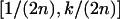, where k is a positive integer. Note that this move may decrease the number of nontrivial haplotypes but can never increase it. Thus, we need move 2: randomly select a trivial haplotype (with zero frequency) and a nontrivial one, change the frequency of the first haplotype to δ, and reduce δ from the frequency of the nontrivial one. This move is necessary to ensure the reversibility. The proposed new is accepted with probability

where π(·) denotes the probability function (1), and T(·,·) is the transition probability. Let the number of nontrivial ancestral haplotypes in state Θ^* be x and let the total number of all possible ancestral haplotypes be m (⩾x); then, we have

where p is the frequency of move 1. The Metropolis-Hastings ratio r is hence calculated correspondingly.

Our conditional probabilities used in the MCMC updates are derived from the joint likelihood function (1). In comparison, the conditional probabilities used in PHASE’s MCMC updates are directly defined as

where

is not derived from a joint prior distribution.19

The Langevin-Euler Move

The Langevin-Euler MCMC update (reviewed by Liu43) uses the information from the derivative of the log-posterior density. It proposes the next move in a sensible direction in the sampling space, such that the proposed move has a reasonable chance to be accepted. In each iteration, we calculate the gradient ∇U=∂U/∂γ, where U=logP(G,H,Θ^*,γ), as in equation (1). We then propose to move γ to 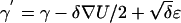and accept the proposal according to the Metropolis-Hastings ratio. Here, δ is a small number controlling the size of each move, and ɛ∼N(0,1).

Appendix B

Running PHASE for Longer Iterations

Figure B1 shows the difference between the phasing accuracy of PHASE running 10 times the number of iterations as the default and the accuracy of PHASE running under the default setting. The only significant improvement was for the CEU data sets with 30% missing genotypes, for which the accuracy was uniformly improved by 1%, on average, for different sample sizes.

Figure B1. .

Difference of phasing accuracy by running PHASE with 10 times number of iterations. M = mutation-only data; M+R = data in which both mutation and recombination are involved; +30% = data sets with 30% missing genotypes. Upper panel, HapMap data sets with European ancestry. Lower panel, HapMap data sets with African ancestry.

CHB and PHASE Results on Data Sets with 10% Missing Genotypes

The figures show the error rate of CHB-NR, PHASE-NR (fig. B2a–B2d), CHB-R, and PHASE-R (fig. B2e and B2f) for various data sets: coalescence-based simulation data sets, Whitehead IBD data sets, CEU data sets from HapMap, and YRI data sets from HapMap. CHB outperformed PHASE in most data sets except YRI data sets with recombination hotspots.

Figure B2. .

Comparison between CHB-NR (triangles) and PHASE-NR (squares) on coalescence-based simulated data set (a), Whitehead IBD data set (b), and two HapMap data sets with no recombination: CEU (c) and YRI (d). In addition, the comparison between CHB-R (triangles) and PHASE-R (squares) of data sets with recombination hotspots is shown for CEU (e) and YRI (f). From each data set, 10% of genotypes were randomly removed.

TAP2 Data Set

This data set from Jeffreys et al.44 contains experimentally determined haplotypes from the TAP2 gene in the major histocompatibility complex region. A total of 45 biallelic markers, including insertion/deletion polymorphisms, were separately typed for 60 individual chromosomes from 30 unrelated United Kingdom whites by use of allele-specific oligonucleotide hybridization. According to Jeffreys et al.,44 there are 28 distinct haplotypes in the sample, and they can be partitioned into three major haplotype blocks. Within each block, we randomly sampled 40 haplotypes to generate genotypes of 20 hypothetical individuals, with and without missing genotypes, and used the three algorithms to infer their haplotypes. The average inference accuracy for each block was calculated using 100 independent samples, and the results are shown in figure B3.

Figure B3. .

Comparison among CHB-NR (white), PHASE-NR (black), and HAPLOTYPER (gray) on TAP2 data sets with no missing genotypes (left panel) or 30% missing genotypes (right panel).

Comparison of Asian Population Data Sets

We compared CHB, PHASE, and HAPLOTYPER for HapMap data sets of Han Chinese and Japanese populations. For each population, data used in figure B4 were generated from regions without recombination hotspots, whereas data used in figure B5 were generated from recombination hotspot regions. HAPLOTYPER does not model recombination events and hence is omitted in figure B5.

Figure B4. .

Comparison between CHB-NR (triangles), PHASE-NR (squares) and HAPLOTYPER (diamonds) on HapMap data sets with no recombinations from different populations: a, Han Chinese population with no missing genotypes; b, Japanese population with no missing genotypes; c, Han Chinese population with 10% missing genotypes; d, Japanese population with 10% missing genotypes; e, Han Chinese population with 30% missing genotypes; f, Japanese population with 30% missing genotypes.

Figure B5. .

Comparison between CHB-NR (white), CHB-R (light gray), PHASE-NR (black) and PHASE-R (dark gray) on HapMap data sets with recombination hotspots from different populations: a, Han Chinese population with no missing genotypes; b, Japanese population with no missing genotypes; c, Han Chinese population with 10% missing genotypes; d, Japanese population with 10% missing genotypes; e, Han Chinese population with 30% missing genotypes; f, Japanese population with 30% missing genotypes.

Comparison of Data Sets with Moderate Recombination

We compared CHB-NR, CHB-R, PHASE-NR, and PHASE-R for additional HapMap data sets of European and African populations. For each population, data used in figure B6 were generated from regions containing moderate recombination with minimum D′ between 0.5 and 0.9.

Figure B6. .

Comparison between CHB-NR (white), CHB-R (light gray), PHASE-NR (black), and PHASE-R (dark gray) on HapMap data sets with moderate recombinations from different populations: a, European population with no missing genotypes; b, African population with no missing genotypes; c, European population with 10% missing genotypes; d, African population with 10% missing genotypes; e, European population with 30% missing genotypes; f, African population with 30% missing genotypes.

References

- 1.International HapMap Consortium (2003) The International HapMap Project. Nature 426:789–796 10.1038/nature02168 [DOI] [PubMed] [Google Scholar]
- 2.International HapMap Consortium (2005) A haplotype map of the human genome. Nature 437:1299–1320 10.1038/nature04226 [DOI] [PMC free article] [PubMed] [Google Scholar]
- 3.Akey J, Jin L, Xiong M (2001) Haplotypes vs single marker linkage disequilibrium tests: what do we gain? Eur J Hum Genet 9:291–300 10.1038/sj.ejhg.5200619 [DOI] [PubMed] [Google Scholar]
- 4.Schaid DJ (2004) Evaluating associations of haplotypes with traits. Genet Epidemiol 27:348–364 10.1002/gepi.20037 [DOI] [PubMed] [Google Scholar]
- 5.Clark AG (2004) The role of haplotypes in candidate gene studies. Genet Epidemiol 27:321–333 10.1002/gepi.20025 [DOI] [PubMed] [Google Scholar]
- 6.Jundson R, Stephens JC (2001) Notes from the SNP vs haplotype front. Pharmacogenomics 2:7–10 10.1517/14622416.2.1.7 [DOI] [PubMed] [Google Scholar]
- 7.Niu T (2004) Algorithms for inferring haplotypes. Genet Epidemiol 27:334–347 10.1002/gepi.20024 [DOI] [PubMed] [Google Scholar]
- 8.Clark AG (1990) Inference of haplotypes from PCR-amplified samples of diploid populations. Mol Biol Evol 7:111–122 [DOI] [PubMed] [Google Scholar]
- 9.Gusfield D (2002) Haplotyping as perfect phylogeny: conceptual frame-work and efficient solutions. In: Proceedings of the 6th Annual International Conference on Computational Biology, Washington, DC, April 18–21. ACM, pp 166–175 [Google Scholar]
- 10.Bafna V, Gusfield D, Lancia G, Yooseph S (2003) Haplotyping as perfect phylogeny: a direct approach. J Comput Biol 10:323–340 10.1089/10665270360688048 [DOI] [PubMed] [Google Scholar]
- 11.Eskin E, Halperin E, Karp RM (2003) Efficient reconstruction of haplotype structure via perfect phylogeny. J Bioinform Comput Biol 1:1–20 10.1142/S0219720003000174 [DOI] [PubMed] [Google Scholar]
- 12.Halperin E, Eskin E (2004) Haplotype reconstruction from genotype data using imperfect phylogen. Bioinformatics 20:1842–1849 10.1093/bioinformatics/bth149 [DOI] [PubMed] [Google Scholar]
- 13.Excoffier L, Slatkin M (1995) Maximum-likelihood estimation of molecular haplotype frequencies in a diploid population. Mol Biol Evol 12:921–927 [DOI] [PubMed] [Google Scholar]
- 14.Hawley ME, Kidd KK (1995) HAPLO: a program using the EM algorithm to estimate the frequencies of multi-site haplotypes. J Hered 86:409–411 [DOI] [PubMed] [Google Scholar]
- 15.Long JC, Williams RC, Urbanek M (1995) An EM algorithm and testing strategy for multiple-locus haplotypes. Am J Hum Genet 56:799–810 [PMC free article] [PubMed] [Google Scholar]
- 16.Chiano MN, Clayton DG (1998) Fine genetic mapping using haplotype analysis and the missing data problem. Ann Hum Genet 62:55–60 10.1017/S0003480098006678 [DOI] [PubMed] [Google Scholar]
- 17.Dempster AP, Laird NM, Rubin DB (1977) Maximum likelihood from incomplete data via EM algorithm. J R Stat Soc Ser B 39:1–38 [Google Scholar]
- 18.Beaumont MA, Rannala B (2004) The Bayesian revolution in genetics. Nat Rev Genet 5:251–261 10.1038/nrg1318 [DOI] [PubMed] [Google Scholar]
- 19.Stephens M, Smith NJ, Donnelly P (2001) A new statistical method for haplotype reconstruction from population data. Am J Hum Genet 68:978–989 [DOI] [PMC free article] [PubMed] [Google Scholar]
- 20.Niu T, Qin ZS, Xu X, Liu JS (2002) Bayesian haplotype inference for multiple linked single-nucleotide polymorphisms. Am J Hum Genet 70:157–169 [DOI] [PMC free article] [PubMed] [Google Scholar]
- 21.Greenspan G, Geiger D (2004) Model-based inference of haplotype block variation. J Comput Biol 11:493–504 10.1089/1066527041410300 [DOI] [PubMed] [Google Scholar]
- 22.Xing E, Sharan R, Jordan MI (2004) Bayesian haplotype inference via the Dirichlet process. In: Proceedings of the Twenty-First International Conference on Machine Learning, Banff, Alberta, July 4–8. ACM, pp 879–886 [Google Scholar]
- 23.Qin ZS, Niu T, Liu JS (2002) Partition-ligation expectation-maximization algorithm for haplotype inference with single-nucleotide polymorphisms. Am J Hum Genet 71:1242–1247 [DOI] [PMC free article] [PubMed] [Google Scholar]
- 24.Stephens M, Donnelly P (2003) A comparison of Bayesian methods for haplotype reconstruction from population genotype data. Am J Hum Genet 73:1162–1169 [DOI] [PMC free article] [PubMed] [Google Scholar]
- 25.Stephens M, Scheet P (2005) Accounting for decay of linkage disequilibrium in haplotype inference and missing-data imputation. Am J Hum Genet 76:449–462 [DOI] [PMC free article] [PubMed] [Google Scholar]
- 26.Marchini J, Cutler D, Patterson N, Stephens M, Eskin E, Halperin E, Lin S, Qin ZS, Munro HM, Abecasis GR, Donnelly P, for the International HapMap Consortium (2006) A comparison of phasing algorithms for trios and unrelated individuals. Am J Hum Genet 78:437–450 [DOI] [PMC free article] [PubMed] [Google Scholar]
- 27.Hudson RR (1983) Properties of a neutral allele model with intragenic recombination. Theor Popul Biol 23:183–201 10.1016/0040-5809(83)90013-8 [DOI] [PubMed] [Google Scholar]
- 28.Hudson RR (1991) Gene genealogies and the coalescent process. In: Futuyma D, Antonovics J (eds) Oxford surveys in evolutionary biology, volume 7. Oxford University Press, Oxford, United Kingdom, pp 1–44 [Google Scholar]
- 29.Kimmel G, Shamir R (2005) GERBIL: genotype resolution and block identification using likelihood. Proc Natl Acad Sci USA 102:158–162 10.1073/pnas.0404730102 [DOI] [PMC free article] [PubMed] [Google Scholar]
- 30.Griffiths RC (1980) Lines of descent in the diffusion approximation of neutral Wright-Fisher models. Theor Popul Biol 17:37–50 10.1016/0040-5809(80)90013-1 [DOI] [PubMed] [Google Scholar]
- 31.Kingman JFC (1982) On the genealogy of large populations. J Appl Prob 19A:27–43 [Google Scholar]
- 32.Kingman JFC (1982) The coalescent. Stochaistic Process Appl 13:235–248 10.1016/0304-4149(82)90011-4 [DOI] [Google Scholar]
- 33.Kingman JFC (1982) Exchangeability and the evolution of large populations. In: Koch G, Spizzichino F (eds) Exchangeability in probability and statistics: proceedings of the International Conference on Exchangeability in Probability and Statistics. North-Holland Publishing, Amsterdam, pp 97–112 [Google Scholar]
- 34.Tajima F (1983) Evolutionary relationship of DNA sequences in finite populations. Genetics 105:437–460 [DOI] [PMC free article] [PubMed] [Google Scholar]
- 35.Gelman A, Rubin DB (1992) Inference from iterative simulation using multiple sequences. Stat Sci 7:457–472 [Google Scholar]
- 36.Hudson RR (2002) Generating samples under a Wright-Fisher neutral model of genetic variation. Bioinformatics 18:337–338 10.1093/bioinformatics/18.2.337 [DOI] [PubMed] [Google Scholar]
- 37.Daly MJ, Rioux JD, Schaffner SF, Hudson TJ, Lander ES (2001) High-resolution haplotype structure in the human genome. Nat Genet 29:229–232 10.1038/ng1001-229 [DOI] [PubMed] [Google Scholar]
- 38.Templeton AR (1997) Out of Africa? What do genes tell us? Curr Opin Genet Dev 7:841–847 10.1016/S0959-437X(97)80049-4 [DOI] [PubMed] [Google Scholar]
- 39.Reich DE, Goldstein DB (1998) Genetic evidence for a Paleolithic human population expansion in Africa. Proc Natl Acad Sci USA 95:8119–8123 10.1073/pnas.95.14.8119 [DOI] [PMC free article] [PubMed] [Google Scholar]
- 40.Ingman M, Kaessmann H, Pääbo S, Gyllensten U (2000) Mitochondrial genome variation and the origin of modern humans. Nature 408:708–713 10.1038/35047064 [DOI] [PubMed] [Google Scholar]
- 41.Reich DE, Cargill M, Bolk S, Ireland J, Sabeti PC, Richter DJ, Lavery T, Kouyoumjian R, Farhadian SF, Ward R, Lander ES (2001) Linkage disequilibrium in the human genome. Nature 411:199–204 10.1038/35075590 [DOI] [PubMed] [Google Scholar]
- 42.Li N, Stephens M (2003) Modelling linkage disequilibrium, and identifying recombination hotspots using SNP data. Genetics 165:2213–2233 [DOI] [PMC free article] [PubMed] [Google Scholar]
- 43.Liu JS (2001) Monte Carlo strategies in scientific computing. Springer-Verlag, New York [Google Scholar]
- 44.Jeffreys AJ, Ritchie A, Neumann R (2000) High resolution analysis of haplotype diversity and meiotic crossover in the human TAP2 recombination hotspot. Hum Mol Genet 9:725–733 10.1093/hmg/9.5.725 [DOI] [PubMed] [Google Scholar]