Farm Scale Evaluations of spring-sown genetically modified herbicide-tolerant crops: a statistical assessment

Abstract

Primary results from the Farm Scale Evaluations (FSEs) of spring-sown genetically modified herbicide-tolerant crops were published in 2003. We provide a statistical assessment of the results for count data, addressing issues of sample size (n), efficiency, power, statistical significance, variability and model selection. Treatment effects were consistent between rare and abundant species. Coefficients of variation averaged 73% but varied widely. High variability in vegetation indicators was usually offset by large n and treatment effects, whilst invertebrate indicators often had smaller n and lower variability; overall, achieved power was broadly consistent across indicators. Inferences about treatment effects were robust to model misspecification, justifying the statistical model adopted. As expected, increases in n would improve detectability of effects whilst, for example, halving n would have resulted in a loss of significant results of about the same order. 40% of the 531 published analyses had greater than 80% power to detect a 1.5-fold effect; reducing n by one-third would most likely halve the number of analyses meeting this criterion. Overall, the data collected vindicated the initial statistical power analysis and the planned replication. The FSEs provide a valuable database of variability and estimates of power under various sample size scenarios to aid planning of more efficient future studies.

1. Introduction

The Farm Scale Evaluations (FSEs) of spring-sown genetically modified herbicide-tolerant (GMHT) crops were conducted in the UK from 2000 to 2002 (Firbank et al. 1999, 2003a,b). The effects of the management regimes associated with conventional and genetically modified beet (Beta vulgaris L.), maize (Zea mays L.) and oilseed rape (Brassica napus L.) crops on weed plant and invertebrate indicators within fields and in field margins were compared. Each crop was treated as a different experiment. The first results were published in October 2003 for vegetation (Heard et al. 2003), soil-surface-active invertebrates (Brooks et al. 2003), epigeal and aerial arthropods (Haughton et al. 2003), field boundary invertebrates and vegetation (Roy et al. 2003), and plant and invertebrate trophic groups (Hawes et al. 2003).

The design considerations and statistical methods developed for the FSEs are described in detail elsewhere (Rothery et al. 2002, 2003; Perry et al. 2003). Briefly, each experiment comprised a randomized block design, with whole fields as blocks and with the treatment (conventional or GMHT) replicated once on half-field units in each field. The primary concerns were with tests of the null hypothesis of no difference in abundance, measured as counts of individuals in each half-field, between the GMHT and conventional treatments, and with estimates of treatment effects.

The FSEs were unusual in at least three ways. First, the FSEs cost £6 m (about £0.5 m crop⁻¹ yr⁻¹), much more than most ecological experiments, corresponding in total to 24 standard research grants (Crawley 2003). Second, they were highly controversial and attracted intense examination because of the public concern over genetic modification (Perry 2003). As a response, the research proposed by the contractors was overseen by a Scientific Steering Committee that scrutinized closely the planned design and analysis which became the subject of considerable discussion and further research (Perry et al. 2003).

Third, Firbank et al. (2003b) and others (Lawton 2003; May 2003; Webb 2003; Pollock 2004) have emphasized the prime importance of the FSE database as a source of baseline measurements of the abundance of biodiversity to inform changes in policy for British agriculture. Research is now showing how biodiversity can be enhanced in arable landscapes by the manipulation of farming systems (Dewar et al. 2003) and their adjacent field margins (Sotherton 1991), and there is a perceived need to restore the balance between agricultural production and wildlife.

For each of the above reasons, it is fair to ask whether the effort that went into planning was justified, whether the original assumptions were vindicated, whether more sites were required or fewer could have been used, whether the analysis of the FSEs was efficient, and how estimates of variability might be used to inform the design of future similar studies. This paper is intended to provide answers to these and similar questions.

2. Background

The statistical power of a significance test is the probability of rejecting the null hypothesis when some given alternative hypothesis is true. Prior to publication of the results, a statistical power analysis (Perry et al. 2003) had suggested that the planned replication of around 60 fields per crop over 3 years would be sufficient to provide useful information from which valid statistical inferences could be drawn. Specifically, it indicated that a sample size of n=60 fields should have provided adequate power (more than 80%) to detect multiplicative differences of R=1.5-fold, for a given biological indicator, so long as its coefficient of variation (CV) did not exceed 50% and its mean abundance exceeded 5.0. Power was estimated over scenarios that encompassed a range of treatment differences, number of fields and degrees of random variability, both for a standard log-Normal model, based on a Normal distribution of logarithmically transformed counts, and also for an extended negative binomial model developed to be more realistic for the count data, particularly for small abundances. For the extended model the variance (V) of the count was assumed to be related to the mean count (μ) through a power law (Taylor 1961) with parameters α and β, i.e. V=αμ^β. The mean count, μ_ij, for treatment i in field j was given by ln μ_ij=γ+F_j+t_i, where γ is the logarithm of the overall mean count (γ=ln[μ], μ=e^γ), F_j is a field effect and t_i is a treatment effect. Note that treatment and field effects were, therefore, multiplicative on the natural count scale (μ_ij=μ exp[F_j]exp[t_i]).

The model was used to simulate count data to estimate power for detecting multiplicative differences R=1.3, 1.5 and 2, using sample sizes n=20, 30, 40, 60 and 90, with mean counts μ=1, 5, 10 and 100, field effects which varied over a 100-fold range, β=1.0, 1.5 and 2, and values of α chosen to achieve coefficients of variation on the natural scale (CV) of 50, 80 and 100%. The power of the Monte Carlo paired randomization test (two-tailed test at the 5% significance level) (Manly 1994) was estimated using 10⁵ sets (500 repetitions of each of 199 randomized sets plus the original data) of simulated data, for each of 12 combinations of the model parameters. Three test-statistics were examined, reflecting three forms of variance–mean relationships defined through β: d, the mean of the differences between the two treatments on a logarithmic scale (β=2); r, the logarithm of the ratio of the overall arithmetic means of the two treatments (β=1); and d_w, a weighted version of d with weights based on the approximate variance of the difference in logarithmically transformed counts, assuming β=1.5.

The analysis reported in the five FSE data papers was a standard randomized block ANOVA. Prior to analysis the total count, c_ij, per half-field for treatment i in field j was transformed to l_ij=log(c_ij+1), after inspection of residuals had suggested that the standard log-Normal model with β=2 provided an adequate model. The realized sample size, n, was the number of fields remaining after excluding those with missing values, and those for which the total whole-field count was zero or one. The null hypothesis was tested with a Monte Carlo paired randomization test using the test-statistic $d={\sum }_j[l_{2j}-l_{1j}]/n$, where n is the number of fields in the analysis, with p-values estimated from 999 random permutations. Treatment effects were estimated by the multiplicative ratio (GMHT/conventional), calculated as R=10^d.

In addition to the published analysis that assumed β=2, two other multiplicative models were fitted which were similar, except they made different assumptions about the relationship between variance and mean expressed through β. One was a standard generalized linear model (GLM; McCullagh & Nelder 1989) with logarithmic link and Poisson error distribution (β=1); the other was a GLM with logarithmic link and power law variance function (β=1.5).

What follows is a statistical assessment of the FSE results for count data for spring-sown crops as published in Heard et al. (2003), Brooks et al. (2003), Haughton et al. (2003), Roy et al. (2003) and Hawes et al. (2003), focusing on estimates of variability and their effect on realized power. Many of the 531 biological indicators tested in those papers were pre-selected on the basis of taxonomic groups, but do not form a random sample because the other criteria for inclusion were mean abundance, and, to a lesser extent, the ecological importance of the test result. Results for other data types (plant biomass, crop canopy, height, etc.) and follow-up samples taken in the two subsequent cropping years are not considered here.

3. Methods

We study the relationships amongst statistical significance, sample size and treatment effect; estimate the actual value of β and various measures of variability; compare the performance of different statistical models for β, and the three test-statistics d, r and d_w; investigate the effects of increasing/reducing the sample size of the FSEs on the realized significance levels; estimate the realized power, and compare it to power estimates for different possible future values of n; and estimate the sample size required to achieve 80 and 90% power in a given percentage of analyses of the measured biological indicators.

(a) Relationships amongst significance level, sample size and treatment effect

A volcano plot (−log(p) versus log(R), Jin et al. 2001) allowed an assessment of the frequency of significant results achieved for various sizes of estimated treatment effect, particularly those greater than 1.5-fold identified by Perry et al. (2003) as effects the FSEs had sought to detect with relatively high frequency. Small values of realized sample size, n, occurred when a biological indicator was relatively rare, so a scatter plot of log(R) versus n allowed an appraisal of whether treatment effects were consistent between abundant and rare species or groups.

(b) Estimation of β

For each of the three fitted multiplicative models described above, the true but unknown value of β was estimated as β_est from the regression coefficient (b) in a linear regression of the logarithm of the absolute standardized residuals on the logarithmically transformed fitted values, i.e. β_est=2b+β (Carroll & Ruppert 1988). A combined estimate β_o was then calculated from the three estimates using linear interpolation to find the value of β for which β_est=β, i.e. the value for which the regression coefficient b in the residual plot is zero (cf Perry 1987).

(c) Summary statistics and measures of variability

Whole-field geometric means, M, measures of variability (CV on natural scale and standard deviation, s, the square-root of the residual mean square of the ANOVA from the published analysis on the natural logarithmic scale) and estimates of β_o were computed for each of 531 reported tests of the null hypothesis for count data. Some summary statistics were tabulated for each of the five indicator groups (FSE papers), for all 531 indicators combined and for each of the three crops. These included: mean, minimum and maximum values of n and CV; median, and lower and upper quartiles of β_o after exclusion of analyses with n<30; and the frequency with which large treatment effects were detected with statistical significance.

(d) Comparison of test-statistics from different models

Since the majority of individual values and all median values of β_o were found to lie between 1.5 and 2, a graphical comparison was made of the 531 published results of tests and estimates of treatment effects using the statistic d (assuming β=2) with the unpublished results based on the statistic r_1.5 (assuming β=1.5).

(e) Significance of d-statistic in relation to sample size

The effect of reducing or increasing the sample size of the FSEs on the realized significance levels was examined. Note that p-values for the Monte Carlo paired randomization test for d were very similar to those for the t-test. This analysis, therefore, uses the p-value for the parametric paired t-test, i.e. t=|d|/s.e.[d], where the standard error of the test-statistic d is based on the residual mean square in the ANOVA for the randomized block design. New t-values, t_n, were calculated for a range of projected sample sizes n_p=kn, where k=0.08, 0.17, 0.33, 0.5, 0.67, 1, 1.5, 2, 3, 6 and 12, using $t_n=t\sqrt{k}$. Corresponding p-values were calculated from Student's t distribution with n_p−1 d.f. The percentage of analyses statistically significant at the 5 and 1% levels were tabulated for each value of k, for each group of indicators and for all 531 indicators combined.

(f) Estimates of statistical power of d-statistic

Statistical power depends upon the chosen experimental design, the magnitude of the effect specified, variability, abundance and replication. For these data, the results of the power analysis (Perry et al. 2003) were used to develop an empirical model to estimate power for detecting a specified difference (R), as follows:

$$\text{Probit}[\text{Power}]=0.955+0.670\theta -0.526\theta /\sqrt{M}-1.46{\beta }_{\text{o}}+0.182\theta {\beta }_{\text{o}}-7.67/\sqrt{n}+3.62{\beta }_{\text{o}}/\sqrt{n},$$

where Probit[] denotes the cumulative distribution of the standardized Normal distribution, the estimated non-centrality parameter, θ, is calculated as $\text{ln}(R)/\sqrt{(2s^2/n)}$, and other terms are as defined earlier (and see the Glossary of statistical terms given in table A1 of the electronic supplementary material). This model has mean absolute error of 1.5 percentage points over the range of power values reported in Perry et al. (2003).

The power of the d-statistic was estimated for each individual indicator with values of treatment effect R=1.1, 1.2, 1.3, 1.4, 1.5 and 2, and for projected sample sizes of n_p=kn, where k=0.08, 0.17, 0.33, 0.5, 1, 1.5, 2, 3, 6 and 12. The numbers of indicators with greater than 80 and 90% power were obtained for each group of indicators and for all 531 indicators combined, for values of R=1.3, 1.5 and 2.

The sample size, n₈₀, required for 80% power was estimated for each indicator for values of R=1.1, 1.2, 1.3, 1.4, 1.5 and 2. Estimates were obtained by solving the equation that defines the non-centrality parameter, θ, iteratively (Conte & De Boor 1980).

Estimates of n₈₀ were adjusted to allow for the difference between the originally planned sample size (n_o) and the realized sample size (n), by multiplying by n_o/n, where n_o=66, 65 and 67 for beet, maize and spring oilseed rape, respectively. Median values and 60-, 70-, 80- and 90-percentiles of the distribution of n₈₀ were calculated for each value of R, for each group of indicators and for all 531 indicators combined.

4. Results

(a) Relationships amongst significance level, sample size and treatment effect

There were 110 indicators in total for which the estimated treatment effect exceeded 1.5-fold (i.e. R>1.5 or R<0.67; shown as symbols outside the two vertical dashed lines in figure 1a), and 82% of these (those above the horizontal line in figure 1a) achieved significance at the 5% level. There was no apparent relationship between the size of the treatment effect and realized sample size, for any of the three crops (figure 1b).

Figure 1.

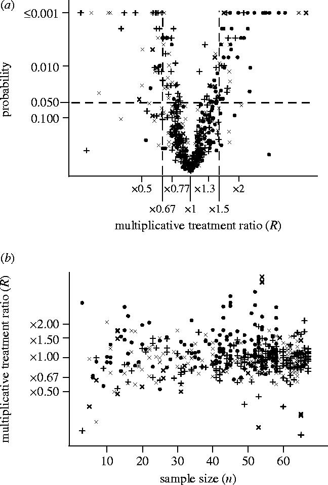
Relationship between significance level, p, from a Monte Carlo paired randomization test, sample size, n, and multiplicative treatment effect, R, for the log-Normal model (β=2), for 531 analyses of count indicators from the primary FSE papers. (a) ‘Volcano’ plot of p, plotted as −log(p), against R, plotted as log R. (b) Scatter plot of R, plotted as log(R), against n. Symbols represent crops: cross-mark, beet; filled-circle, maize; plus, spring oilseed rape.

(b) Summary statistics, estimates of β and measures of variability

Summary statistics for n, CV and β_o are given in table 1. Although individual values varied from less than zero to considerably greater than three, median values of β_o were remarkably consistent between the groups of indicators and the crops, all falling between 1.5 and 2.0, and averaging 1.7 overall. Values of n always exceeded 40 for the vegetation indicators.

Table 1.

Summary statistics for n, CV and β_o, and values of N, N_1.5 and P_1.5. (Values presented for groups of indicators corresponding to primary FSE papers (aerial, Haughton et al. (2003); boundary, Roy et al. (2003); surface, Brooks et al. (2003); trophic, Hawes et al. (2003); vegetation, Heard et al. (2003)) and for all 531 indicators combined (all crops combined in each case), and for each crop (all indicators combined in each case). n is number of fields, and β_o is an estimate of the exponent in the power law relationship between variance and mean abundance, V=αμ^β. The N analyses of count indicators for each group were included in the summaries of n and CV, but only the subset of those analyses with n≥30 were included for β_o. N_1.5 is number of analyses with R>1.5 or R<0.67, and P_1.5 is proportion of those N_1.5 analyses that achieved significance at 5%. Values of n, CV and β_o for all 531 individual analyses are given in table A2 of the electronic supplementary material.)

	group/crop
aerial	boundary	surface	trophic	vegetation	all indicators	beet	maize	spring oilseed rape
N	106	119	151	107	48	531	188	165	178
mean n	40	45	48	51	59	47	47	43	52
min n	3	7	13	6	42	3	5	3	3
max n	65	67	67	67	66	67	66	58	67
mean CV	73.6	72.3	71.0	63.3	96.6	72.6	71.9	75.7	70.4
min CV	9.7	36.1	23.9	16.3	36.7	9.7	9.7	22.0	16.3
max CV	168.4	150.1	193.7	101.9	191.7	193.7	149.1	193.7	150.1
N1.5	19	23	28	13	27	110	37	43	30
P1.5	0.63	0.70	0.93	0.77	0.96	0.82	0.76	0.86	0.83
number of analyses with n≥30	74	90	132	99	48	443	149	134	160
median βo	1.71	1.53	1.67	1.76	1.81	1.68	1.69	1.74	1.61
lower quartile βo	1.38	1.32	1.50	1.49	1.65	1.46	1.43	1.56	1.43
upper quartile βo	2.02	1.75	1.87	1.96	1.97	1.92	1.95	1.96	1.84

Whilst n was very small for some indicators, its mean value usually exceeded 45. Similarly, CV varied from below 10 to almost 200%, but the mean CV was consistent between crops and 73% overall. The mean CV for vegetation indicators, 97%, was notably larger than that for the other indicator groups. This indicates that, although, on average, the power would have been of the order of about 70% to detect an effect of size R=1.5, the actual treatment effect for many indicators was larger than this, especially those for vegetation. Individual values of n, M, CV, β_o and s for each of the 531 indicators are given in table A2 of the electronic supplementary material. Values of s were relatively small for indicators measuring trophic interactions (Hawes et al. 2003) but relatively large for vegetation indicators (Heard et al. 2003).

(c) Comparison of test-statistics from different models

Inferences appeared robust to model misspecification. Values in the scatterplot (figure 2) of treatment effects using test-statistic d (assuming β=2) versus r_1.5 (assuming β=1.5) were clustered tightly around the equality line, especially within the range −0.3<d<0.3, that accounted for over 90% of all values. Only in about 4% of cases would a significant test at the 5% level using one model have given non-significance using the other.

Figure 2.

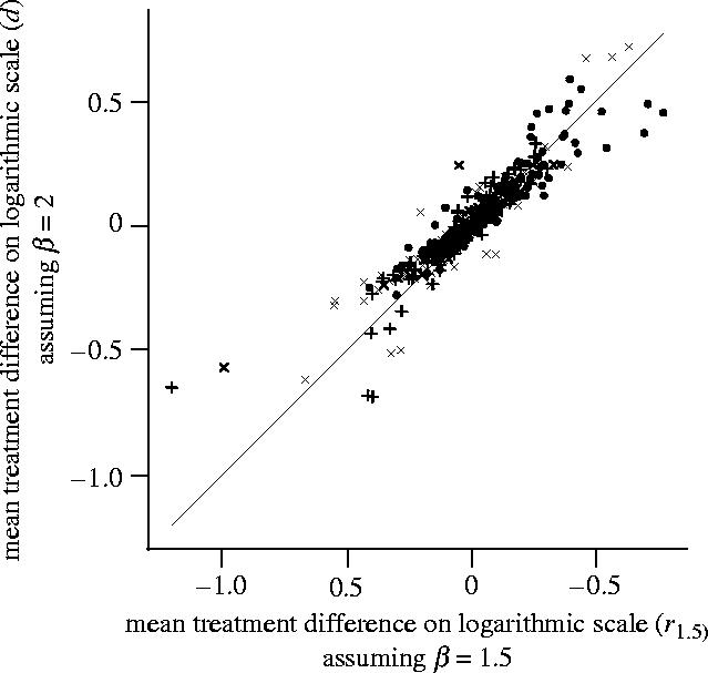
Estimates of treatment effects using the statistics d (assuming β=2) and r_1.5 (assuming β=1.5) for fitted multiplicative models from N=531 analyses of count indicators from the primary FSE papers. Symbols represent crops: cross-mark, beet; filled-circle, maize; plus, spring oilseed rape; and solid line is the equality line where d=r_1.5.

(d) Significance of d-statistic in relation to sample size

The predicted percentage of analyses that would result in a significant treatment difference at 5 and 1%, for various multiples, k, of n, are shown in figure 3 for each of the five groups of indicators and for all 531 indicators combined. Overall achieved percentages, given by k=1, were 27.1% at the 5% level and 15.4% at the 1% level. As expected, projected increases in sample size would improve detectability of effects and vice versa. A halving of sample size would have resulted in a loss of significant results of about the same order. There was a relatively larger number of significant treatment effects for the vegetation indicators reported by Heard et al. (2003). This reflects the fact that herbicide management affects vegetation directly, whereas invertebrates were generally affected less and indirectly (Firbank et al. 2003b).

Figure 3.

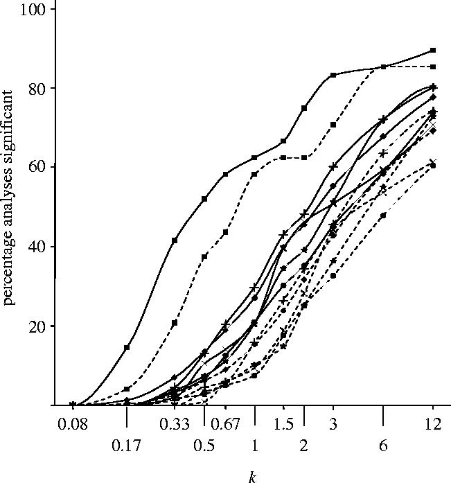
Predicted percentage of analyses that would result in a significant treatment difference at 5% (solid lines) and 1% (dashed lines), for various multiples, k (plotted as log k), of n (number of fields, see table A2 of the electronic supplementary material), for groups of indicators corresponding to primary FSE papers (cross-mark, Haughton et al. 2003; filled-circle, Roy et al. 2003; plus, Brooks et al. 2003; asterisks, Hawes et al. 2003; filled-square, Heard et al. 2003) and for all 531 indicators combined (filled-diamond). Specifically, the achieved percentages (k=1) were, at 5% significance, 20.7, 21.0, 29.8, 20.6 and 62.5 for the five indicator groups and 27.1 for all indicators combined, respectively, and, at 1% significance, 9.4, 7.6, 15.9, 10.3, 58.3 and 15.4, respectively.

(e) Estimates of statistical power of d-statistic

Estimates of the numbers of analyses with greater than 80 and 90% realized power are shown in table 2, for each group of indicators and for all 531 indicators combined. Of course, there is a distribution of power over the different analyses. However, for a particular analysis with a true power value of 80%, we might expect each realization to yield greater than 80% power in approximately half of the cases, which is not greatly dissimilar to the 40% achieved. For values of R≤1.5 a change from ≥80% to the more stringent requirement of ≥90% power reduced the estimated number of analyses achieving this by about one-third, although for R=2 the reduction is not nearly as great. Notably, one in four of the FSE analyses had greater than 90% power to detect an effect of size R=1.5.

Table 2.

Number of analyses (out of N) with ≥80 and 90% estimated realized power, for values of the multiplicative treatment effect R=1.3, 1.5 and 2, for each group of indicators (see table 1) and all 531 indicators combined.

group	N	number of analyses with power ≥80%			number of analyses with power ≥90%
R=1.3	R=1.5	R=2	R=1.3	R=1.5	R=2
aerial	106	3	21	69	1	13	51
boundary	119	9	47	73	2	28	67
surface	151	28	68	120	22	48	111
trophic	107	25	58	94	16	43	89
vegetation	48	4	17	38	2	15	33
all indicators	531	69	211	394	43	147	351

The extent to which the percentage of analyses with power greater than 80% is increased by projected increases of sample size and reduced by decreases is quantified in figure 4. Note that a reduction in sample size of just one-third, here represented by a decrease from about n=67 to n=44, would likely almost halve the number of analyses meeting this criterion. Results for the case of greater than 90% power are in table A3 of the electronic supplementary material.

Figure 4.

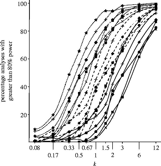
Percentage of analyses with ≥80% power for various multiples, k (plotted as log k), of n (number of fields, see table A2 of the electronic supplementary material), and three values of the multiplicative treatment effect, R=1.3 (solid line), 1.5 (dashed line) and 2 (dotted line), for groups of indicators corresponding to primary FSE papers and for all 531 indicators combined (symbols as in figure 3). The number of analyses with ≥90% power is given in table A3 of the electronic supplementary material. Values for the observed sample (k=1) are summarized for both thresholds in table 2 of this paper.

Median values of the sample size, n₈₀, required for 80% power are shown in table 3. Values of n lie, as expected, between the tabulated values for R=1.5 and R=2. If greater certainty of large power is required then sample sizes must be increased; estimated sample sizes required to achieve at least 80% power in 60, 70, 80 and 90% of analyses are presented in figure A1 of the electronic supplementary material.

Table 3.

Median value of estimated sample size, n₈₀, required for 80% power, for values of the multiplicative treatment effect R=1.1, 1.2, 1.3, 1.4, 1.5 and 2. (Median values are given for each group of indicators (see table 1) and all 531 indicators combined, are each computed over N analyses (see table 1), and represent the initial sample size (number of fields) required to achieve 80% power in 50% of analyses. Estimated sample sizes required to achieve at least 80% power in 60, 70, 80 and 90% of analyses are presented in figure A1 of the electronic supplementary material.)

group	R=1.1	R=1.2	R=1.3	R=1.4	R=1.5	R=2
aerial	1936	551	283	181	127	51
boundary	1487	412	204	128	90	34
surface	1119	330	169	106	76	28
trophic	931	263	130	80	57	21
vegetation	1399	399	200	125	89	33
all indicators	1327	370	185	116	82	31

5. Discussion

Prior to the FSEs, there was very sparse data on measures of variability for any biological indicators at the scale of plot size of half- or whole-fields; hence the ability to predict power was restricted (Perry et al. 2003). The results did confirm the choice of the range of variability in counts used in the power analysis and the percentage of tests that achieved statistical significance slightly exceeded 80%. Although there was no guarantee that this would be the case in 1999 at the planning stage, interim unpublished analyses during 2000 and 2001 for a limited number of sites gave confidence that this would be the case. Had this not been true, sample sizes could have been increased in the later years of the FSEs; Firbank et al. (2003b) emphasized that treatment effects were consistent with no evidence of interactions of treatment with years.

The lack of a relationship between the size of the treatment effect and realized sample size gives confidence that effects are consistent between rare and abundant species. This is important, since many species of conservation value in arable ecosystems may suffer effects such as a ‘double jeopardy’ from being rare and restricted in range (Lawton 1993); monitoring of their biodiversity requires special care.

The statistical model adopted for the FSE data was justified. Results from Clark et al. (1996) and earlier authors indicated that values of β should be, on average, less than 2 but somewhat greater than 1.5, as used in the power analysis (Perry et al. 2003). Whilst the estimated average value for β was, at 1.7, closer to 1.5 than to 2, the value assumed by the published analyses, there would have been very little difference in the inferences drawn had β been assumed to be 1.5.

Vegetation in the FSEs probably provided the most important biological indicators, being affected by direct herbicidal effects (Firbank et al. 2003b). Vegetation indicators were generally surprisingly variable, as measured by CV and s. However, sample size for vegetation indicators was generally large and n always exceeded 40. Also, treatment effect size was usually large; 22 of the 48 analyses had values of R>2. These large values of n and R more than offset the large variability, and explained the large realized power for vegetation indicators. By contrast, low abundance resulted in some very small values of n for analyses in the aerial paper; this frequently prevented the epigeal invertebrate indicators concerned from being analysed with great power.

In summary, for such a costly experiment it was proper to make a considerable initial effort to plan and to estimate the replication required to achieve the desired power. This analysis has shown this effort to have been entirely justified, and vindicated the original assumptions. It suggests that any future projects of major ecological importance or risk assessments of important novel agricultural practices may merit similar inputs. It reflects a growing trend in recent years to give greater prominence to power calculations. These have often been hampered by lack of knowledge concerning variability, but this was not the case here.

New EU legislation, both for genetically modified crops and non-genetically modified applications, requires the effects of various agricultural practices on biodiversity to be studied as part of the regulatory and registration processes, and monitored subsequently. The FSEs provide a valuable database of variability (see statistics given in table A2 of the electronic supplementary material) that enables future such studies to be planned more efficiently than could have been the case previously. The more direct comparisons of estimated power under various scenarios of sample size, presented here, will assist predictions of power and significance levels for future studies, similar to the FSEs, which for reasons of cost may not be as well resourced.

References

- Brooks D.R, et al. Invertebrate responses to the management of genetically modified herbicide-tolerant and conventional spring crops. I. Soil-surface-active invertebrates. Phil. Trans. R. Soc. B. 2003;358:1847–1862. doi: 10.1098/rstb.2003.1407. 10.1098/rstb.2003.1407 [DOI] [PMC free article] [PubMed] [Google Scholar]
- Carroll R.J, Ruppert D. Chapman & Hall; New York: 1988. Transformation and weighting in regression. [Google Scholar]
- Clark S.J, Perry J.N, Marshall E.J.P. Estimating Taylor's power law for weed species and the effect of spatial scale. Weed Res. 1996;36:405–417. [Google Scholar]
- Conte S.D, de Boor C. 3rd edn. McGraw-Hill; New York: 1980. Elementary numerical analysis: an algorithmic approach. [Google Scholar]
- Crawley M.J. 2003. Chairman's introduction to the FSE results presentation, 16 October 2003.https://www.rothamstead.bbsrc.ac.uk/pie/sadie/reprints/RI_Introduction.ppt [Google Scholar]
- Dewar A.M, May M.J, Woiwod I.P, Haylock L.A, Champion G.T, Garner B.H, Sands R.J, Qi A, Pidgeon J.D. A novel approach to the use of genetically modified herbicide tolerant crops for environmental benefit. Proc. R. Soc. B. 2003;270:335–340. doi: 10.1098/rspb.2002.2248. 10.1098/rspb.2002.2248 [DOI] [PMC free article] [PubMed] [Google Scholar]
- Firbank L.G, Dewar A.M, Hill M.O, May M.J, Perry J.N, Rothery P, Squire G.R, Woiwod I.P. Farm-scale evaluation of GM crops explained. Nature. 1999;399:727–728. 10.1038/21516 [Google Scholar]
- Firbank L.G, et al. An introduction to the Farm-Scale Evaluations of genetically modified herbicide-tolerant crops. J. Appl. Ecol. 2003a;40:2–16. 10.1046/j.1365-2664.2003.00787.x [Google Scholar]
- Firbank L.G, et al. 2003b. The implications of spring-sown genetically modified herbicide-tolerant crops for farmland biodiversity: a commentary on the Farm Scale Evaluations of spring sown crops.http://www.defra.gov.uk/environment/gm/fse/results/fse-commentary.pdf [Google Scholar]
- Haughton A.J, et al. Invertebrate responses to the management of genetically modified herbicide-tolerant and conventional spring crops. II. Within-field epigeal and aerial arthropods. Phil. Trans. R. Soc. B. 2003;358:1863–1877. doi: 10.1098/rstb.2003.1408. 10.1098/rstb.2003.1408 [DOI] [PMC free article] [PubMed] [Google Scholar]
- Hawes C, et al. Responses of plants and invertebrate trophic groups to contrasting herbicide regimes in the Farm Scale Evaluations of genetically modified herbicide-tolerant crops. Phil. Trans. R. Soc. B. 2003;358:1899–1913. doi: 10.1098/rstb.2003.1406. 10.1098/rstb.2003.1406 [DOI] [PMC free article] [PubMed] [Google Scholar]
- Heard M.S, et al. Weeds in fields with contrasting conventional and genetically modified herbicide-tolerant crops. I. Effects on abundance and diversity. Phil. Trans. R. Soc. B. 2003;358:1819–1832. doi: 10.1098/rstb.2003.1402. 10.1098/rstb.2003.1402 [DOI] [PMC free article] [PubMed] [Google Scholar]
- Jin W, Riley R.M, Wolfinger R.D, White K.P, Passador-Gurgel G, Gibson G. The contributions of sex, genotype and age to transcriptional variance in Drosophila melanogaster. Nat. Genet. 2001;29:389–395. doi: 10.1038/ng766. 10.1038/ng766 [DOI] [PubMed] [Google Scholar]
- Lawton J.H. Range, population abundance and conservation. Trends Ecol. Evol. 1993;8:409–413. doi: 10.1016/0169-5347(93)90043-O. 10.1016/0169-5347(93)90043-O [DOI] [PubMed] [Google Scholar]
- Lawton J.H. The Guardian. 2003 17 October 2003. [Google Scholar]
- Manly B.F.J. 2nd edn. Chapman & Hall; London: 1994. Randomization, bootstrap and Monte Carlo methods in biology. [Google Scholar]
- May R.M. 2003. Royal Society submission to ACRE consultation on GM farm-scale evaluations.http://www.royalsoc.ac.uk/document.asp?id=1358 [Google Scholar]
- McCullagh P, Nelder J.A. 2nd edn. Chapman & Hall; London: 1989. Generalized linear models. [Google Scholar]
- Perry J.N. Iterative improvement of a power transformation to stabilise variance. Appl. Stat. 1987;36:15–21. [Google Scholar]
- Perry J.N. Genetically-modified crops. Sci. Christ. Belief. 2003;15:141–163. [Google Scholar]
- Perry J.N, Rothery P, Clark S.J, Heard M.S, Hawes C. Design, analysis and statistical power of the Farm Scale Evaluations of genetically modified herbicide-tolerant crops. J. Appl. Ecol. 2003;40:17–31. 10.1046/j.1365-2664.2003.00786.x [Google Scholar]
- Pollock C.J. Why it's time for GM Britain. The Guardian. 2004 26 February 2004. [Google Scholar]
- Rothery P, Clark S.J, Perry J.N. Proc. Invited Pap. XXI Int. Biometric Soc. Con., Freiburg, Germany, July 2002. 2002. Design and analysis of Farm-Scale Evaluations of genetically modified herbicide-tolerant crops. [Google Scholar]
- Rothery P, Clark S.J, Perry J.N. Design of the farm-scale evaluations of genetically modified herbicide-tolerant crops. Environmetrics. 2003;14:711–717. 10.1002/env.619 [Google Scholar]
- Roy D.B, et al. Invertebrates and vegetation of field margins adjacent to crops subject to contrasting herbicide regimes in the Farm Scale Evaluations of genetically modified herbicide-tolerant crops. Phil. Trans. R. Soc. B. 2003;358:1879–1898. doi: 10.1098/rstb.2003.1404. 10.1098/rstb.2003.1404 [DOI] [PMC free article] [PubMed] [Google Scholar]
- Sotherton N.W. Conservation headlands: a practical combination of intensive cereal farming and conservation. In: Firbank L.G, Carter N, Darbyshire J.F, Potts G.R, editors. The ecology of temperate cereal fields. Blackwell Scientific Publications; Oxford: 1991. pp. 373–397. [Google Scholar]
- Taylor L.R. Aggregation, variance and the mean. Nature. 1961;189:732–735. [Google Scholar]
- Webb J. Editorial: a victory for reason. New Sci. 2003;180 No. 2418, 25 October 2003. [Google Scholar]
Associated Data
This section collects any data citations, data availability statements, or supplementary materials included in this article.