Adherence to antiretroviral HIV drugs: how many doses can you miss before resistance emerges?

Abstract

The question of determining how many doses may be skipped before HIV treatment response is adversely affected by the emergence of drug-resistance is addressed. Impulsive differential equations are used to develop a prescription to minimize the emergence of drug-resistance for protease-sparing regimens. A threshold for the maximal number of missable doses is determined. If the number of missed doses is below this threshold, then resistance levels are negligible and dissipate quickly, assuming perfect adherence subsequently. If the number of missed doses exceeds this threshold, even for 24 h, resistance levels are extremely high and will not dissipate for weeks, even assuming perfect adherence subsequently. After this interruption, the minimum number of successive doses that should be taken is determined. Estimates are provided for all protease-sparing drugs approved by the US Food and Drug Administration. Estimates for the basic reproductive ratios for the wild-type and mutant strains of the virus are also calculated, for a long-term average fractional degree of adherence. There are regions within this fraction of adherence where the outcome is not predictable and may depend on a patient's entire history of drug-taking.

1. Introduction

Advances in HIV therapeutics have changed the nature of the disease, so that it has now assumed some of the characteristics of a chronic disease (Friedland & Williams 1999). Although the use of highly active antiretroviral therapy in the treatment of HIV infection has led to considerable improvement in morbidity and mortality, without strict patient adherence to complex drug regimens, viral replication may ensue and drug-resistant strains of the virus may emerge (Altice & Friedland 1998). Adherence levels greater than 95% are required to maintain virologic suppression, but actual adherence rates are often far lower; most studies show that 40–60% of patients are less than 90% adherent and adherence also tends to decrease over time (Bartlett 2002). It is necessary to understand the degree of medication adherence needed to effectively and durably control HIV replication; or, conversely, how many doses of medication can be missed before treatment response is adversely affected (Tennenberg 1999).

Adherence to HIV therapy presents special issues that result from the biology of HIV, the magnitude of the required therapeutic effort, and the changing demography of HIV infection (Altice & Friedland 1998). Potent and continuous suppressive therapy for the duration of viral replicative capability is necessary for therapy to be effective (Friedland & Williams 1999). Recent data indicate that each antiretroviral therapeutic class has a unique adherence–resistance relationship (Bangsberg et al. 2004). Protease inhibitor (PI)-sparing regimens have been shown to have equivalent potency to PI-containing regimens (Staszewski et al. 1999), are suitable for once-daily dosing (Gatell 1998) and may reduce the risk of metabolic and potential cardiovascular consequences of therapy relative to some PI-based regimens, while providing similar or improved virologic control and durability of effect (Moyle 2003). Resistance to non-nucleoside reverse transcriptase inhibitor therapy occurs at low to moderate levels of adherence (Bangsberg et al. 2004).

A handful of mathematical models have attempted to quantify the degree of adherence (Wahl & Nowak 2000; Philips et al. 2001; Tchetgen et al. 2001; Huang et al. 2003, 2004; Ferguson et al. 2005). A recent overview of mathematical models for adherence, as well as structured treatment interruptions (STIs), can be found in Heffernan & Wahl (2005a). The use of impulsive differential equations to model dynamic drug concentrations during HIV-1 therapy has recently been proposed (Smith & Wahl 2004). This framework facilitated an investigation of drug classes with different mechanisms of action. In Smith & Wahl (2005), this approach was extended to examine the conditions required for the emergence of drug-resistance during HIV therapy, for PI-sparing regimens, assuming perfect adherence.

In this paper, the effects of individual drugs in PI-sparing regimens are considered. Two strains of the virus are assumed: a wild-type (drug sensitive) strain that initially dominates and a mutant (drug-resistant) strain, which has lower infectivity. As in Smith & Wahl (2005), drugs levels are divided into three regions. Low drug levels will not affect either strain, intermediate drug levels will affect the wild-type strain of the virus alone, and high drug levels will affect both strains. The aim of this study is to answer the following questions. (i) How many doses can a strongly adherent patient miss before drug-resistance emerges? (ii) How many successive doses should be subsequently taken after this ‘drug holiday’ to return to strong adherence? Furthermore, a method to elucidate the basic reproductive ratio, based on the overall pattern of adherence, is provided, extending the work of Wahl & Nowak (2000) to impulsive differential equations. This includes an example to illustrate the effects that the pattern of adherence may have and shows that, under certain circumstances, a patient's entire history of adherence may be critical.

2. Modelling adherence

The dynamics of drugs can be split into three regions: in region 1, drug levels are insufficient to inhibit viral replication in either the wild-type or mutant strain of the virus. In region 2, drug levels are sufficient to inhibit viral replication in the wild-type strain, but not the mutant strain. In region 3, drug levels are sufficiently high to inhibit viral replication in both strains of the virus. The dynamics of the wild-type and mutant virions, the various classes of T cells and the PI-sparing drugs can be modelled using a system of impulsive differential equations (see appendix A). An impulse may or may not occur, depending whether the drug is taken or not. If a dose occurs at prescribed time t_k, the impulse effect applies; if a dose does not occur, no dose is taken until at least time t_k+1, at which point the same decision of whether or not a dose is to be taken is applied.

Impulsive differential equations consist of a system of ordinary differential equations (ODEs), together with difference equations. Between ‘impulses’ t_k the system is continuous, behaving as a system of ODEs. At the impulse points, there is an instantaneous change in state in some or all of the variables. This instantaneous change can occur when certain spatial, temporal or spatio-temporal conditions are met. The interested reader is referred to Bainov & Simeonov (1989, 1993, 1995) and Lakshmikantham et al. (1989) for more details on the theory of impulsive differential equations.

(a) Minimizing drug-resistance

Let R₁ denote the threshold drug value between regions 1 and 2 and R₂ denote the threshold drug value between regions 2 and 3. That is, if R<R₁, then the drug levels cannot inhibit either strain, if R₁<R<R₂, then the drug will inhibit the wild-type strain but not the mutant, and if R>R₂, then the drug will inhibit both strains of the virus. Clearly, the most desirable case is R>R₂, so that the drug is controlling both the wild-type and the mutant. The threshold R₂ will vary, depending on the degree of resistance the mutant exhibits. Figure 1 demonstrates two possibilities for the drug Abacavir: 10- and 50-fold resistance. For 10-fold resistance R₂=e⁻⁶, whereas for 50-fold resistance R₂=e⁻⁴. For both mutations, R₁=e⁻⁸.

Figure 1.

Example dose–effect curves for the wild-type (solid curve), 10-fold resistant (dashed curve) and 50-fold resistant (dot–dashed curve) viral strains. Note that the x-axis is on a logarithmic scale. When drug concentration R is less than R₁ (region 1), the probability that a T cell absorbs sufficient drug to block infection is negligible for all strains. Between thresholds $R_1<R<R_2^{(10)}$ (region 2), only the wild-type strain has a non-negligible probability of being blocked by the drug. For $R>R_2^{(10)}$ (region 3) both the wild-type and 10-fold resistant strains have non-negligible probability of being blocked by the drug (the dose–effect curves in these regimes are much closer to linear than suggested by this semi-log plot). The threshold $R_2^{(50)}$ represents the equivalent threshold for the 50-fold resistant viral strain. IC₅₀ values for Abacavir were used in this example.

Initally, suppose the patient is adhering to therapy and the drug levels are sufficient to control both strains of the virus, assuming perfect adherence. As successive doses are missed, the drug levels will fall until they reach region 2. At this point there are two options: (i) if therapy is resumed, then drug levels will increase and any emergent mutant strain will be controlled; see figure 2a. (ii) If more doses are missed, then resistance will emerge, since the drug is no longer capable of controlling the mutant strain of the virus; see figure 2b. Figure 2 shows the viral load for the wild-type and 50-fold resistant strains to Didanosine. To prevent the emergence of drug-resistance, drug levels should remain in region 3. See appendix A for details.

Figure 2.

Viral load and drug levels for therapy interruption. Therapy was allowed to reach the impulsive periodic orbit before being interrupted. Data used is for the drug Didanosine. (a, top) Viral load for the wild-type (solid line) and the mutant (dashed line) strains. (b, top) Drug levels on a log scale. (a) Eleven doses were missed, allowing drug levels to enter region 2 briefly before subsequent doses were taken. In this case, the emergence of the mutant strain is negligible and diminishes quickly. (b) Thirteen doses were missed, allowing drug levels to remain in region 2 for 24 h before subsequent doses were taken. In this case, the resistant strain reach almost 60 000 μmol l⁻¹ and was not eliminated for some weeks. Data used were n_I=262.5 day⁻¹, ω=0.7, r_I=0.01 day⁻¹, r_Y=0.005 day⁻¹, d_V=3 day⁻¹, d_S=0.1 day⁻¹, d_I=0.5 day⁻¹, r_P=r_R=r_Q=80 μM⁻¹ day⁻¹, λ=180 cells μl⁻¹ day⁻¹, m_RI=m_RY=log(2) day⁻¹, in addition to data found in table 1.

In figure 2a, 11 doses were missed, while in figure 2b, 13 doses were missed. Didanosine is taken twice a day, so the drug levels remained in region 2 for approximately 24 h, resulting in a spike in resistance levels of the order of 10⁴ μM. Note that with perfect adherence subsequently, drug levels returned to pre-interruption levels within a week, but the resistant strain took approximately 35 days to be eliminated. For patients who miss doses but whose drug levels do not enter region 2, it was also possible to determine the number of doses which should subsequently be taken in order to return to pre-interruption levels. See appendix A.

To illustrate, eight nucleoside reverse transcriptase inhibitors, three non-nucleoside reverse transcriptase inhibitors and a fusion inhibitor were simulated. The threshold values R₁ and R₂ for each drug were determined by using the appropriate IC₅₀ values, in a manner similar to that of figure 1. In each case, the resistant mutant was assumed to confer 50-fold resistance to the drug. The number of missable doses was calculated (see appendix A), as well as the number of successive doses that should be taken subsequently. The results are summarized in table 1.

Table 1.

Summary of data and results for nucleoside, nucleotide and non-nucleoside reverse transcriptase inhibitors and fusion inhibitor. (The intracellular half-life was used when it was known, since nucleoside intracellular half-lives differ greatly from the half-life in plasma. The decay rate d_R was calculated according to the formula d_R=24 log(2)/T_1/2, where T_1/2 is the half-life. The threshold levels for 10- and 50-fold resistance (R₂⁽¹⁰⁾ and R₂⁽⁵⁰⁾, respectively) were calculated using an antiviral effect limit of 1×10⁻³ (see figure 1). The penultimate column shows the number of doses that may be missed before 50-fold resistance emerges, assuming that the drug is able to control the mutant strain with perfect adherence. The final column shows the number of successive doses that must be taken after missing these doses, to be within a 1% tolerance of perfect adherence. In all cases, the numbers of missable and subsequent doses were estimated conservatively; for example, the missable dose threshold for Emtricitabine was 16.49 doses, while the subsequent dose threshold was 10.79, so this translates to 16 missable doses and 11 subsequent doses.)

drug	Ri (μM)	τ (days)	T1/2 (h)	R1 (μM)	$R_2^{(10)}$ (μM)	$R_2^{(50)}$ (μM)	missable	subsequent
Abacavir (ABC)	12	1/2	15	e−8	e−6	e−4	13	9
Didanosine (ddI)	4.65	1/2	25	e−5	e−3	e−1	11	14
Emtricitabine (FTC)	7.2	1	39	e−8	e−6	e−4	16	11
Lamivudine (3TC)	6	1/2	17	e−5	e−2	e−1	7	10
Stavudine (d4T)	2.144	1/2	7	e−6	e−4	e−2	2	4
Tenofivir (TDF)	1.184	1	17	e−5	e−3	e−2	1	4
Zalcitabine (ddC)	0.1008	1/3	3	e−8	e−6	e−4	1	1
Zidovudine (ZDV)	4.24	1/3	3	e−12	e−10	e−8	5	3
Delavirdine (DLV)	35	1/3	5.8	e−7	e−5	e−3	7	5
Efavirenz (EFV)	12.9	1	45	e−8	e−6	e−4	20	13
Nevirapine (NVP)	7.5	1/2	35	e−10	e−7	e−6	40	20
Enfuvirtide (T20)	18.36	1/2	3.8	e−9	e−7	e−5	3	3

(b) Multiple resistance and combination therapy

A drug may have multiple resistant strains which will move the location of R₂. In this case, clearly the highest of all possible R₂ values (see figure 1) should be used to determine the appropriate number of missable doses. For example, if a patient has both 10- and 50-fold viral resistance to Stavudine, then the value $R_2^{(50)}={\text{e}}^{-2}$ should be used to determine the number of missable doses, rather than $R_2^{(10)}={\text{e}}^{-4}$.

Combination therapy of more than one drug will also result in different R₁ and R₂ values for each drug. In this case, there are two approaches. First is to determine the number of missable doses for each drug used in combination and apply the smallest number to the combination as a whole. For example, the combination drug Trizivir consists of Abacavir (6.5 days of missable doses for 50-fold resistance), Lamivudine (3.5 days of missable doses) and Zidovudine (1.67 days of missable doses), so Trizivir would have up to 1.67 days of missable doses before therapy should be interrupted, assuming 50-fold resistance.

Conversely, a patient taking the same combination of Abacavir, Lamivudine and Zidovudine as separate pills per day, would simply apply the results independently. Thus, the patient could miss up to 13 doses of Abacavir, but only five doses of Zidovudine. It should be noted that these recommendations each assume that the dose–effect curves for each drug are not altered by the presence of other drugs in the combination. While this is unlikely to be the case, it can nevertheless be argued that the estimates provided here are conservative, since the probability of the resistant mutation emerging under combination therapy is significantly smaller than the probabilities of emergence for each drug.

The second approach is to apply the results concurrently. For the combination mentioned above, resistance would emerge to Zidovudine after 1.67 days (five doses), effectively reducing the triple-drug combination to dual therapy after that time. After a further 3.5 days (seven doses), resistance to Lamivudine could emerge, making the combination effectively a single-drug combination. Finally, after a further 6.5 days (13 doses), resistance to Abacavir emerges and therapy has failed. This would suggest a window of 11.67 days for this combination.

In Ananworanich et al. (2003), one patient (Patient 41503) taking Zidovudine–Lamivudine–Abacavir, undergoing an STI of one week on/one week off, had developed significant mutations by week 4 (corresponding to two weeks free of therapy, though not concurrently). Another (Patient 99950), taking Zidovudine–Lamivudine–Efavirenz, developed mutation by week 8 (corresponding to a total of four weeks of therapy interruption). A third (Patient 25180), taking Zidovudine–Lamivudine–Nevirapine, did not develop mutations until week 36 (18 total weeks of therapy interruption). The timeframe is not precise, because it discounts any time-delay from combination therapy, as well as the stifling effect on resistance that resumption of therapy during these weeks will have. However, it is broadly consistent with the results presented here.

3. Patterns of adherence

Many patients are known to be only partially adherent. Thus, the results of Wahl & Nowak (2000) on fractional degrees of adherence are extended to impulsive differential equations. The inhibition of viral replication s can be described by

$$s(t)=\frac{{\text{IC}}_{50}}{R(t)+{\text{IC}}_{50}},$$ 3.1

where IC₅₀ is the concentration of drug which inhibits viral replication by 50%. Hence, when s≈1 the drug has no effect, while if s≈0 the drug completely inhibits viral replication. Although, the relationship between in vitro susceptibility of HIV to antiviral drugs and the in vivo inhibition of viral replication in humans has not been rigorously established, the in vitro IC₅₀ values for each drug are used to provide an estimate of the in vivo value of s. The mean value of s, $\overline{s}(p)$, will be calculated, where p is the fraction of adherence. That is, p is the long-term average number of doses that are actually taken divided by the number of prescribed doses; when p=0, set $\overline{s}=1$.

For imperfect adherence, $\overline{s}(p)$ will depend on the patient's entire history of adherence, which is unlikely to be known. In appendix B, a formula for $\overline{s}(p)$ is calculated using this history, but estimates are also provided that are independent of the history of drug taking.

The basic reproductive ratio R₀ for each strain of the virus can be calculated. R₀ is defined as the average number of secondary infected cells arising from one infected cell placed into an entirely susceptible cell population. See Heffernan et al. (2005) for a recent overview. The mean values of the basic reproductive ratios are:

$$R_0^{(\text{I})}(p)=\frac{{{\displaystyle \overline{s}}}_{\text{I}}(p)r_{\text{I}}\lambda }{d_{\text{S}}{d}_{\text{I}}}\text{and}{R}_0^{(\text{Y})}(p)=\frac{{\overline{s}}_{\text{Y}}(p)r_{\text{Y}}\lambda }{d_{\text{S}}{d}_{\text{I}}}.$$

These results mirror those of Wahl & Nowak (2000); while the concentration of drugs is explicit in the model from Smith & Wahl (2005), r_I and r_Y are equivalent to β₁ and β₂, respectively, in Wahl & Nowak (2000), since they are the (constant) rates of infection when drugs are not present. The key difference here is that each ${{\displaystyle \overline{s}}}_i(p)$ can be estimated using two curves, based on the minimum and maximum estimates.

The mean values of these reproductive ratios serve as useful predictors of the long-term outcome of the system under several conditions: (i) the chance extinction of the drug-resistant strain is unlikely (true for HIV); (ii) the time-scale of consistent dose taking or doses missed is short compared to the characteristic times; and (iii) the variations in $R_0^{(\text{I})}$ and $R_0^{(\text{Y})}$ are relatively smooth (this is true, for example, when doses decay smoothly and the dose–response curve is described by equation (3.1)). It should be noted, however, that the long-term averages of $R_0^{(I)}$ and $R_0^{(Y)}$ are not simple functions of p, but also depend on the pattern of dose taking.

To illustrate, suppose that the probability of taking a dose at the beginning of each interval is independent of previous history and is constant. Then, for each new dosing interval, the drug is taken with a probability equal to the long-term average adherence p. This is a Poisson model of adherence, with the probability that i successive doses were missed after the last dose was taken given by $P_i(p)=p{(1-p)}^i$.

Figure 3 shows the regions of dominance for each strain of the virus, using the Poisson model and the estimates derived in appendix B. The wild-type strain (within the solid curves) is assumed to be dominant, in the absence of drugs. The mutant strain (within the dashed curves) is less susceptible to the drugs. The upper and lower curves are derived from the extreme cases of either: (i) perfect adherence or (ii) no prior history of drug-taking (see appendix B). The p-axis can be subdivided into various segments.

1. For $0\le p<{\alpha }_1$, the wild-type strain dominates.

2. For ${\alpha }_1<p<{\beta }_2$, the outcome depends on the dosing pattern or the history of adherence; in this case, either the wild-type or mutant strain could dominate.

3. For ${\beta }_2<p<{\mu }_1$, the mutant strain dominates, while the wild-type is driven to extinction.

4. For ${\mu }_1<p<{\mu }_2$, the outcome depends on the dosing pattern or the history of adherence; in this case either the mutant strain dominates or both strains of the virus are eliminated.

5. For ${\mu }_2<p\le 1$, both strains of the virus are eliminated.

Figure 3.

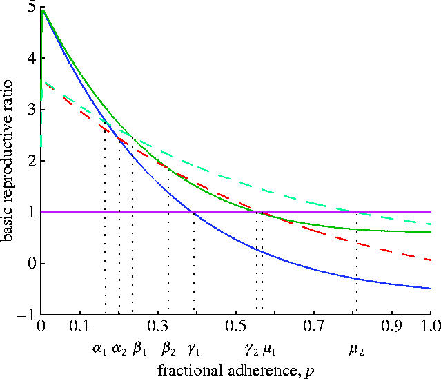
Upper and lower bounds for each strain of the virus. In the absence of drugs (p=0), the wild-type virus dominates. As the fraction of adherence increases, the mutant may dominate. For a sufficiently high fraction, both strains have a basic reproductive ratio of less than 1 and hence the virus is controlled. However, there are regions where the upper and lower bounds of one strain interfere with the bounds of the other strain. In these cases, it is not possible to predict which strain will dominate and the outcome will depend on the patient's entire history of drug-taking.

The critical regions are ${\alpha }_1<p<{\beta }_2$ and ${\mu }_1<p<{\mu }_2$. In these regions, the history of adherence will play a crucial role in determining the outcome.

Figure 4 illustrates two examples, using parameters drawn from the region ${\alpha }_1<p<{\beta }_2$ with a 25.5% fraction of adherence. In figure 4a, the wild-type strain dominates, while in figure 4b the mutant strain dominates. Both figures use identical parameters and the same program was run; only the random seed determining whether a dose is taken or not was different. This parameter was represented by a random variable, drawn from a uniform distribution, scaled to reflect the degree of adherence p.

Figure 4.

The sensitivity of results to the history of drug-taking. The solid lines represent T cells infected with the wild-type strain of the virus and the dashed lines represent T cells infected with the mutant strain. (a) In this case the wild-type strain dominates. Data used was n_I=262.5, ω=0.8, r_I=0.02, r_Y=0.01, d_V=3, d_S=0.1, d_I=0.5, r_R=40, r_Q=10.4, d_R=log(2)/2, λ=180, m_RI=24 log(2)/8, m_RY=24 log(2)/8, R₁=3, R₂=6, IC₅₀ (wild-type)=0.053, IC₅₀ (mutant)=0.53, β_T=0.0014, β_Y=0.001, τ=4, Rⁱ=4, p=0.255. (b) The same data was used and the same program run. However, in this case, the mutant strain dominates. The difference in results is due to the history of drug taking, modelled as a random variable drawn from a uniform distribution. Small changes in the random variable can have a dramatic impact on the outcome.

4. Discussion

A patient who is usually strongly adherent may miss an acceptable number of doses before resistance emerges, without paying an undue cost. Subsequently, the patient must take a certain number of doses in succession, but this number is not too high before drug levels return to pre-interruption levels. However, if more doses are missed before therapy resumes, the cost is unacceptably high. Even if the mutant strain is allowed to emerge for 24 h for Didanosine, the viral load may reach 60 000 μmol l⁻¹ before therapy returns to pre-interruption levels. Furthermore, the length of time that the patient must remain perfectly adherent is extremely long. Thus, a small ‘drug holiday’ may be acceptable, but the length of acceptable holidays will vary with each drug, as will the number of subsequent doses that must be taken in succession.

The number of missable doses varies from no more than 1 (Zalcitabine; thus patients may skip this drug for no more than 16 h, although drug levels will be back to 99% of pre-interruption levels after a single dose) to 40 (Nevirapine; corresponding to a drug holiday of 20 days, but subsequently perfect adherence is required for 10 days in order to achieve 99% of pre-interruption levels), assuming 50-fold resistance. While the actual numbers are illustrative, the method presented here (identify the region 2 threshold, R₂, for the resistant strain in question; calculate the number of missable and subsequent doses using appendix A) is a general method for any PI-sparing drug. This method provides clarity for patients who may plan drug holidays, for those who have inadvertently begun such a holiday or for physicians prescribing temporary relief from drug-related side-effects.

It is important to note that these results assume that the drug is initially controlling both the wild-type and mutant strains and those patients are usually strongly adherent. This also assumes that the threshold values are small compared to the magnitude of a single dose, but this is the case for all PI-sparing drugs currently available (see table 1). Furthermore, the use of impulsive differential equations assumes that the drugs take effect immediately. While some drugs have a short time-to-peak (e.g. Didanosine), others do not. Nevertheless, HIV models using impulsive differential equations have matched results from non-impulsive models with significant accuracy (Huang et al. 2004; Heffernan & Wahl 2005b). It is also assumed that a dose is either taken, or not, precisely at the prescribed times, ignoring the potential behaviour that non-adherent patients may exhibit, such as taking a dose later than prescribed, or taking twice the doses at the next prescription time. The emergence of drug-resistance also depends on treatment experience and other host factors, which are ignored here. Nevertheless, the method presented here is potentially applicable to any future PI-sparing drug, whose mechanism of protection acts to prevent the virus from transcribing its RNA into host DNA.

For patients who are not strongly adherent, the second part of this paper assumes that patients have a long-term average fractional degree of adherence p. The effect of this fraction is shown in figure 3, using estimates for parameters that would otherwise rely on the entire history of a patient's drug-taking. The outcome is not always predictable, depending on which region the fraction of adherence is in.

For a Poisson model of adherence, with fractional adherence taken from one of these key regions, it can be shown that the outcome does indeed change, depending on the patient's drug-taking history. In figure 4, the same fraction of adherence was used and the same program run, yet the long-term results differ in each case. This difference is due to the random seed the program uses to determine whether a dose was taken or not, scaled to the same fraction of adherence. For example, two patients with 50% adherence may have very different results if the first patient takes 50 doses and then skips 50 doses, while the second patient takes every other dose. It should also be noted that small fluctuations could lead to the re-emergence of a strain, even if that strain is close to zero. Thus, the concept of ‘winning’ the competition may not be so clear-cut.

Future work will involve the development of a model to account for the inclusion of PIs, in order to determine the effect that adherence to protease-including regimens may have, as well as a method to quantify how many doses must be taken if drug levels do enter region 2. Further investigation of complicating effects added by combination therapy is also warranted.

Appendix A

Appendix A. The number of missable and subsequent doses

The mathematical model, from Smith & Wahl (2005), is

$$\frac{\text{d}{V}_{\text{I}}}{\text{d}t}=n_{\text{I}}\omega T_{\text{I}}-d_{\text{V}}{V}_{\text{I}}-r_{\text{I}}{T}_{\text{S}}{V}_{\text{I}},$$

$$\frac{\text{d}{V}_{\text{Y}}}{\text{d}t}=n_{\text{I}}\omega T_{\text{Y}}-d_{\text{V}}{V}_{\text{Y}}-r_{\text{Y}}{T}_{\text{S}}{V}_{\text{Y}}-r_{\text{Y}}{T}_{\text{RI}}{V}_{\text{Y}},$$

$$\frac{\text{d}{V}_{\text{NI}}}{\text{d}t}=n_{\text{I}}(1-\omega )(T_{\text{I}}+T_{\text{Y}})-d_{\text{V}}{V}_{\text{NI}},$$

$$\frac{\text{d}{T}_{\text{S}}}{\text{d}t}=\lambda -r_{\text{I}}{T}_{\text{S}}{V}_{\text{I}}-r_{\text{Y}}{T}_{\text{S}}{V}_{\text{Y}}-d_{\text{S}}{T}_{\text{S}}-\theta r_{\text{P}}{r}_{\text{R}}{T}_{\text{S}}R+m_{\text{RI}}{T}_{\text{RI}},$$

$$\frac{\text{d}{T}_{\text{I}}}{\text{d}t}=r_{\text{I}}{T}_{\text{S}}{V}_{\text{I}}-d_{\text{I}}{T}_{\text{I}},$$

$$\frac{\text{d}{T}_{\text{Y}}}{\text{d}t}=r_{\text{Y}}{T}_{\text{S}}{V}_{\text{Y}}-d_{\text{I}}{T}_{\text{Y}}+r_{\text{Y}}{T}_{\text{RI}}{V}_{\text{Y}},$$

$$\frac{\text{d}{T}_{\text{RI}}}{\text{d}t}=\theta r_{\text{P}}{r}_{\text{R}}{T}_{\text{S}}R-r_{\text{Y}}{T}_{\text{RI}}{V}_{\text{Y}}-(d_{\text{S}}+m_{\text{RI}})T_{\text{RI}}+m_{\text{RY}}{T}_{\text{RY}}-\eta r_{\text{Q}}{T}_{\text{RI}}R,$$

$$\frac{\text{d}{T}_{\text{RY}}}{\text{d}t}=\eta r_{\text{Q}}{T}_{\text{RI}}R-(d_{\text{S}}+m_{\text{RY}})T_{\text{RY}},$$

for t≠t_k, where

$$\theta =\{\begin{array}{ll}0,\hfill & \text{if}R<R_1,\hfill \\ 1/r_{\text{R}},\hfill & \text{if}{R}_1<R<R_2,\hfill \\ 1/r_{\text{P}},\hfill & \text{if}R>R_{2,}\hfill \end{array}$$

$$\eta =\{\begin{array}{cc}0,& \text{if}R<R_2,\\ 1,& \text{if}R>R_2.\end{array}$$

Here, V_I and V_Y denote infectious wild-type and mutant virus, respectively, V_NI denotes non-infectious virus, T_S denotes the population of susceptible (non-infected) CD4⁺T cells, T_I denotes the population of CD4⁺T cells infected with the wild-type virus, T_Y denotes the cells infected with the mutant virus, T_RI denotes non-infected cells which have absorbed sufficient quantities of the drug so that the wild-type strain is inhibited, but not enough to prevent infection by the mutant strain of the virus, T_RY denotes non-infected cells which have absorbed sufficient quantities of the drug so that both strains of the virus are inhibited, t is time in days, n_I is the number of virions produced per infected cell per day, ω is the fraction of virions produced by an infected T cell which are infectious, d_V is the rate at which free virus is cleared, d_S is the non-infected CD4⁺T cell death rate, d_I is the infected CD4⁺T cell death rate, r_I is the rate at which wild-type virus infects T cells, r_Y is the rate at which the drug-resistant virus infects T cells, r_P is the rate at which the drug inhibits the wild-type T cells when drug concentrations are in region 2, r_R and r_Q are the rates at which the drug inhibits the wild-type and drug-resistant T cells, respectively, when drug concentrations are in region 3. The constant λ represents a source of susceptible cells, while m_RI and m_RY are the rates at which the drug is cleared from the intracellular compartment for intermediate and high drug concentrations, respectively.

The dynamics of the drug are

$$\frac{\text{d}R}{\text{d}t}=-d_{\text{R}}R,t\ne t_k,$$

with impulse conditions, at times t=t_k:

$$\mathrm{\Delta }R=\{\begin{array}{ll}{R}^i,\hfill & \text{if}\text{a}\text{dose}\text{is}\text{to}\text{be}\text{taken},\hfill \\ 0,\hfill & \text{if}\text{no}\text{dose}\text{is}\text{to}\text{be}\text{taken}.\hfill \end{array}$$

Here, d_R is the rate at which the drug is cleared and Rⁱ is the dosage. Note that, by the definition of an impulsive effect, assuming a dose was taken at time t_k:

$$R(t_k^{+})=R(t_k^{-})+R^i.$$

From Smith & Wahl (2005), for perfect adherence, there is an impulsive periodic orbit in the drug levels, with endpoints

$$\frac{R^i}{1-{\text{e}}^{-d_{\text{R}}\tau }}\text{and}\frac{R^i{\text{e}}^{-d_{\text{R}}\tau }}{1-{\text{e}}^{-d_{\text{R}}\tau }}.$$

For realistic drugs and dosing schedules, $R_2-R_1\ll R^i$ and $((R^i{\text{e}}^{-d_{\text{R}}\tau })/(1-{\text{e}}^{-d_{\text{R}}\tau }))\gg R_2$. (Note that there is a scaling error on the x-axis of figure 1b in Smith & Wahl (2005).) That is, with perfect adherence, drug levels will be comfortably within region 3 and if drug levels fall into regions 1 or 2, a single dose is sufficient to return to region 3. See figure 2.

Thus, assuming perfect adherence, after the nth dose, drug levels satisfy:

$$R(t_n^{+})=\frac{R^i}{1-{\text{e}}^{-d_{\text{R}}\tau }}.$$

If h doses are subsequently missed, then

$$R(t_{n+h}^{-})=\frac{R^i{\text{e}}^{-h{d}_{\text{R}}\tau }}{1-{\text{e}}^{-d_{\text{R}}\tau }}.$$

The condition required to avoid region 2 is $R(t_{n+h}^{-})>R_2$. Hence

$$\frac{R^i{\text{e}}^{-h{d}_{\text{R}}\tau }}{1-{\text{e}}^{-d_{\text{R}}\tau }}>R_2,$$

$$h<\frac{1}{d_{\text{R}}\tau }\text{log}\frac{R^i}{R_2(1-{\text{e}}^{-d_{\text{R}}\tau })}.$$ A1

Thus, if h doses are missed, as long as condition (A 1) is satisfied, drug levels will not reach region 2.

Subsequently, suppose k doses are taken in succession. In order to return to drug levels approximating pre-interruption values, we require

$$R(t_{n+h+k}^{-})>\frac{R^i{\text{e}}^{-d_{\text{R}}\tau }}{1-{\text{e}}^{-d_{\text{R}}\tau }}-ϵ,$$

for some required level of tolerance ϵ. Using impulsive theory:

$$\begin{array}{c}R(t_{n+h}^{+})=R^i+\frac{R^i{\text{e}}^{-h{d}_{\text{R}}\tau }}{1-{\text{e}}^{-d_{\text{R}}\tau }},\\ R(t_{n+h+1}^{-})=R^i{\text{e}}^{-d_{\text{R}}\tau }\left(1+\frac{{\text{e}}^{-h{d}_{\text{R}}\tau }}{1-{\text{e}}^{-d_{\text{R}}\tau }}\right),\\ R(t_{n+h+1}^{+})=R^i\left(1+{\text{e}}^{-d_{\text{R}}\tau }+\frac{{\text{e}}^{-(h+1)d_{\text{R}}\tau }}{1-{\text{e}}^{-d_{\text{R}}\tau }}\right),\\ R(t_{n+h+2}^{-})=R^i{\text{e}}^{-d_{\text{R}}\tau }\left(1+{\text{e}}^{-d_{\text{R}}\tau }+\frac{{\text{e}}^{-(h+1)d_{\text{R}}\tau }}{1-{\text{e}}^{-d_{\text{R}}\tau }}\right),\\ ⋮\\ \begin{array}{l}R(t_{n+h+k}^{-})=R^i{\text{e}}^{-d_{\text{R}}\tau }\left(1+{\text{e}}^{-d_{\text{R}}\tau }+\cdots +{\text{e}}^{-(k-1)d_{\text{R}}\tau }+\frac{{\text{e}}^{-(h+k-1)d_{\text{R}}\tau }}{1-{\text{e}}^{-d_{\text{R}}\tau }}\right)\\ =R^i{\text{e}}^{-d_{\text{R}}\tau }\left(\frac{1-{\text{e}}^{-k{d}_{\text{R}}\tau }}{1-{\text{e}}^{-d_{\text{R}}\tau }}+\frac{{\text{e}}^{-(h+k-1)d_{\text{R}}\tau }}{1-{\text{e}}^{-d_{\text{R}}\tau }}\right).\end{array}\end{array}$$

Hence

$$\begin{array}{cc}R(t_{n+h+k}^{-})-\frac{R^i{\text{e}}^{-d_{\text{R}}\tau }}{1-{\text{e}}^{-d_{\text{R}}\tau }}=& \frac{R^i{\text{e}}^{-(k+1)d_{\text{R}}\tau }({\text{e}}^{-(h-1)d_{\text{R}}\tau }-1)}{1-{\text{e}}^{-d_{\text{R}}\tau }}>-ϵ\\ & \frac{R^i{\text{e}}^{-(k+1)d_{\text{R}}\tau }(1-{\text{e}}^{-(h-1)d_{\text{R}}\tau })}{1-{\text{e}}^{-d_{\text{R}}\tau }}<ϵ.\end{array}$$

Thus, the required number of doses to return to within ϵ of perfect adherence satisfies:

$$k>\frac{1}{d_{\text{R}}\tau }\text{log}\left[\frac{R^i(1-{\text{e}}^{-(h-1)d_{\text{R}}\tau })}{ϵ(1-{\text{e}}^{-d_{\text{R}}\tau })}\right]-1.$$

Appendix B

Appendix B. Mean value of the inhibitory effect $\overline{s}(p)$

For perfect adherence, $\overline{s}$ is just the area under s(t) for one dosing interval, divided by the length of the interval τ. From Smith & Wahl (2005):

$$\begin{array}{r}\hfill R(t)=\frac{R^i{\text{e}}^{-d_{\text{R}}t}}{1-{\text{e}}^{-d_{\text{R}}\tau }}=R(t_k^{+}){\text{e}}^{-d_{\text{R}}t},t_k\le t<t_{k+1}\end{array}.$$

Thus

$$\overline{s}(p)=\frac{1}{\tau }{\int }_0^{\tau }s(t)\text{d}t=\frac{{\text{IC}}_{50}}{\tau }{\int }_0^{\tau }\frac{1}{R(t_k^{+}){\text{e}}^{-d_{\text{R}}t}+{\text{IC}}_{50}}\text{d}t=\frac{1}{d_{\text{R}}\tau }\text{log}{{\displaystyle \left[\frac{R(t_k^{+}){\text{e}}^{-d_{\text{R}}t}+{\text{IC}}_{50}}{R(t_k^{+}){\text{e}}^{-d_{\text{R}}t}}\right]}}_0^{\tau }=\frac{1}{d_{\text{R}}\tau }\text{log}\left[\frac{R(t_k^{+})+{\text{IC}}_{50}{\text{e}}^{d_{\text{R}}\tau }}{R(t_k^{+})+{\text{IC}}_{50}}\right]=\frac{1}{d_{\text{R}}\tau }\text{log}\left[\frac{R^i+{\text{IC}}_{50}({\text{e}}^{d_{\text{R}}\tau }-1)}{R^i+{\text{IC}}_{50}(1-{\text{e}}^{-d_{\text{R}}\tau })}\right].$$

For imperfect adherence, it is assumed that a single dose was taken at time zero. If n−1 doses have been missed and a dose is taken at time t_k, then

$$R^i<R(t_k^{+})\le \frac{R^i}{1-{\text{e}}^{-d_{\text{R}}\tau }}.$$ B1

The left-hand inequality comes from assuming that the drug levels were zero immediately before the dose at time t_k. It should be noted that since a dose was taken at time zero, the true minimum possible is actually $R^i{\text{e}}^{-d_{\text{R}}{t}_k}$; however, for simplicity it can be assumed that this may be arbitrarily close to zero (if t_k is large), which explains the strict inequality. The right-hand inequality comes from assuming perfect adherence until t_k.

The mean $\overline{s}(p)$ can be computed as a weighted average of the areas under s(t) after a dose is taken, after a single dose is missed, after two successive doses are missed, etc. Suppose a dose was taken at time t_k. Let $A_i^{(k)}$ be the area under s(t) for a dosing interval that occurs immediately after i doses have been missed in succession. Then

$$A_i^{(k)}={\int }_{i\tau }^{(i+1)\tau }\frac{{\text{IC}}_{50}}{R(t_k^{+}){\text{e}}^{-d_{\text{R}}t}+{\text{IC}}_{50}}\text{d}t=\frac{1}{d_{\text{R}}}\text{log}{{\displaystyle \left[\frac{R(t_k^{+}){\text{e}}^{-d_{\text{R}}t}+{\text{IC}}_{50}}{R(t_k^{+}){\text{e}}^{-d_{\text{R}}t}}\right]}}_{i\tau }^{(i+1)\tau }=\frac{1}{d_{\text{R}}}\text{log}\left[\frac{R(t_k^{+}){\text{e}}^{-d_{\text{R}}\tau i}+{\text{IC}}_{50}{\text{e}}^{d_{\text{R}}\tau }}{R(t_k^{+}){\text{e}}^{-d_{\text{R}}\tau i}+{\text{IC}}_{50}}\right].$$ B2

Computing (B 2) requires knowing $R(t_k^{+})$, which depends on the patient's history of adherence. However, this is highly unlikely to be known. Using (B 1), $A_i^{(k)}$ can be approximated by

$$A_{i,\text{min}}<A_i^{(k)}<A_{i,\text{max}},$$

where

$$\begin{array}{c}{A}_{i,\text{min}}=\frac{1}{d_{\text{R}}}\text{log}\left[\frac{R^i({\text{e}}^{-d_{\text{R}}\tau i}-{\text{e}}^{-d_{\text{R}}\tau (i+1)})+{\text{IC}}_{50}({\text{e}}^{d_{\text{R}}\tau }-1)}{R^i{\text{e}}^{-d_{\text{R}}\tau i}+{\text{IC}}_{50}(1-{\text{e}}^{-d_{\text{R}}\tau })}\right],\\ A_{i,\text{max}}=\frac{1}{d_{\text{R}}}\text{log}\left[\frac{R^i{\text{e}}^{-d_{\text{R}}\tau i}+{\text{IC}}_{50}({\text{e}}^{d_{\text{R}}\tau }-1)}{R^i({\text{e}}^{-d_{\text{R}}\tau i}-{\text{e}}^{-d_{\text{R}}\tau (i+1)})+{\text{IC}}_{50}(1-{\text{e}}^{-d_{\text{R}}\tau })}\right].\end{array}$$

The estimates A_i,min and A_i,max are independent of the history of drug taking.

Let P_i(p) be the probability that i successive doses were missed after the last dose was taken. In particular, P_i(p) depends on the pattern of adherence, whereas $R(t_k^{+})$ depends on the patient's history of drug taking. It follows that:

$$\overline{s}(p)=\sum _{i=0}^{\infty }\frac{P_i(p)A_i^{(k)}}{\tau }.$$

References

- Altice F.L, Friedland G.H. The era of adherence to HIV therapy. Ann. Intern. Med. 1998;129:503–505. doi: 10.7326/0003-4819-129-6-199809150-00015. [DOI] [PubMed] [Google Scholar]
- Ananworanich J, et al. Failures of 1 week on, 1 week off antiretroviral therapies in a randomized trial. AIDS. 2003;17:F33–F37. doi: 10.1097/00002030-200310170-00001. doi:10.1097/00002030-200310170-00001 [DOI] [PubMed] [Google Scholar]
- Bainov D.D, Simeonov P.S. Ellis Horwood Ltd; Chichester, UK: 1989. Systems with impulsive effect. Stability, theory and applications. [Google Scholar]
- Bainov D.D, Simeonov P.S. Longman Scientific and Technical; Burnt Mill: 1993. Impulsive differential equations: periodic solutions and applications. [Google Scholar]
- Bainov D.D, Simeonov P.S. World Scientific; Singapore: 1995. Impulsive differential equations: asymptotic properties of the solutions. [Google Scholar]
- Bangsberg D.R, Moss A.R, Deeks S.G. Paradoxes of adherence and drug resistance to HIV antiretroviral therapy. J. Antimicrob. Chemother. 2004;53:696–699. doi: 10.1093/jac/dkh162. doi:10.1093/jac/dkh162 [DOI] [PubMed] [Google Scholar]
- Bartlett J.A. Addressing the challenges of adherence. J. Acq. Immun. Def. Synd. 2002;29(Suppl. 1):2–10. doi: 10.1097/00126334-200202011-00002. [DOI] [PubMed] [Google Scholar]
- Ferguson N.M, Donnelly C.A, Hooper J, Ghani A.C, Fraser C, Bartley L.M. Adherence to antiretroviral therapy and its impact on clinical outcome in HIV-infected patients. J. R. Soc. Interface. 2005;2:349–363. doi: 10.1098/rsif.2005.0037. doi:10.1098/rsif.2005.0037 [DOI] [PMC free article] [PubMed] [Google Scholar]
- Friedland G.H, Williams A. Attaining higher goals in HIV treatment: the central importance of adherence. AIDS. 1999;13(Suppl.1):61–72. [PubMed] [Google Scholar]
- Gatell J.M. Early antiretroviral therapy: rationale, protease inhibitor-sparing regimens and once daily dosing. Antivir. Ther. 1998;3(Suppl. 4):49–53. [PubMed] [Google Scholar]
- Heffernan J.M, Wahl L.M. Treatment interruptions and resistance: a review. In: Tan W.-Y, Wu H, editors. Deterministic and stochastic models for AIDS epidemics and HIV infection with interventions. World Scientific; Hackensack, NJ: 2005a. pp. 425–455. [Google Scholar]
- Heffernan J.M, Wahl L.M. Monte Carlo estimates of natural variation in HIV infection. J. Theor. Biol. 2005b;236:137–153. doi: 10.1016/j.jtbi.2005.03.002. doi:10.1016/j.jtbi.2005.03.002 [DOI] [PubMed] [Google Scholar]
- Heffernan J.M, Smith R.J, Wahl L.M. Perspectives on the basic reproductive ratio. J. R. Soc. Interface. 2005;2:281–293. doi: 10.1098/rsif.2005.0042. doi:10.1098/rsif.2005.0042 [DOI] [PMC free article] [PubMed] [Google Scholar]
- Huang Y, Rosenkranz S, Wu H. Modeling HIV dynamics and antiviral response with consideration of time-varying drug exposures, adherence and phenotypic senstitivity. Math. Biosci. 2003;184:165–186. doi: 10.1016/s0025-5564(03)00058-0. doi:10.1016/S0025-5564(03)00058-0 [DOI] [PubMed] [Google Scholar]
- Huang, Y., Liu, D. & Wu, H. 2004 Hierarchical Bayesian methods for estimation of parameters in a longitudinal HIV dynamic system. See http://www.urmc.rochester.edu/smd/biostat/people/faculty/manuscripts/bayesian_yh_jul04.pdf (Accessed September 23 2005.) [DOI] [PMC free article] [PubMed]
- Lakshmikantham V, Bainov D.D, Simeonov P.S. World Scientific; Singapore: 1989. Theory of impulsive differential equations. [Google Scholar]
- Moyle G. Protease inhibitor-sparing regimens: new evidence strengthens position. J. Acq. Immun. Def. Synd. 2003;33(Suppl. 1):17–25. [PubMed] [Google Scholar]
- Philips A.N, Youle M, Johnson M, Loveday C. Use of a stochastic model to develop understanding of the impact of different patterns of antiretroviral drug use on resistance development. AIDS. 2001;15:2211–2220. doi: 10.1097/00002030-200111230-00001. doi:10.1097/00002030-200111230-00001 [DOI] [PubMed] [Google Scholar]
- Smith R.J, Wahl L.M. Distinct effects of protease and reverse transcriptase inhibition in an immunological model of HIV-1 infection with impulsive drug effects. Bull. Math. Biol. 2004;66:1259–1283. doi: 10.1016/j.bulm.2003.12.004. doi:10.1016/j.bulm.2003.12.004 [DOI] [PubMed] [Google Scholar]
- Smith R.J, Wahl L.M. Drug resistance in an immunological model of HIV-1 infection with impulsive drug effects. Bull. Math. Biol. 2005;67:783–813. doi: 10.1016/j.bulm.2004.10.004. doi:10.1016/j.bulm.2004.10.004 [DOI] [PubMed] [Google Scholar]
- Staszewski S, et al. Efavirenz plus zidovudine and lamivudine, efavirenz plus indinavir and indinavir plus zidovudine and lamivudine in the treatment of HIV-1 infection in adults. N. Engl. J. Med. 1999;1999:1865–1873. doi: 10.1056/NEJM199912163412501. doi:10.1056/NEJM199912163412501 [DOI] [PubMed] [Google Scholar]
- Tchetgen E, Kaplan E.H, Friedland G.H. Public health consequences of screening patients for adherence to highly active antiretroviral therapy. J. AIDS. 2001;26:118–129. doi: 10.1097/00042560-200102010-00003. [DOI] [PubMed] [Google Scholar]
- Tennenberg, A. M. 1999 Medication adherence in the HIV/AIDS patient: evaluation and intervention. See http://www.dcmsonline.org/jax-medicine/1999journals/august99/adherance.htm (Accessed 9 September 2005.)
- Wahl L.M, Nowak M.A. Adherence and drug resistance: predictions for therapy outcome. Proc. R. Soc. B. 2000;267:835–843. doi: 10.1098/rspb.2000.1079. doi:10.1098/rspb.2000.1079 [DOI] [PMC free article] [PubMed] [Google Scholar]