

Abstract
Recent studies have attempted to dispel the idea of the longitudinal mode being the only significant mode of ultrasound energy transport through the skull bone. The inclusion of shear waves in propagation models has been largely ignored because of an assumption that shear mode conversions from the skull interfaces to the surrounding media rendered the resulting acoustic field insignificant in amplitude and overly distorted. Experimental investigations with isotropic phantom materials and ex vivo human skulls demonstrated that, in certain cases, a shear mode propagation scenario not only can be less distorted, but at times allowed for a substantial (as much as 36% of the longitudinal pressure amplitude) transmission of energy. The phase speed of 1.0-MHz shear mode propagation through ex vivo human skull specimens has been measured to be nearly half of that of the longitudinal mode (shear sound speed = 1500±140 m/s, longitudinal sound speed = 2820±40 m/s), demonstrating that a closer match in impedance can be achieved between the skull and surrounding soft tissues with shear mode transmission. By comparing propagation model results with measurements of transcranial ultrasound transmission obtained by a radiation force method, the attenuation coefficient for the longitudinal mode of propagation was determined to between 14 Np/m and 70 Np/m for the frequency range studied while the same for shear waves was found to be between 94 Np/m and 213 Np/m. This study was performed within the frequency range of 0.2–0.9 MHz. (E-mail: white@bwh.harvard.edu)
Keywords: ultrasound, skull, shear, longitudinal
Introduction
Clinical applications of ultrasound within the brain have been suggested for the treatment of tumors (Fry 1977; Hynynen and Jolesz 1998; Tanter et al. 1998; Tobias et al. 1987), targeted drug delivery (Hynynen et al. 2001), thrombolytic stroke treatment (Behrens et al. 2001), blood flow imaging (Kirkham et al. 1986; Postert et al. 2000) and brain imaging (Carson et al. 1977; Dines et al. 1981; Fry et al. 1974; Smith et al. 1979; Ylitalo et al. 1990). While several of these applications have been suggested in conjunction with craniotomies, the exploration of transcranial ultrasound transmission has opened up the possibility of noninvasive therapeutic and diagnostic procedures. Yet the discovery, in the early 1940s, that high-intensity transcranial ultrasound generated an excessive amount of heating at the skull-tissue interface (Lynn et al. 1942) became a challenge for ultrasound brain therapy research and led to the assumption that craniotomies were necessary for any therapeutic ultrasound procedure in the brain. For surgical applications, finding a method efficiently and predictably to transmit ultrasound into the brain parenchyma without the adverse effects of tissue heating at the skull bone became an important first step in progressing beyond the craniotomy prerequisite. For transcranial brain imaging, a more efficient and predictable modality for signal transmission would expand possibilities for using ultrasound as a diagnostic tool in the brain.
Technological advances to improve the transcranial application of ultrasound, such as the development of high-power large-aperture transducers (Sun and Hynynen 1999) and the capability for controlled modulation of acoustic power and phase from multiple ultrasound sources (Daum et al. 1998), have only considered the propagation of energy through the skull bone in a longitudinal mode. The inclusion of shear waves in propagation models had been largely ignored, because of an assumption that shear mode conversions from the skull interfaces to the surrounding media rendered the resulting acoustic field insignificant in amplitude (Hayner and Hynynen 2001) and overly distorted (Clement et al. 2001). A previous study (Clement et al. 2004) demonstrated that, in certain instances, the shear mode can reduce distortion and yield improved transmission through the skull bone, yet quantitative values for the shear mode in skull bone were required for a more thorough assessment.
This study not only demonstrates the significance of the transcranial shear mode, but also provides a quantitative determination of some key parameters of this mode of ultrasound propagation in the human skull bone.
Transmission simulations
The transmission of ultrasound via high angle-of-incidence pathways at the surface of the skull was heuristically investigated by first considering a simple one-dimensional propagation model in which the acoustic boundary conditions at two parallel interfaces are satisfied for a range of incident angles. Tabulated values for the absorption indices of bone for the longitudinal and shear modes of vibrations were also included in the model. The theoretical approach, detailed in the Appendix, follows the methods for determining the reflection and transmission characteristics of ultrasound at interfaces as set out by Cheeke (2002) and Kinsler et al. (1982b), while details of elastic theory are predominantly drawn from Kittel (1996).
The geometry of the simplified skull transmission model is schematically represented in Fig. 1 where the incoming ultrasound beam, approximated as a one-dimensional ray, is traveling from the upper-left of the diagram to the lower-right. The angle between the incoming beam and the normal to the first fluid-solid interface is labeled θi. The transmission angles of the longitudinal and shear waves in the solid are labeled θL and θS, respectively. These angles become the incident angles for the solid-fluid interface that is the model for the skull’s inner-surface-to-brain interface. The final transmitted waves emerge at angles θLL and θLS to the normal of the second interface, each being a longitudinal wave in the fluid generated from the transmission of the longitudinal wave and the other a longitudinal wave converted from the transmitted shear wave.
Figure 1.
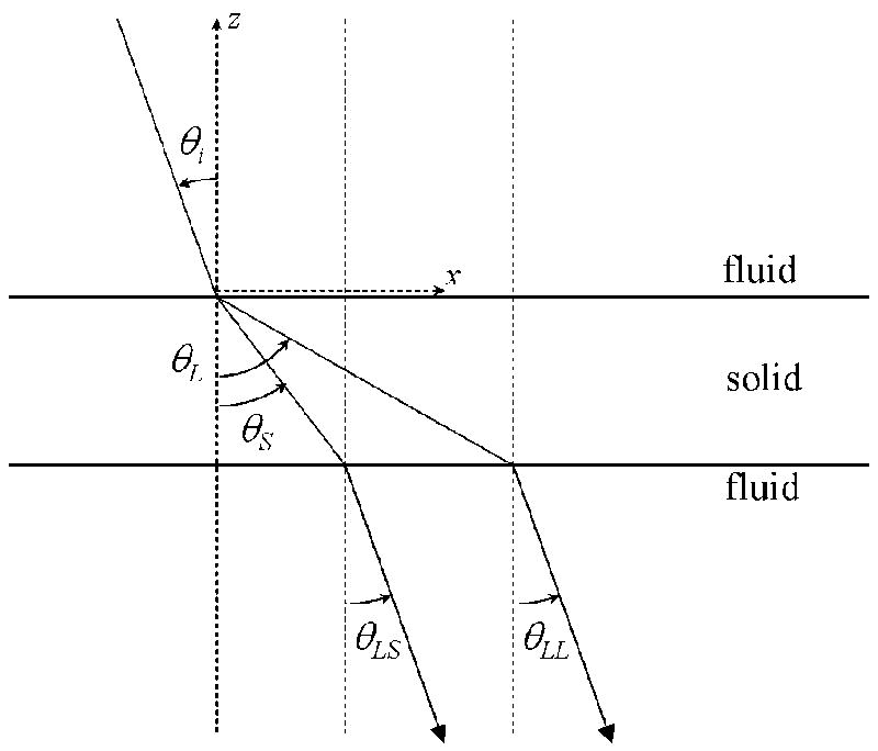
A simplified model of ultrasound transmission through the human skull. The interfaces are approximated as parallel with the Cartesian coordinates as indicated, where z is oriented orthogonal to the interfaces and x runs along the interface plane. The incident compressional wave in the fluid divides into a longitudinal and shear wave at the fluid-solid interface. At the second interface, the two propagating waves individually transmit through the interface where the shear wave is converted back to a longitudinal wave. Reflections at the interfaces are not included in the diagram or the numerical simulation.
The ultrasound transmission simulation as performed with Matlab (Mathworks, Natick, Massachusetts, USA, version 6.0.0.88 release 12) (Dell, Round Rock, Texas, USA, Inspiron 1100, Celeron 2.00 GHz) approximates the two solid-fluid interfaces as parallel boundaries and that the density between the interfaces is constant. The physical parameters used in this simulation are shown in Table 1. The fluid medium parameters were taken from the tabulated values for water (Kinsler et al. 1982a), while most of the parameters used for the solid layer were either estimates or values from another study (Fry and Barger 1978). The results of this simulation are shown in Fig. 2.
Table 1.
Parameters used for the fluid-solid-fluid acoustic intensity transmission simulation.
| Parameter | Description | Value |
|---|---|---|
| f | Sine wave frequency | 0.5 MHz |
| ρ1 | Density of water medium* | 998 kg/m3 |
| c1 | Speed of sound in water medium* | 1481 m/s |
| ρ2 | Average density of skull bone** | 1732 kg/m3 |
| c2long | Longitudinal speed of sound in skull bone** | 2850 m/s |
| c2shear | Shear speed of sound in skull bone*** | 1400 m/s |
| αlong | Longitudinal attenuation coefficient of skull bone** | 85.0 Np/m |
| αshear | Shear attenuation coefficient of skull bone*** | 90.0 Np/m |
| d | Skull bone thickness*** | 5.0 mm |
Sources: Kinsler, L. et al. (1982). Fundamentals of Acoustics, New York: John Wiley & Sons.
Fry,F.J. & Barger,J.E. Acoustical properties of the human skull. J. Acoust. Soc. Am. 63, 1576–1590 (1978).
Estimated values.
Figure 2.
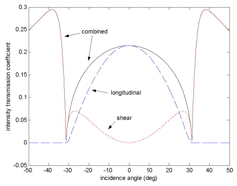
The acoustic intensity transmission coefficient as a function of incidence angle on the first interface of a two-interface model. The parameters used to create these simulated curves are shown in Table 1 and diagrammed in Figure 1.
Experiments performed to measure the longitudinal and shear speed of sound in ex vivo skull bone specimens are also described in the following section. These experimentally-obtained parameters are required for accurate analysis of the data from the power transmission measurements.
Materials and Methods
Speed of sound in skull bone
Segments from three ex vivo formalin-fixed human calvaria were stored at room temperature in an aqueous formaldehyde solution (10% buffered formalin) and submerged in deionized water for experiments (Fig. 3). The acoustic properties of formalin-fixed human calvaria are assumed to be the same as those of fresh ex vivo calvaria (Fry and Barger 1978). The water in which the experiments took place was at room temperature (measured to be 21.9±1.0 °C throughout the course of the experiments) and degassed to measure a dissolved gas content between 1 ppm and 2 ppm (Chemetrics, Calverton, Virginia, USA, CHEMet). The experimental tank was lined on all five walls with rubber, to minimize the formation of standing waves. Bone segments measuring approximately 10×10 cm were cleaved from the full calvaria specimens to facilitate measurements at high angles (~40°) in the experimental apparatus. The skull sections were mounted between a broadband plane-wave transmitting transducer (-6-dB bandwidth = 60%, 0.97-MHz center frequency, circular 12.7-mm diameter aperture) (Panametrics, Waltham, Massachusetts, USA, model V303) and a 0.2-mm diameter aperture polyvinylidene fluoride (PVDF) needle hydrophone (Precision Acoustics, Dorchester, UK, SN762) such that the incidence angle of an impinging ultrasound wave from the transmitting transducer was controlled with a precision of ±0.5° by a rotary positioning system. The outer surface of each skull fragment was positioned 50±5 mm from the face of the transmitting transducer, a distance that, for the ultrasound pulse parameters in this study, avoids the formation of standing waves between the transducer and the skull surface.
Figure 3.
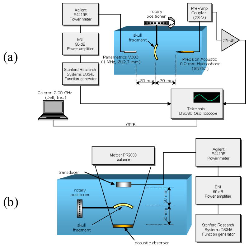
Experimental setups for measuring (A) the longitudinal and shear speed of sound and (B) the total transmitted acoustic intensity through ex vivo human skulls.
Diagrammed in Fig. 4 are the 10 locations chosen from the calvarium specimens for the transcranial ultrasound transmission study. The points were chosen based on criteria that considered as much as possible the sampling of points over the entire skull surface but limited to the geometric constraints of the experimental apparatus. In all, over the three specimens, five sonication points were located on the inferior extremities of the parietal bones (three on the right and two on the left), three points on the superior extremities of the parietal bone (all three on the left, proximal to the sagittal suture) and two were located on either side of the midsagittal line of the occipital bone. Computed tomographic (CT) scans were performed (Siemens, Munich, Germany, SOMATOM, AH82 inner ear kernel, 1-mm axial slices, 200×200-mm field-of-view) for each specimen, to characterize the inner layers of the sonicated points and to confirm the absence of trapped gases within the bone matrix. Coronal and sagittal images were constructed from the approximately 100 axial image slices per sample using an FFT interpolation technique with Matlab.
Figure 4.
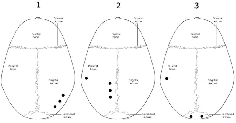
Dark spots mark the approximate locations relative to anatomical landmarks of experimental sonications on three ex vivo human calvaria. The proximity of some spots was unavoidable due to the geometric constraints of the experimental apparatus. Further limitations were imposed by the criterion that trapped gases not be present within the skull bone layers for the sonicated locations. Source: Aiello, L., Dean, C. (1990). An introduction to human evolutionary anatomy. London: Academic Press.
A pulsed sine wave (1.0 MHz, 40 cycles, PRF = 400 Hz) was generated by a function generator (Stanford Research Systems, Sunnyvale, California, USA, model DS345), amplified by 50 dB with a power amplifier (Electronic Navigation Industries, New York, USA, model 2100L) and transmitted through each of the 10 locations on the skull specimens and received by the needle hydrophone situated 120 mm from the ultrasound source. The total power transmission (0.6 W) was monitored by a power meter (Agilent, Palo Alto, California, USA, model E4419B) placed in parallel between the power amplifier and the submerged transducer. The waveform as registered by the hydrophone was amplified by 25 dB (Precision Acoustics, Dorchester, UK), recorded by a digital oscilloscope (Tektronix, Beaverton, Oregon, USA, model TDS380), and transferred to a computer (Dell, Round Rock, Texas, USA, Inspiron 1100, Celeron 2.00 GHz) for analysis.
Transmitted waveforms through each of the 10 points were obtained for normal incidence and 40° incidence of the ultrasound pulse with the outer surface of the skull. Forty degrees was determined a posteriori with the measured sound speeds to be beyond the maximum angle for longitudinal wave transmission through the skull. This calculation confirmed that any detected ultrasound waves at 40° incidence were purely due to shear mode propagation in the skull. A reference waveform was also obtained by transmitting the pulse through water without an intervening skull layer.
The recorded waveforms consisted of 1000 samples over 10 μs, giving a time resolution of 10 ns and time delayed by 74.7 μs to account for acoustic time-of-flight. For each of the 10 locations that were sonicated, a time-of-flight comparison was made by observing the arrival time of the second prominent maximum of the signal (Fig. 5). The second peaks were selected for analysis, because the first peaks, although observable in every instance, provided a less accurate time determination, due to their lower levels. The speed of sound through the intervening skull layer, cB, averaged over the entire thickness, was calculated according to
Figure 5.
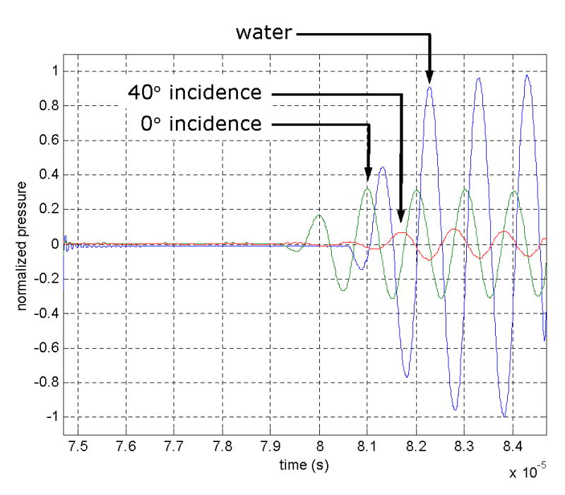
Time plots of a 1.0-MHz sinusoidal pulse propagated through a skull layer at normal incidence (0°), 40° incidence, and a third without an intervening skull layer (“water”). The arrows indicate the peaks selected for time-of-flight analysis. The pressure levels are normalized to the peak-to-peak value of the water transmission waveform. Note that the time scale has a 10−5 multiplicative factor as indicated at the lower right of the graph.
| (1) |
where d is the skull thickness as measured by a digital caliper (Mitutoyo, Kawaski, Japan, model CD-6) at the sonication location, θi is the incidence angle of the ultrasound path with the outer surface of the skull, tW is the calculated time-of-flight through a layer of water of thickness d cos (θi) using the tabulated water sound speed (Kinsler et al. 1982a) of 1481 m/s and Δt is the measured time difference between the second prominent peaks of the ultrasound pulse, with and without an intervening skull bone layer. The calculated sound speeds were then categorized as a longitudinal (θi = 0°) or shear (θi = 40°) sound speed.
Ultrasound energy transmission
To examine ultrasound energy transmission through human skull bone in the longitudinal and shear modes, the skull segments of the previous section were aligned in the experimental set-up (Fig. 3) such that the same locations as those diagrammed in Fig. 4 were exposed to the transmitting ultrasound beam. It was determined through examination of CT images that these sections of the skull bone did not contain trapped gases or other defects that would have interfered with a realistic assessment of ultrasonic properties. As diagrammed in Fig. 3, the individual skull fragments were mounted such that the sonicated location was equidistant from the source transducer and the acoustic absorber. Affixed to a rotary positioner (precise to ±0.5°), the skull was positioned manually to vary the incidence angle between its outer surface and the ultrasound beam path. Two in-house-manufactured air-backed transducers (referred to from here on as transducer A and transducer B) transmitted sine waves of frequencies 0.272 MHz (fundamental thickness mode of transducer A), 0.548 MHz (fundamental thickness mode of transducer B) and 0.840 MHz (third harmonic of transducer A). Both transducers consisted of gold-plated lead-zirconate-titanate (PZT) and were spherically focused, with an active-area diameter of 50 mm and a 100-mm radius-of-curvature. For optimal transduction, the input impedance of each transducer for each operating frequency was matched with passive LC-circuitry.
The acoustic absorber consisted of frayed polymer bristles which were bundled such that the closely packed tips acted as point scatterers, deflecting most of the energy into the brush, where it becomes absorbed (Hynynen 1993). Sources of systematic experimental error stemmed from unavoidable obstacles in the vicinity of the set-up that potentially interacted with the acoustic field. These included the thin nylon strings that held the acoustic absorber, the walls of the tank and support structures for positioning the skull. The water-air interface of the water surface was also a potential reflector of errant acoustic energy. Measures were taken to minimize the effects of these structures. Ultrasound absorbing silicone layers (General Electric Silicones, Wilton, Connecticut, USA, RTV108) were applied as coatings on many reflective surfaces and extra layers of acoustically absorbing materials were attached to the walls of the tank.
To measure the incident angle dependency of the total ultrasound power transmitted through the skull bone, a continuous-wave sine function was transmitted through each of the 10 locations on the skull fragments and the angle of incidence was varied in 1° increments. At each angle of incidence and for each of the three sonicating frequencies, the force exerted on the acoustic absorber, which is proportional to the total transmitted acoustic power, was recorded. The total electrical power for all sonications was monitored by a power meter (Agilent, Palo Alto, California, USA, model E4419B) coupled to the transmitted signal by a dual-directional coupler (Werlatone, Brewster, New York, USA, model 01373). Each sonication of approximately 3 s duration was held constant at 32 We (electrical watts) and 10 s were allowed to elapse between sonications, to allow for cooling of the bone fragment and of the absorbing brush. For the transducers used in this study, 32 We was measured to be the equivalent of 22 Wa (acoustic watts) for 0.272-MHz sonications, 24 Wa for 0.548-MHz sonications and 21 Wa for 0.840-MHz sonications). This radiation force measurement was also performed for each frequency without a skull, to establish a baseline to be used in the analysis.
Nonlinear effects were determined to be negligible, as the shock distances in water for the sonication parameters were calculated to be at least 1.2 m for 0.272 MHz, 0.9 m for 0.548 MHz and 0.8 m for 0.840 MHz. These distances, determined for spherically focused waves (Bacon 1984), were substantially greater than the length scales of the experimental set-up. For experimental confirmation, the harmonic content of a 21-Wa, 0.840-MHz signal at a distance of 400 mm along the axis of the transducer was determined from pressure measurements with a 0.2-mm diameter PVDF needle hydrophone. The results, shown in Fig. 6, demonstrated observable harmonics with pressure levels as high as 20% of that of the fundamental. But, assuming a linear decrease in harmonic content as one approaches the transducer face (Pierce 1989), the pressure level of each harmonic was calculated to be less than 3% that of the fundamental at the skull surface. As this calculation was for the worst-case scenario (i.e., highest frequency), the effect of nonlinear propagation for each case in this study was deemed to be negligible.
Figure 6.
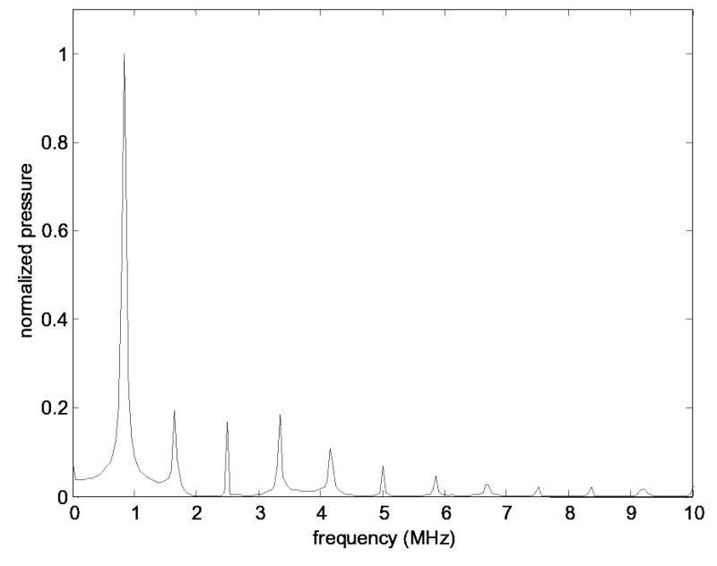
The measured spectrum for the propagation of a 0.840-MHz converging wave at 21 Wa for a distance of 400 mm in degassed deioinized water. The presence of nonlinear higher harmonic formation is evident.
The radiation force as exerted on an acoustic absorber from ultrasound energy transmitted through skull bone was measured over the entire spatial extent of the ultrasound beam width. This was especially important in the case of nonnormal angles of incidence at the bone interface and nonparallelisms in the bone interfaces.
To obtain an estimate of the bone properties that could produce the results of the radiation force measurements, the one-dimensional single-layer simulation of Fig. 2 was performed with new parameters, with the intent of comparing the simulations with the data from each measured location. The objective of the new simulation was to generate a transmission curve that most closely matched the measured transmission for the three frequencies in question at normal incidence (pure longitudinal) and at 38° incidence (pure shear). The initial set of new parameters included the frequency, bone density, longitudinal sound speed, shear sound speed and skull thickness. Bone density values used for each simulated transmission were extrapolated from a spatial average of CT image Hounsfield units for each sonicated cross-section on the specimens. Longitudinal and shear sound speed values, along with the corresponding skull thickness values, were used in the simulations. Measured transmission curves for each point were matched to simulations at normal incidence and at 38° incidence, to obtain attenuation estimates. This analysis was performed for each of the three measured frequencies.
Results
Speed of sound in skull bone
The average measured speed of sound for a 1.0-MHz longitudinal wave propagated through 10 points over three ex vivo human calvaria was 2820±40 m/s. The average measured speed of sound for a 1.0-MHz shear wave propagated through 10 points over three ex vivo human calvaria was 1500±140 m/s. These results are plotted in Fig. 7 and are used in the analysis of radiation force measurements of incidence angle dependent acoustic power transmission.
Figure 7.
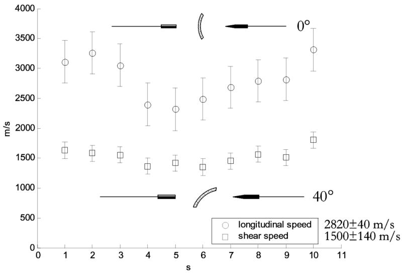
Longitudinal and shear mode sound speeds as measured through ten locations over three ex vivo human calvaria specimens. The experiments were performed with pulsed 1.0-MHz sine waves with pulse repetition frequencies (PRF) of 400 Hz. The mean longitudinal sound speed is 2820±40 m/s and the mean shear sound speed is 1500±140 m/s.
Ultrasound energy transmission
Figure 8 contains a sample plot for transmission through one skull sample from the series of radiation force measurements of incidence-angle-dependent acoustic power transmission. The transmitted acoustic power as a percentage of transmission without the skull is plotted as a function of the incidence angle with the first interface of the skull bone. The CT image of the point being sonicated is also shown, verifying the absence of trapped gases that would interfere with the measurements. In addition to the observable transmission peaks near normal incidence, there was a slight increase in the measured radiation force for incidence angles past 30° for the frequencies 0.272 MHz and 0.548 MHz. For the 0.272-MHz case, the power transmission minimum occurred at 28° incidence, where the measured force was 36% of the value at normal incidence, and then it increased to 42% at 42°. For 0.548 MHz, the minimum was observed at 31° from normal incidence, where it was 33% of the value at normal incidence; beyond that, it increased to 50% at 49°.
Figure 8.
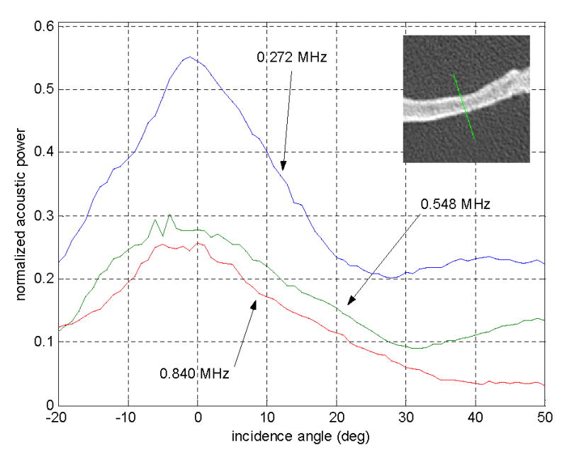
Transmitted ultrasound intensity as measured by the radiation force on an acoustic absorber. The three curves are the measurements for three frequencies from one sonication point on an ex vivo human skull as a function of incidence angle on the outer surface of the skull. The measurements were taken in 1° intervals and the CT image of the sonicated point is shown at the upper right. The values were normalized to the measured radiation force of the same frequencies propagated through water (i.e. no skull).
The power transmission data for all 10 points were averaged to produce three curves, one for each frequency (Fig. 9). The averaged data for 0.272-MHz, 0.548-MHz and 0.840-MHz transmissions had maximum values at incidence angles of −1°, −2° and 1°, respectively. The percentages of acoustic power transmitted at each frequency for normal incidence are tabulated in Table 2. At its minimum, the power transmission for 0.272 MHz was 18% of the incident acoustic power. This was 47% of the peak transmission value at −1° incidence.
Figure 9.
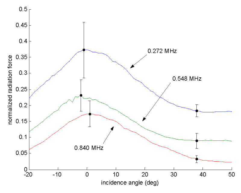
Transmitted ultrasound intensity as measured by the radiation force on an acoustic absorber. The three curves are the average values for measurements taken over ten sonication points on three ex vivo human calvaria. The values were normalized to the measured radiation force of the same frequencies propagated through water (i.e. no skull).
Table 2.
The percentage of acoustic power transmitted via a longitudinal mode (normal incidence) and a shear mode (38° incidence) as averaged over ten samples.
| Frequency (MHz) | Average longitudinal transmission (%) | Average shear transmission (%) |
|---|---|---|
| 0.272 | 37±9 | 18±2 |
| 0.548 | 23±5 | 9±2 |
| 0.840 | 17±4 | 3±1 |
The averaged measured frequency curves are shown in Fig. 10, with their respective fitted-parameter simulations. The longitudinal and shear attenuation values obtained by fitting the simulated transmission curves with each measured transmission curve are presented in Table 3 and in Fig. 11.
Figure 10.
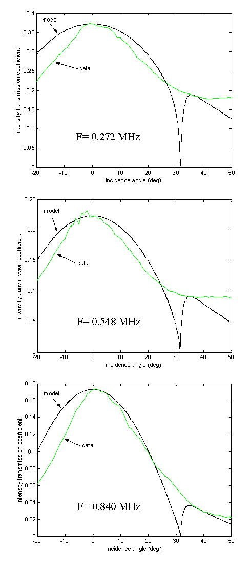
Measured ultrasound intensity transmission (averaged over ten points) and simulated intensity transmission through a bone layer over a series of incident angles for the frequencies 0.272-MHz, 0.548-MHz, and 0.840-MHz.
Figure 11.

Attenuation values for both the longitudinal and shear mode of wave propagation in skull bone. These values were obtained through a combination of measured data and comparisons of measurements with simulated data.
Discussion
Experimental studies of the ultrasound propagation properties of human tissue include, among others, those of propagation through the skull in longitudinal mode (Fry and Barger 1978), shear mode propagation in soft tissue (Frizzell and Carstensen 1976) and guided waves in long weight-bearing bones (Tatarinov et al. 2005). The measurements performed in this study on the properties of pure shear mode propagation through the skull bone synthesizes these types of measurements to provide a set of data that is more specific and much needed in the continuing study of transcranial ultrasound transmission.
The experimental evidence, in conjunction with simplified one-dimensional models, demonstrated that the shear attenuation coefficient in skull bone was on average higher by 115 Np/m than the longitudinal attenuation coefficient for the frequency range studied (0.272 MHz to 0.840 MHz). So although the closer match in characteristic impedance to the surrounding medium allowed for more efficient transmission through the boundaries, the skull bone’s intrinsic attenuation of ultrasound energy in shear mode overshadowed this impedance matching effect.
The simplification of the model for interfacial transmission was possibly the most significant source of error for the derivation of bone propagation parameters. Future studies in ultrasound transmission through the skull would benefit from a more extensive and thorough consideration of the geometric parameters and the nonlinear possibilities of transcranial ultrasound propagation.
Conclusion
The results of this study give indication that an induced shear mode in the skull bone for therapeutic applications will likely exacerbate the bone heating problem, since the energy attenuation, likely due largely to absorption, is higher in the skull bone for the shear mode as compared to the longitudinal mode. But the data also show that a pure transcranial shear mode does exist. And since a shear mode is less distorting than the longitudinal mode, an advantage can exist for imaging applications. Further studies are being planned to determine the efficacy of using the transcranial shear mode for noninvasive brain imaging.
Table 3.
Longitudinal and shear attenuation of human skull bone determined by fitting simulations to measured values
| Frequency (MHz) | Longitudinal attenuation (Np/m) | Shear attenuation (Np/m) |
|---|---|---|
| 0.272 | 14±17 | 94±24 |
| 0.548 | 53±43 | 146±36 |
| 0.840 | 70±28 | 213±42 |
Acknowledgments
This work was supported by grant R21EB004353 and U41RR019703 from the National Institutes of Health
Appendix: transmission theory
In its simplest one-dimensional form, Hooke’s law can be written as
| (2) |
where, for small displacements in an elastic system, k is the constant of proportionality between an applied force, F, and the resulting displacement, x. In three dimensions, this relationship is expanded to
| (3) |
where the applied force is now represented by the stress tensor σij, whose elements represent the combination of forces acting in the three spatial directions at a point. The resulting displacement is represented by the strain tensor ɛkl, whose elements represent the spatial deformation of the body on which the force is acting. The constants of proportionality between the stress and strain tensors are the elements of cijkl, a fourth-rank tensor also known as the elastic constant tensor. The notational convention is such that each index (i, j, and k) represents one of three spatial directions (x, y, and z) such that σij and ɛkl each have nine elements and cijkl has 81 elements in order to express the elastic relationship completely. By convention, the first indices of the stress and strain tensors represent the direction in which the force acts or the direction of deformation, respectively. The second indices of the stress and strain tensors indicate the direction orthogonal to the plane on which the force is acting or the direction orthogonal to plane that is invariant under this deformation, respectively. It has been well established (Kittel 1996) through physical principles of symmetry that the elements of cijkl can be reduced to two independent elastic constants for isotropic solids, which is the approximation that will be used in this model. In fact,
| (4) |
where λ and μ are the physical parameters otherwise known jointly as the Lamé constants of the material. The Kronecker delta, δij, as used in Eq. (4) with different combinations of indices, is a mathematical device defined as
| (5) |
such that the elements of cijkl are all linear combinations of λ and μ. Using Eqs. (3–5), the relation between the stress tensor elements and the strain tensor elements for isotropic solids can written as
| (6) |
for the longitudinal wave parameters (the “diagonal” elements of the elastic constant tensor), and
| (7) |
for the shear wave parameters (the “off-diagonal” elements of the elastic constant tensor). Using the conventions of Figure 1 and the definition of the velocity potential in a fluid,
| (8) |
and in a solid,
| (9) |
where the particle velocity fields are represented by gradients of the scalar functions Φ and Θ, and the curl of a vector field , the solution to the wave equation can be expressed as such:
| (10) |
| (11) |
| (12) |
and
| (13) |
In order to describe a physically realizable system that is consistent with the conventions as set up by Figure 1, Ψ in Eq. (13) is defined as the y-component of such that the velocity field in Eq. (9) will have nonzero components only in the xz-plane. These equations describe the single-interface fluid-to-solid scenario where TL and TS are acoustic transmission coefficients for the propagated longitudinal and shear waves in the solid, respectively. The scalar fields Φi, Φr, Θ, and Ψ represent the incident wave, the reflected wave, the transmitted longitudinal wave, and the transmitted shear wave, respectively, and are valued in the xz-plane (with the exception of Ψ, as described earlier) and in t. Equation (11), although not included in the simulation study, is presented for completeness. It contains the acoustic reflection coefficient, R, and other parameters of the wave that is reflected from the interface. The wave numbers for the longitudinal acoustic waves in the fluid and solid are kf and kL, respectively, and the wave number for the shear wave in the solid is kS. The angular frequency is ω.
Now that the stress-strain relationships have been established and a wave equation solution has been stated that is in accordance to the conventions as set up by Figure 1, some mathematical manipulations are performed to provide relations to be combined with boundary conditions. This will lead to a solution for the transmission coefficients of Eqs. (12–14) in terms of physical parameters of the system. Combining the definition of strain, which is
| (14) |
where is the particle displacement, and the stress-strain relations of Eqs. (6–7),
| (15) |
and
| (16) |
Exchanging the displacements with velocities, for time harmonic waves, Eqs. (15–16) become
| (17) |
and
| (18) |
Using the definition of the velocity potential, Eq. (9), we can redefine vx and vz in Eqs. (17–18) as
| (19) |
and
| (20) |
Partial derivatives with respect to y were set to zero since the velocity field components are confined to the xz-plane. This leads to a useful formulation to be used with boundary conditions:
| (21) |
and
| (22) |
The boundary conditions for the fluid-solid interface include continuity of normal velocities, continuity of normal stresses, and a zero tangential stress component to accommodate the incompatibility of a nonzero tangential force with an ideal fluid. These conditions are given mathematically as
| (23) |
and
| (24) |
where λf is the Lamé constant for fluid, while the λ and μ without subscripts are the Lamé constants for the solid. The disappearing of tangential stress is given by
| (25) |
The substitution of these three boundary conditions into Eqs. (10–13) will first yield Snell’s law
| (26) |
where cf and cL are the longitudinal sound speeds in fluid and solid, respectively, and cS is the shear sound speed in the solid. These were obtained using the relations
| (27) |
and
| (28) |
Theses relations, along with the boundary conditions, can be further combined with the wave equation solutions to obtain three equations:
| (29) |
| (30) |
and
| (31) |
where ρf and ρs refer to the densities of the fluid and the solid, respectively. Solving for the pressure transmission coefficients,
| (32) |
and
| (33) |
where
| (34) |
| (35) |
and
| (36) |
The values obtained by this analysis are then used as the input for the next interface, for which a similar approach is taken to determine the transmission coefficient for the solid-fluid interface.
As a function of angle from −50° to 50°, the intensity transmission coefficients for the longitudinal wave, TL, and the shear wave, TS, through the bone are presented. The sum of these values are also plotted and labeled as a combined intensity transmission coefficient. The acoustic intensity transmission coefficients were obtained by the definition
| (37) |
which, for harmonic plane waves, can be written
| (38) |
When applied to the present simulation, for one interface,
| (39) |
and
| (40) |
Substituting the cosine terms with the trigonometric identity
| (41) |
and normalizing the results to the incident acoustic intensity by setting Ii = 1, Eqs. (30–40) can be written
| (42) |
and
| (43) |
By recognizing that Snell’s Law gives
| (44) |
Eqs. (42–43) can be simplified to
| (45) |
and
| (46) |
Finally, an attenuation factor for the bone medium is included in the form of
| (47) |
where I0 is the transmission intensity from Eqs. (45) and (46), d is the solid layer thickness, and α is the attenuation coefficient in nepers per meter. The introduction of this ad hoc attenuation factor in the final stage of the simulation was for the purpose of estimating an attenuation value for longitudinal and shear waves in the skull by comparison with measured data. An artificial dip in transmission at the critical angle is preserved by using this method. The values for Eqs. (45) and (46) after the inclusion of individual estimated attenuation coefficients are shown in Figure 2 for θi ranging from −50° to 50° at a resolution of 1°. The combined predicted acoustic intensity transmission, I L + IS, is also plotted along with the longitudinal and shear transmissions.
Footnotes
Ultrasound modes through skull bone
References
- Bacon DR. Finite amplitude distortion of the pulsed fields used in diagnostic ultrasound. Ultrasound Med Biol. 1984;10:189–195. doi: 10.1016/0301-5629(84)90217-5. [DOI] [PubMed] [Google Scholar]
- Behrens S, Spengos K, Daffertshofer M, Schroeck H, Dempfle CE, Hennerici M. Transcranial-ultrasound-improved thrombolysis: diagnostic vs. therapeutic ultrasound. Ultrasound Med Biol. 2001;27:1683–1689. doi: 10.1016/s0301-5629(01)00481-1. [DOI] [PubMed] [Google Scholar]
- Carson PL, Oughton TV, Hendee WR, Ahuja AS. Imaging soft tissue through bone with ultrasound transmission tomography by reconstruction. Med Phys. 1977;4:302–309. doi: 10.1118/1.594318. [DOI] [PubMed] [Google Scholar]
- Cheeke J. D. N. (2002) Reflection and transmission of ultrasonic waves at interfaces, in Fundamentals and applications of ultrasonic waves pp. 115–142. CRC Press, Boca Raton.
- Clement GT, Sun J, Hynynen K. The role of internal reflection in transskull phase distortion. Ultrasonics. 2001;39:109–113. doi: 10.1016/s0041-624x(00)00052-4. [DOI] [PubMed] [Google Scholar]
- Clement GT, White PJ, Hynynen K. Enhanced ultrasound transmission through the human skull using shear mode conversion. J Acoust Soc Am. 2004;115:1356–1364. doi: 10.1121/1.1645610. [DOI] [PubMed] [Google Scholar]
- Daum DR, Buchanan MT, Fjield T, Hynynen K. Design and evaluation of a feedback based phased array system for ultrasound surgery. IEEE Trans Ultrason Ferroelectr Freq Contr. 1998;45:431–438. doi: 10.1109/58.660153. [DOI] [PubMed] [Google Scholar]
- Dines KA, Fry FJ, Patrick JT, Gilmor RL. Computerized ultrasound tomography of the human head: experimental results. Ultrason Imaging. 1981;3:342–351. doi: 10.1177/016173468100300404. [DOI] [PubMed] [Google Scholar]
- Frizzell LA, Carstensen EL. Shear properties of mammalian tissues at low megahertz frequencies. J Acoust Soc Am. 1976;60:1409–1411. doi: 10.1121/1.381236. [DOI] [PubMed] [Google Scholar]
- Fry FJ. Transkull transmission of an intense focused ultrasonic beam. Ultrasound Med Biol. 1977;3:179–184. doi: 10.1016/0301-5629(77)90069-2. [DOI] [PubMed] [Google Scholar]
- Fry FJ, Barger JE. Acoustical properties of the human skull. J Acoust Soc Am. 1978;63:1576–1590. doi: 10.1121/1.381852. [DOI] [PubMed] [Google Scholar]
- Fry F. J., Eggleton R. C., and Heimburger R. F. (1974) Transkull visualization of brain using ultrasound; an experimental model study. Exerpta Medica 97–103.
- Hayner M, Hynynen K. Numerical analysis of ultrasonic transmission and absorption of oblique plane waves through the human skull. J Acoust Soc Am. 2001;110:3319–3330. doi: 10.1121/1.1410964. [DOI] [PubMed] [Google Scholar]
- Hynynen K. Acoustic power calibrations of cylindrical intracavitary ultrasound hyperthermia applicators. Med Phys. 1993;20:129–134. doi: 10.1118/1.597094. [DOI] [PubMed] [Google Scholar]
- Hynynen K, Jolesz FA. Demonstration of potential noninvasive ultrasound brain therapy through an intact skull. Ultrasound Med Biol. 1998;24:275–283. doi: 10.1016/s0301-5629(97)00269-x. [DOI] [PubMed] [Google Scholar]
- Hynynen K, McDannold N, Vykhodtseva N, Jolesz FA. Noninvasive MR imaging-guided focal opening of the blood-brain barrier in rabbits. Radiology. 2001;220:640–646. doi: 10.1148/radiol.2202001804. [DOI] [PubMed] [Google Scholar]
- Kinsler L. E., Frey A. R., Coppens A. B., and Sanders J. V. (1982a) Fundamentals of acoustics, John Wiley & Sons, New York.
- Kinsler L. E., Frey A. R., Coppens A. B., and Sanders J. V. (1982b) Transmission phenomena, in Fundamentals of Acoustics pp. 124–140. John Wiley & Sons, New York.
- Kirkham FJ, Padayachee TS, Parsons S, Seargeant LS, House FR. Transcranial measurement of blood flow velocities in the basal cerebral arteries using pulsed Doppler ultrasound. Ultrasound Med Biol. 1986;12:15–21. doi: 10.1016/0301-5629(86)90139-0. [DOI] [PubMed] [Google Scholar]
- Kittel C. (1996) Crystal binding and elastic constants, in Introduction to solid state physics pp. 53–96. John Wiley & Sons, New York.
- Lynn JG, Zwemer RL, Chick AJ, Miller AE. A new method for the generation and use of focused ultrasound in experimental biology. J Gen Physiol. 1942;26:179–193. doi: 10.1085/jgp.26.2.179. [DOI] [PMC free article] [PubMed] [Google Scholar]
- Pierce A. D. (1989) Acoustics, an introduction to its physical principles and applications, Acoustical Society of America, Woodbury.
- Postert T, Hoppe P, Federlein J, Przuntek H, Buttner T, Helbeck S, Ermert H, Wilkening W. Ultrasonic assessment of brain perfusion. Stroke. 2000;31:1460–1462. doi: 10.1161/01.str.31.6.1457-b. [DOI] [PubMed] [Google Scholar]
- Smith S. W., Phillips D. J., von Ramm O. T., and Thurstone F. L. (1979) Some advances in acoustic imaging through the skull. Nat Bur Standards Pub #525 209–218.
- Sun J, Hynynen K. The potential of transskull ultrasound therapy and surgery using the maximum available skull surface area. J Acoust Soc Am. 1999;105:2519–2527. doi: 10.1121/1.426863. [DOI] [PubMed] [Google Scholar]
- Tanter M, Thomas JL, Fink M. Focusing and steering through absorbing and aberrating layers: application to ultrasonic propagation through the skull. J Acoust Soc Am. 1998;103:2403–2410. doi: 10.1121/1.422759. [DOI] [PubMed] [Google Scholar]
- Tatarinov A, Sarvazyan N, Sarvazyan A. Use of multiple acoustic wave modes for assessment of long bones: model study. Ultrasonics. 2005;43:672–680. doi: 10.1016/j.ultras.2005.03.004. [DOI] [PMC free article] [PubMed] [Google Scholar]
- Tobias J, Hynynen K, Roemer R, Guthkelch AN, Fleischer AS, Shively J. An ultrasound window to perform scanned, focused ultrasound hyperthermia treatments of brain tumors. Med Phys. 1987;14:228–234. doi: 10.1118/1.596074. [DOI] [PubMed] [Google Scholar]
- Ylitalo J, Koivukangas J, Oksman J. Ultrasonic reflection mode computed tomography through a skull bone. IEEE Trans Biomed Eng. 1990;37:1059–1066. doi: 10.1109/10.61031. [DOI] [PubMed] [Google Scholar]