Dual-Color Time-Integrated Fluorescence Cumulant Analysis

Abstract

We introduce dual-color time-integrated fluorescence cumulant analysis (TIFCA) to analyze fluorescence fluctuation spectroscopy data. Dual-color TIFCA utilizes the bivariate cumulants of the integrated fluorescent intensity from two detection channels to extract the brightness in each channel, the occupation number, and the diffusion time of fluorophores simultaneously. Detecting the fluorescence in two detector channels introduces the possibility of differentiating fluorophores based on their fluorescence spectrum. We derive an analytical expression for the bivariate factorial cumulants of photon counts for arbitrary sampling times. The statistical accuracy of each cumulant is described by its variance, which we calculate by the moments-of-moments technique. A method that takes nonideal detector effects such as dead-time and afterpulsing into account is developed and experimentally verified. We perform dual-color TIFCA analysis on simple dye solutions and a mixture of dyes to characterize the performance and accuracy of our theory. We demonstrate the robustness of dual-color TIFCA by measuring fluorescent proteins over a wide concentration range inside cells. Finally we demonstrate the sensitivity of dual-color TIFCA by resolving EGFP/EYFP binary mixtures in living cells with a single measurement.

INTRODUCTION

Fluorescence fluctuation spectroscopy (FFS) examines the fluctuating fluorescence signal from a small illumination volume <1 fl created by modern two-photon or confocal microscopy (1,2) to characterize the behavior of fluorophores. Statistical analysis tools such as fluorescence correlation spectroscopy (3) and photon-counting histogram (PCH) or fluorescence intensity distribution analysis (4,5) are required to extract static and dynamic information from the stochastic fluorescence signal. Fluorescence correlation spectroscopy uses the correlation function to capture the temporal information of the physical process, while PCH uses the amplitude distribution of the fluctuations to characterize the concentration and brightness of each fluorescent species. Fluorescence intensity multiple distribution analysis (6) and photon arrival-time interval distribution (7) have been developed to take both temporal and amplitude information into account. A PCH theory that incorporates diffusion has also recently been described (8).

Moment analysis is an alternative technique for studying a fluctuating fluorescence signal and was originally developed in the late 80s and early 90s (9–12). Fluorescent cumulant analysis (FCA) (13) and time-integrated fluorescence cumulant analysis (TIFCA) (14) represent a further development of moment analysis. Cumulants are a special representation of moments that possess mathematical properties particularly suited for statistical analysis. For example, cumulants of independent random variables are additive. We previously discussed the advantages of using cumulants in analyzing fluorescence fluctuation data (13,14). FCA uses simple analytical expressions that relate the factorial cumulants of the photon counts to the molecular brightness and occupation number in the observation volume. TIFCA generalizes the cumulant analysis to arbitrary sampling times, which makes it able to determine the dynamics as well as the concentration of fluorescent species. The exact theoretical treatment of TIFCA also allows the optimization of signal statistics in the analysis of FFS experiments.

In conventional FFS, all light is collected by a single detector. In most two-channel FFS experiments, the fluorescent signal is split by a dichroic mirror into two different detectors based on the color of the fluorophore. Two-channel FFS offers the possibility to resolve fluorophores according to their emission spectra, thus offering a method for detecting the association and dissociation between different species of biomolecules (15–17). The sensitivity of two-channel FFS in resolving species is dramatically improved over conventional single-channel FFS. In this article, we extend the theory of TIFCA to two-channel FFS experiments. A simple expression for the bivariate factorial cumulant of photon counts is derived for arbitrary binning times. Theoretical models are used to fit the experimental cumulants of the photon counts as a function of sampling time, which simultaneously determines the molecular brightness in each channel, the occupation number, and the diffusion time of each species from a single measurement. The statistical error of factorial cumulants is also derived and experimentally verified. The relative error of cumulants measures its statistical significance and provides weighting factors for data fitting.

Nonideal detector effects cause artifacts in the analysis of FFS data (18,19). These effects, if not accounted for, may lead to erroneous interpretation of the experimental data and therefore severely limit the practical use of the analysis technique. We develop in this article a theoretical model of nonideal detector effects on the factorial cumulants of photon counts and verify it experimentally.

The new technique is then applied to study EGFP and EYFP in living cells. We first measure EGFP and EYFP alone to demonstrate the validity of the theory in this challenging environment. The EGFP/EYFP pair exhibits strong spectral overlap, which poses a serious challenge for resolving species by FFS (17). Based on the parameters determined from the single-species measurements of EGFP and EYFP, we investigate the resolvability of the two proteins theoretically. Our results show a dramatic improvement of resolvability compared to conventional PCH analysis. Finally, we apply dual-color TIFCA to resolve for the first time binary mixtures of EGFP and EYFP over a wide concentration range from single measurements in living cells.

THEORY

Cumulants for arbitrary binning times

The derivation of dual-color cumulant analysis closely follows that of regular TIFCA (14). Since regular TIFCA theory only considers a single detection channel, we also refer to it as single-color or single-channel TIFCA. In the dual-color case, the fluorescence light is split into two different detectors with a dichroic mirror. A theory that describes the bivariate factorial cumulants of photon counts detected in two channels is needed. Here, we use the labels A and B to distinguish the two detection channels and the subscript Q refers to any one of the two channels. As a convention in this article, channel A always refers to the red channel and channel B to the blue channel. The probability distribution function P(k_A,k_B;T) of detecting k_A photons in channel A and k_B photons in channel B is related to the probability distribution function P(W_A,W_B) of the integrated light intensity W_A and W_B, according to Mandel's formula (20),

(1)

where η_A and η_B are the detection efficiencies of the photon detectors and T is the sampling time. For convenience, we set η_A = η_B = 1, which is equivalent to measuring the intensity in counts per second (cps). As a convention, we use κ_m,n as a symbol for the (m,n)^th cumulant and κ_[m,n] for the (m,n)^th factorial cumulant. An up-carat (^) over a symbol indicates that it represents an experimentally measured physical quantity. Mandel's formula implies that the bivariate cumulant generating function of (W_A,W_B) equals the bivariate factorial cumulant generating function of (k_A, k_B). In other words, the cumulant κ_m,n(W_A,W_B) of the integrated intensity (W_A, W_B) is determined experimentally by measuring the corresponding factorial cumulant κ_[m,n](k_A, k_B) of the photon counts (k_A,k_B),

(2)

Next, we calculate the theoretical expression of κ_m,n(W_A,W_B) for arbitrary sampling times T. Assume that a single molecule is diffusing in a large, but closed volume V illuminated by focused laser light with a normalized point spread function (PSF) given by . The experimental PSF is approximated by a model function. Usually a three-dimensional Gaussian is used in the literature to describe the PSF of fluorescence fluctuation spectroscopy,

(3)

where s refers to an s-photon (s = 1,2…) excitation experiment. The same PSF can be used for both detection channels since the fluorophores are coexcited by the same laser. When the molecule is located at position at time t, the fluorescence intensity I_Q in channel Q (Q = A, B) is given by

(4)

where λ_Q (measured in counts per second per molecule, i.e., cpsm) is the brightness of fluorophores in channel Q. The integrated intensity W_Q within the sampling time T is

(5)

With the above definition, the (m,n)^th bivariate raw moment of (W_A,W_B) is easily calculated as

(6)

The above integration has been solved and is expressed in terms of binning functions B_m+n(T;τ_d) in Wu and Müller (14),

(7)

where V_PSF is the reference volume conventionally used in fluorescent fluctuation experiments,

(8)

and the coefficient γ_s is called the s^th γ-factor and defined as

(9)

According to Wu and Müller (14), the binning function only depends on the diffusion time τ_d = w²/4sD for a molecule with diffusion constant D in a focused laser beam with beam waist w. The binning function depends on the choice of PSF and has been previously determined for a three-dimensional Gaussian PSF (14). Because the excitation profile of both detection channels overlaps, only a single PSF is needed.

The (m,n)^th bivariate cumulant of (W_A,W_B) can be expressed as a series of terms of raw moments up to (m,n)^th order, where denotes the (m,n)^th cumulant for a single molecule. In the thermodynamic limit V → ∞, all terms except the (m,n)^th raw moment vanish (13),

(10)

Now suppose there are N_total noninteracting, diffusing molecules in the volume V, such that in the thermodynamic limit V → ∞, the concentration c = N_total/V is kept constant. We define the average occupation number N in the observation volume V_PSF,

(11)

Since the fluorescence emitted by different noninteracting molecules is statistically independent from each other, the cumulant of the total integrated fluorescence intensities in the two channels is given by summing up the corresponding cumulant of all individual molecules,

(12)

In the short sampling time limit T ≪ τ_d, the binning function B_m+n(T;τ_d) is approximated by T^m+n (14). In this limit the bivariate cumulant simplifies to

(13)

The cumulants of a mixture of noninteracting fluorescent species are given by the sum of the cumulants of each individual species according to the additive property of cumulants for independent random variables,

(14)

Experimentally, photon counts are observed instead of integrated intensities. Equation 2 allows us to measure the cumulants of the integrated intensities κ_m,n(W_A, W_B) by calculating the experimental estimates of the factorial cumulant of the photon counts κ_[m,n] (k_A, k_B).

Variance of the bivariate factorial cumulants

The variance of an experimental quantity is an important measure of its statistical accuracy. In fluorescence cumulant analysis, the variance of the factorial cumulant is used as the weight in the nonlinear least-squares fit to the theoretical model. The variance is also a good indicator of how many statistically significant cumulants are present in the data. It is difficult to exactly calculate the variance of multivariate factorial cumulants of experimental photon counts with a finite number of correlated data points. We use a technique called moments-of-moments, which ignores the correlation in the data, to calculate the variance of the factorial cumulant. A detailed discussion of the limitations of this technique has been presented for the univariate case, where we also introduced correction terms that account for correlations (14). This approach is directly applicable to cumulants like κ_[m,0] and κ_[0,n], which are essentially univariate in nature. Thus we concentrate on cross-bivariate factorial cumulants. Since all cross cumulants are of order equal to or larger than two, the effect of correlations is negligible. The formulation we propose here also works for the univariate case, which constitutes a good validation of the method.

Because there is very little literature on the variance of multivariate factorial cumulants, we have to derive the formulas directly. We illustrate the process by deriving the variance of the first nontrivial cross-factorial cumulant κ_[2,1]. First we express the factorial cumulant of photon counts in terms of cumulants of photon counts using the software MathStatica (MathStatica, Sydney, Australia). Generally, κ_[m,n] is a linear combination of κ_i,j with i ≤ m, j ≤ n. For example, the cross-factorial cumulant κ_[2,1] is given by

(15)

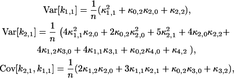
Next, each cumulant κ_i,j is replaced by its unbiased estimator k-statistic k_i,j (21) to construct the unbiased estimator of the factorial cumulant. In the case of κ_[2,1], we get , where represents the unbiased estimator of κ_[2,1]. The next task is to calculate the variance and covariance of k_i,j. We apply the tensor representation technique of Kaplan (22). The algorithm in Kaplan's article is implemented in Mathematica (Wolfram Research, Champaign, IL). For example, the variance and covariance of k_2,1 and k_1,1 are

(16)

where n is the total number of data points. To obtain this result, we take the large sample limit where n → ∞. The variance and covariance of k_i,j is now plugged into the variance of and results in the expression

(17)

Finally, the cumulants are transformed back to factorial cumulants by MathStatica,

(18)

Other variances of factorial cumulants are calculated in the same manner. We realize from this example that the resulting formulas are very long and cumbersome. However, all expressions are just simple polynomial and very easy to implement on computer. Here, for reference, we also list the variance of . The factorial cumulant κ_[1,1] and cumulant κ_1,1 are equal by definition. The unbiased estimator for is thus given by the corresponding k-statistics k_1,1. The variance Var[k_1,1] is given by the first line in Eq. 16. Again the cumulants κ_1,1, κ_0,2, κ_2,0, and κ_2,2 are transformed back into factorial cumulants. Evaluating the expression results in

(19)

Nonideal detector effect

Up to this point, the theory of factorial cumulants of the photon counts (Eq. 14) assumes that the photodetectors are ideal. Real detectors are never ideal and this needs to be taken into account in the theoretical description of photon count statistics. Particularly, dead-time and afterpulsing cause significant changes in the photon count statistics of PCH (18,19). An afterpulse is a fake pulse after the detection of a real photon count. Dead-time describes a period of time after the registration of a photon in which the detector is unable to generate photon signals. The dead-time of nonparalyzable detectors, such as an actively quenched avalanche photodiode (APD), is unaffected by photons reaching the detector during the dead-time. A detailed description of these nonideal effects on fluorescent fluctuation experiments, especially PCH analysis, can be found elsewhere (18,19). Here we discuss the effect of nonideal detectors on the factorial cumulants of the photon counts. In the following, primed quantities are used to represent physical quantities measured with a nonideal detector.

The factorial-moment-generating function (23) is an important theoretical tool for treating nonideal photodetector effects of factorial cumulant. It is based on the probability-generating function (23), which for a bivariate distribution P(k_A,k_B) is defined as

(20)

The factorial-moment-generating function is given by

(21)

When is expanded in a Taylor series, the coefficient of the u^mvⁿ/m!n! term describes the factorial moment μ_[m,n] (23).

Now let us first treat the effect of afterpulses, which has an analytical solution. Assume that after detecting a real count, there is a probability of P_Q, (Q = A, B), to observe a fake count. In addition, we postulate that different afterpulses are statistically independent from each other. Now suppose there are k_Q real counts detected in channel Q. The output counts k′_Q of the detector include afterpulses. We define a set of binary random variables (i = 1, …, k_Q) with a probability distribution

(22)

The definition of an afterpulse event leads to the following relation between k_Q and k′_Q,

(23)

The probability-generating function of (k′_A,k′_B) is given by

(24)

where P′ (k′_A,k′_B) is the probability distribution of afterpulse-influenced photon counts. With the help of a conditional probability distribution, we can relate P′ (k′_A,k′_B) to the distribution of real photon counts P (k_A,k_B),

(25)

The conditional distribution can be written as the product of afterpulse probabilities

(26)

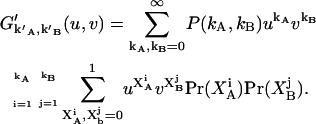
since different afterpulses are statistically independent from each other. Thus is given by

(27)

Notice that we plugged Eq. 23 into the exponent of u and v. Carrying out the products and the second summation results in

(28)

where is the probability-generating function for an ideal detector. Once the probability-generating function is known, the factorial-moment-generating function in the presence of afterpulsing is readily derived,

(29)

Taking derivative on both sides of the above equation, we obtain the relation between the afterpulse-influenced factorial moments and the ideal factorial moments. Since factorial cumulants can be expressed in terms of factorial moments, we established a relationship between the afterpulse-influenced factorial cumulant and the ideal factorial cumulant. The above algorithm is programmed in Mathematica and provides a convenient method to express the afterpulse-influenced factorial cumulant in terms of ideal factorial cumulants. A few simple cases are listed below,

(30)

To calculate the dead-time effect on factorial cumulants, we also consider the factorial-moment-generating function. We define the dead-time parameter as , where is the dead-time of the detector in channel Q and T is the sampling time. We only consider the case where δ_Q(T) is a small parameter. In this case the dead-time influenced probability-distribution function of photon counts can be expanded in a Taylor series of the dead-time parameters (19). We explicitly consider the first-order expansion,

(31)

The dead-time affected factorial moment generating function is

(32)

Plugging Eq. 31 into Eq. 32 and carrying out the summation, we obtain

(33)

Expanding both sides of the above equation in a Taylor series and comparing the coefficients of u and v, we obtain a relation between dead-time influenced factorial moments and ideal factorial moments. As was done in the case of the afterpulse effect, the factorial moments are used to express the dead-time influenced factorial cumulant in terms of ideal factorial cumulants. A few examples are listed below,

(34)

Higher-order expansions can be performed in a similar way and allow us to express the dead-time influenced moments in terms of ideal moments, but the results becomes more cumbersome and a simple analytical expression like Eq. 33 is not available. We explicitly treated the expansion up to the second-order and used it to correct for dead-time effects in the experimental data. Note that the derivation of the dead-time corrected cumulants is approximate. The maximum number of photon counts k_MAX received during the sampling time T by a nonparalyzable detector with dead-time τ^† is k_MAX = T/τ^†, but the theory sums photon counts from 0 to infinity. We have found that this approach describes fluorescence fluctuation data with 〈k〉δ ≤ 0.1, which translates into an intensity of 2 × 10⁶ cps for a dead-time of 50 ns (19,24).

MATERIALS AND METHODS

The instrument for the two-color fluorescence fluctuation experiments consists of a Zeiss Axiovert 200 microscope (Thornwood, NY) and a mode-locked Ti:Sapphire laser (Tsunami, Spectra-Physics, Mountain View, CA) pumped by an intracavity-doubled Nd:YVO4 laser (Millennia Vs, Spectra-Physics). A 63× Plan-Apochromat oil immersion objective (NA = 1.4) is used to focus the laser and collect the fluorescence. The light passes through an optical filter and is split into two channels. Photons counts are detected with an avalanche photodiode (APD) (SPCM-AQ-14, Perkin-Elmer, Dumberry, Québec). The output of the APD, which produces TTL pulses, was directly connected to a two-channel data acquisition card (FLEX02, Correlator.com, Bridgewater, NJ). The recorded photon counts were stored and later analyzed with programs written for IDL version 5.4 (Research Systems, Boulder, CO). A program written in Fortran with a nonlinear least-squares optimization routine from the Port Library (available at http://www.netlib.org) is used to fit the theoretical model to the experimental cumulants.

pEGFP-C1 and pEYFP-C1 plasmids were obtained from Clontech (Mountain View, CA). COS cells were obtained from ATCC (Manassas, VA) and maintained in 10% fetal bovine serum (Hyclone Laboratories, Logan, UT) and DMEM media. Cells were subcultured into an eight-well cover-glass slide (Naglenunc International, Rochester, NY) and then transiently transfected using Polyfect (Qiagen, Valencia, CA) according to manufacturer's instructions. Before conducting measurements, the grow media was removed and replaced with Leibovitz L15 (Invitrogen, Carlsbad, CA). All in vivo experiments are performed at an excitation wavelength of 960 nm, and a 515-nm dichroic mirror is used to separate the fluorescence into two detection channels.

In the dye experiments, Rhodamine 6G (Acros Organics, Morris Plains, NJ) and Rhodamine 110 (Molecular Probes, Eugene, OR) were dissolved in ethanol, and Alexa 488 (Molecular Probes) was dissolved in water. The stock solutions are diluted to appropriate concentrations for FFS experiments before each measurement. The dyes are excited at 780 nm. The Rhodamine 6G and Rhodamine 110 experiments employ a dichroic mirror with a transition wavelength of 544 nm and the Alexa 488 experiments use a 515-nm dichroic mirror.

We use the software MathStatica to derive formulas of factorial cumulants up to the eighth-order. The variance of the factorial cumulants is calculated up to the fourth-order by the technique of moments-of-moments with programs written in Mathematica. These formulas are implemented into an analysis program written in IDL (RSI, Boulder, CO) to calculate the experimental factorial cumulants and their errors.

We rebin the data to determine the factorial cumulants for different sampling times. The procedure is performed as follows: The recorded sequence of photon counts is fed into software to calculate the experimental factorial cumulants of photon counts of sampling time T. To get cumulant for a sampling or binning time of 2T, we add neighboring photon counts together to get a new sequence of photon counts with binning time 2T. We apply the same software algorithm on the rebinned data to get the cumulants for a binning time of 2T. This process is repeated to calculate the cumulants for binning times of specific integer multiples of T. By rebinning we calculate the factorial cumulants over sampling times that cover three orders of magnitude.

We fit the experimentally determined factorial cumulants to theoretical cumulants κ_[r,s] determined by Eq. 14 with a nonlinear least-squares fitting program. The reduced χ² of the fit is given by

(35)

The value of K is the total number of cumulants used in the fit and p is the number of free fitting parameters of the model.

RESULTS AND DISCUSSION

Single dye experiment

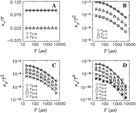
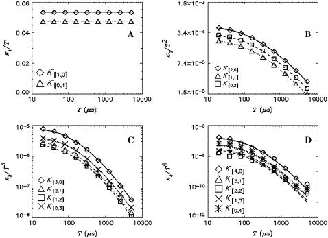
To test the dual-color TIFCA theory we perform experiments on simple fluorescent dye solutions. Each species is characterized by four parameters, its molecular brightness in each channel (λ_A and λ_B), the diffusion time τ_d, and the average occupation number N in V_PSF. For simplicity, we define the order of a bivariate cumulant by the sum of its indices. For example, the factorial cumulant κ_[i,j] is of (i + j)^th order. We fit cumulants with order smaller or equal to four simultaneously. Fig. 1 shows these cumulants as a function of binning time for Rhodamine 6G. The data was taken with a sampling time of 20 μs and a total measurement time of 130 s. The reduced χ² of the fit is 0.85 with a recovered brightness of λ_A = 34,000 cpsm, λ_B = 9600 cpsm, a diffusion time of τ_d = 44 μs, and an occupation number of N = 2.7.

FIGURE 1.

Dual-color cumulant analysis of a Rhodamine 6G solution. The data were taken with a sampling time of 20 μs and a total acquisition time of 130 s. Each cumulant is divided by T^r, where r = i + j is the order of the cumulant. The cumulants with the same order are plotted in the same panel. The best fit to a single species model is shown as lines. The fit determined λ_A = 34,000 cpsm and λ_B = 9600 cpsm, a diffusion time of τ_d = 44 μs, and an occupation number of N = 2.7 with a reduced χ² value of 0.85.

We now investigate the variance of the factorial cumulants as a function of binning time. The relative error of the factorial cumulant is given by and characterizes the noise/signal ratio. The experimental variance of is determined by the moments-of-moments method from the experimental factorial cumulants . We previously divided a long data set into shorter segments to directly calculate the measurement-to-measurement uncertainty of single-channel TIFCA and found that the moments-of-moments technique accurately reflects the experimental uncertainty of cumulants with order >1 (14). We verified using the same approach that the experimental uncertainty of cross cumulants is determined by the moments-of-moments technique (data not shown). We investigated the binning-time behavior of in the single-color case and found that initially decreases as a function of sampling time, but increases for long sampling times, which results in a minimum at some intermediate sampling time. This effect has been described in detail (14). 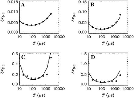It is interesting to explore the behavior of for the bivariate case. In Fig. 2 we plotted the relative errors of the first few important cross cumulants , , , and . Not surprisingly, all relative errors have minima with respect to the binning time. In other words, rebinning allows us to maximize the signal/noise ratio of factorial cumulants, just as in the single-color case. There is some small deviation in and between theory and experiments at very short and very long sampling times. This is caused by the large error in determining . Note that the deviation occurs where theory predicts a noise/signal ratio of ∼1, which indicates a large uncertainty in the experimental cumulant itself and leads to scattering of around the theoretical value. We also notice that the signal/noise ratio of cumulants decreases rapidly with its order. For example, the relative error of the cumulants in Fig. 2 increases by approximately one order-of-magnitude for each increase in order. Thus, this particular data set only contains statistically significant cumulants up to fourth-order.

FIGURE 2.

The relative error of factorial cumulants determined by the moments-of-moments analysis as a function of binning time. The diamonds represent the relative error calculated from the experimental data. We also calculated theoretical cumulants from the fit parameters and determine the relative error using the moments-of-moments variance (solid lines). The data were taken with a sampling time of 10 μs and a total data acquisition time of 130 s.

The moments-of-moments technique assumes statistically independent variables and ignores correlations between data points. The photon counts, however, are correlated with each other. We have discussed the effect of correlations on the variance of factorial cumulants (14). We concluded that the moments-of-moments technique is suitable to calculate the variance of the higher-order cumulants, but correction must be applied for the first-order. Because the order of all cross cumulants is larger than one, correlation effects can be safely ignored, which was confirmed by comparing with experimentally determined variances as discussed above.

Nonideal detector effects

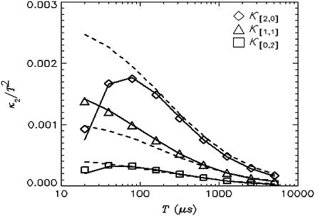
Nonideal detector effects can pronouncedly affect data analysis of fluorescence fluctuation experiments. We now consider their influence on cumulant analysis. The normalized second-order factorial cumulants (with i + j = 2) are plotted in Fig. 3 as a function of sampling time T for a concentrated Alexa 488 sample. The dashed line is a fit to the ideal model, which neglects nonideal detector effect. In this case, the quantity (with i + j = 2) should decay monotonically since it is proportional to the normalized binning function B₂/T², which we have shown to be a monotonically decreasing function (14). The ideal model fails to describe the data. This is especially noticeable for short sampling times T, where the dead-time parameter δ = τ^†/T is large and the dead-time effect is strong. The solid line in Fig. 3 shows the theoretical fit to the cumulants while taking nonideal detector effects into account and demonstrates that the corrections successfully model the data. Another interesting feature is that the cross-cumulant is much less influenced by nonideal detector effects than the univariate cumulant and . This is explained by looking at Eq. 34. The dead-time effect will always decrease the value of the univariate cumulants. In the short sampling time-limit T ≪ τ_d, the cumulant κ_[r,s] is proportional to T^r+s (14). The first-order correction to and thus scales as T². However, the correction to is proportional to T³ and the sign of the correction term can be positive or negative. So, for short sampling times (T → 0), the correction to is much smaller than that to and . When the sampling time is large, the dead-time parameter is small and the correction is small for both univariate and cross cumulants. Similar arguments apply to higher-order cumulants.

FIGURE 3.

The dead-time effect on the second factorial cumulant. A concentrated Alexa 488 solution was measured with a sampling time of 10 μs for 60 s. The average intensity measured is 817 kHz in channel A and 324 kHz in Channel B. The normalized second-order factorial cumulants (with i + j = 2) are plotted as a function of sampling time T. The dashed lines represent a fit to the data with the ideal model. Without dead-time effects, κ_[i,j]/T² should decay monotonically. The dead-time strongly influences the cumulant in the short sampling time limit, making the experimental cumulants smaller than the ideal ones. The fit to the nonideal model is shown as solid lines.

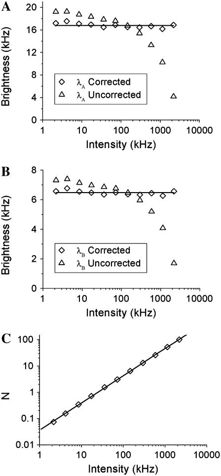
The factorial cumulants are used to determine the molecular brightness. Brightness is a molecular property, which has to be independent of the concentration of the fluorophore. Nonideal detector effects, however, destroy this independency (18,19). We perform a dilution experiment on an Alexa 488 sample to check the concentration-dependence of the brightness in dual-color cumulant analysis. A concentrated Alexa 488 sample was successively diluted by factors of two and measured after each dilution step for 60 s with a sampling time of 20 μs. Fits of the data to the ideal model recovered a biased brightness shown as triangles in Fig. 4 that depends on the intensity and therefore on the concentration of the sample. Next we fit the factorial cumulants of all data globally to the nonideal model by linking the γ₃ and γ₄ parameters across all data sets while all other parameters are free to vary. The γ₃ and γ₄ parameter reflect the shape of the PSF and have to be the same for all data sets. From the fit, it is determined that γ₃ = 0.242 and γ₄ = 0.196. The brightness in each channel is plotted as diamonds in Fig. 4, A and B. Comparison of the brightness values recovered from the fit to the ideal and nonideal model shows that the brightness is concentration-independent only by accounting for dead-time and afterpulsing. Afterpulsing mainly influences data analysis when the intensity is low and it increases the brightness value, while the effect of dead-time is most dramatic at high intensities and decreases the brightness as previously discussed (19,24). Fig. 4 C graphs the number of molecules determined from a fit to the nonideal model as a function of the fluorescence intensity. A straight line describes the data, as expected, because the intensity is proportional to the concentration. Neglecting nonideal detector effects leads to a deviation of the data from a straight line (data not shown). This example serves to highlight the importance of accounting for nonideal detector effects to recover unbiased brightness and concentration values. The intensity of the photon counts in this experiment runs from one thousand to two million counts per second, which means the algorithm used for correcting nonideal effects covers the useful intensity range of photon-counting experiments.

FIGURE 4.

Alexa 488 was diluted repeatedly in water by factors of two and the cumulants of each sample were fit using the ideal and nonideal model. The sampling time is 20 μs and the data acquisition time is 60 s. In panel A (B) the molecular brightness of channel A (B) is plotted. The uncorrected brightness recovered by the ideal model, plotted as triangles, depends on the concentration of the sample. The brightness decreases at higher concentration due to the influence of dead-time and increases at lower concentrations due to afterpulses. The nonideal model is used to correct for nonideal detector effects and recovers a concentration-independent brightness, which is plotted as diamonds. The lines represent the average value measured in each channel. (C) The number of molecules (diamonds) recovered from the fit to the nonideal model is plotted as a function of intensity. The graph is well described by a fit to a straight line as expected. The dead-time and afterpulse parameters of our APDs have been determined previously (19) and are fixed during the fit of the data. Their values for both instruments are: Instrument 1, ,, P_AA = 0.002, and P_AB = 0.003; and Instrument 2: ,, P_AA = 0.007, and P_AB = 0.0046.

Binary dye mixture

Resolving a binary mixture in dual channel experiments requires the determination of eight parameters: the molecular brightnesses (λ_Ai, λ_Bi), the diffusion time τ_di, and the number of molecules N_i of each species i. Stock solutions of Rhodamine 6G and Rhodamine 110 are mixed together and measured for 130 s. Fig. 5 shows a two-species fit to the factorial cumulants up to fourth-order. The reduced χ² is 0.93, which indicates good agreement between model and experimental data. A fit to a single species model fails to describe the data (χ² = 478). The parameters recovered from the two-species fit are: λ_A1 = 34,000 cpsm, λ_B1 = 9300 cpsm, τ_d1 = 48 μs, and N₁ = 1.07, which nicely agree with the values recovered from an independent measurement of a Rhodamine 6G solution (see Fig. 1). For the second species we determined λ_A2 = 11,000 cpsm, λ_B2 = 24,000 cpsm, τ_d2 = 49 μs, and N₂ = 1.58. These parameters agree well with an independent measurement of a Rhodamine 110 solution, which resulted in λ_A = 11,000 cpsm, λ_B = 26,000 cpsm, and τ_d = 47 μs (data not shown).

FIGURE 5.

A binary mixture of Rhodamine 6G and Rhodamine 110 resolved by dual-color TIFCA. A 544-nm dichroic mirror was used to separate the emission into two detection channels. The data was taken with a sampling time of 20 μs for 130 s. Fitting the cumulants up to fourth-order to a single-species model (data not shown) returns a reduced χ² value of 478. A two-species model fits the experimental cumulants within error (χ² of 0.93). The parameters recovered from the two-species fit are: λ_A1 = 34,000 cpsm, λ_B1 = 9300 cpsm, τ_d1 = 48 μs, and N₁ = 1.07 for Rhodamine 6G and λ_A2 = 11,000 cpsm, λ_B2 = 24,000 cpsm, τ_d2 = 49 μs, and N₂ = 1.58 for Rhodamine 110.

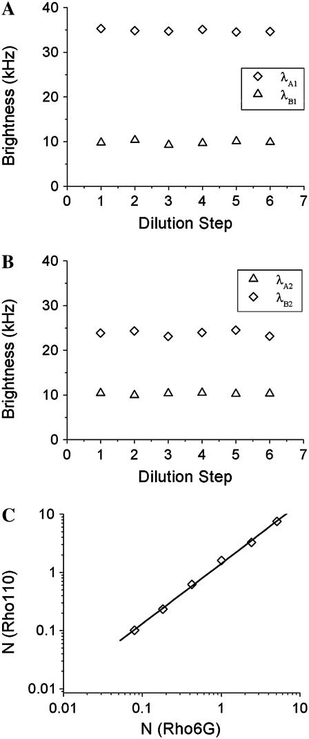
Next, we perform a dilution experiment of a binary dye mixture to judge the robustness of the technique. The concentrated stock solutions of Rhodamine 6G and Rhodamine 110 were mixed together and diluted successively. Each data set is fit to a two-species model. The reduced χ² of the fits varied between 0.75 and 1.7. The fitted molecular brightness of Rhodamine 6G and Rhodamine 110 is shown in Fig. 6, A and B. The brightness is concentration-independent as expected. The diffusion time recovered for Rhodamine 6G varied from 44 μs to 48 μs with an average of 45 μs, whereas the diffusion time of Rhodamine 110 varied from 48 μs to 52 μs with an average of 50 μs. The average diffusion time of the two species agrees within 5% with the values determined from measurements of the individual dye solutions. Fitting the number of molecules of both species shown in Fig. 6 C to a straight line yields a slope of 1.45, which characterizes the concentration ratio of the two fluorophores in solution.

FIGURE 6.

Dual-color TIFCA analysis of a binary dye mixture of Rhodamine 6G and Rhodamine 110. The mixture was repeatedly diluted and measured for 130 s after each dilution. Each data set is fit to a two-species model. The brightness recovered from the fit is plotted in panels A and B for Rhodamine 6G and Rhodamine 110, respectively. The brightness in channel A is shown as diamonds, while the brightness in channel B is graphed as triangles. The number of molecules is plotted in panel C. The numbers of molecules of both species are linearly related as expected, because the concentration ratio remains constant during dilution. A fit of the data to a straight line recovers a slope of 1.45, which reflects the concentration ratio of the dyes in the mixtures.

EGFP and EYFP in living cell

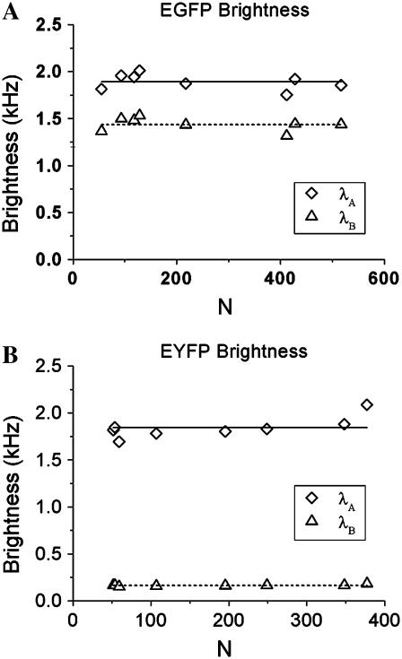
FFS is a powerful tool for studying protein function in living cells. Brightness can be used to probe protein association and dissociation in cells (25). Here we demonstrate that dual-color TIFCA is sufficiently robust to be applied in living cells. The brightness of fluorescent proteins, such as EGFP and EYFP, in living cells is low. In addition, the concentration of fluorophores is often quite high. To demonstrate the feasibility of dual-color TIFCA in this challenging environment we first show that the brightness of each FP is concentration-independent. We transiently transfect COS cells with EGFP or EYFP, perform FFS measurements, and fit the cumulants to a single-species model. The brightness of Channel A (diamonds) and B (triangles) of EGFP and EYFP is plotted in Fig. 7, A and B. Their brightnesses are concentration-independent as expected. Note that without correcting for nonideal detector effects, the brightness of each channel would display a concentration-dependent behavior similar to that shown for Alexa 488 in Fig. 4.

FIGURE 7.

The brightness values of EGFP and EYFP as obtained from dual-color TIFCA analysis of cellular measurements is shown in panels A and B. Nonideal detector effects are taken into account during the analysis. The brightness in channel A is graphed as diamonds and that of channel B is shown as triangles. Each data point represents the measurement of a different cell. The sampling and data acquisition time for each measurement was 50 μs and 120 s. Since EGFP and EYFP are monomeric in cells, their brightness remains constant as the concentration increases. The solid and dotted lines indicate the average brightness measured in each channel.

EGFP and EYFP: resolvability study

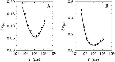
It is known that for two-channel FFS experiment, each species is characterized by four parameters λ_A, λ_B, τ_d, and N. The diffusion time τ_d is determined from the shape of the time-dependent cumulant function κ_[m,n](T). Therefore three cumulants are needed to identify the remaining three parameters of each species. For example, a binary mixture requires the knowledge of six cumulants. If the experimental data only contain statistically significant cumulants up to second-order, only five cumulants are known, which is insufficient for resolving two species. However, if the third-order cumulants are statistically significant, a total of nine measurable cumulants are present: κ_[1,0], κ_[0,1], κ_[2,0], κ_[1,1], κ_[0,2], κ_[3,0], κ_[2,1], κ_[1,2], and κ_[0,3], which opens up the possibility to directly resolve two species in a cell with a single measurement. Fig. 8 shows the relative error of and of EGFP measured in a living cell. A relative error <1 indicates that the cumulant is statistically significant. For this data, all third-order cumulants are statistically significant. Since the data contain nine significant cumulants, it is possible to directly resolve species in the living cell. Again, we find that rebinning helps to optimize the signal/noise ratio, which increases the sensitivity of our data analysis.

FIGURE 8.

The relative error of third-order cumulants measured for EGFP in a living cell. The data is taken with sampling time of 50 μs and a total acquisition time of 330 s. The relative errors of (A) and (B) are plotted as a function of binning time. The symbols are experimental data and the solid lines represent the theoretical curve calculated from the parameters recovered by the fit.

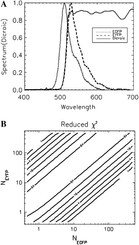
The error analysis of cumulants allows experimentalists to predict whether species can be resolved based on measured properties of fluorophores. To illustrate this point, we apply a similar strategy as used in Müller et al. (26). Theoretical factorial cumulants of two species are calculated with Eq. 14. The variances of the cumulants are calculated using the moments-of-moments technique. A fit of the two-species cumulants by a single-species model will result in a misfit, which gives rise to systematic residuals. The magnitude of these residuals tells us whether it is feasible to distinguish the binary mixture from a single species. The reduced χ² is a convenient measure of this systematic deviation induced by the forced fit to a single species. A reduced χ² value ≤1 indicates that the data is not sufficient to resolve the species, while a χ² >1 indicates that more than one species is present.

We now study the concentration-dependence of the χ² describing the misfit for an EGFP/EYFP mixture. In Fig. 9 A, the emission spectra of these two proteins are plotted together with the transmission curve of the 515-nm dichroic mirror used in the experiments. The strong spectral overlap poses a challenging problem for resolving these two proteins by FFS (17). We took the average brightness and diffusion time of EGFP and EYFP measured earlier (see Fig. 7) and plugged them into a two-species cumulant model, while the number of molecules of EGFP and EYFP is varied systematically. Cumulants and their variances are calculated assuming a sampling time of 50 μs and a data acquisition time of 300 s. The cumulants are fit to a single-species model and the χ² value describing the misfit is recorded. A contour plot of the χ² value versus the number of molecules best illustrates the concentration-dependence of the resolvability. To our surprise, the misfit χ² value depends essentially only on the concentration ratio of the two fluorophores, but is largely independent of the overall concentration. This is drastically different from a similar single-color (26) and dual-color PCH study (data not shown), where the optimal concentration for resolving species is typically on the order of one molecule in the observation volume. This constitutes a clear advantage of dual-color TIFCA for cellular application, where the concentration of fluorophores is usually very high. Note that this simulation neglects some of the experimental complications encountered in cells. Autofluorescence adds a background signal that limits the resolvability at low concentrations, while photo detectors introduce complexity that cannot be described by our simple model when the intensity is extremely high.

FIGURE 9.

Resolvability study of EGFP and EYFP in living cell. (A) The emission spectra of EGFP and EYFP are plotted together with the transmission curve of the 515-nm dichroic mirror used in the experiments. (B) The contour plot shows the reduced χ² value when fitting a single-species model to the theoretical cumulants of the two-species model. See text for a description of the method. The experimentally determined brightness and diffusion time of EGFP and EYFP are used as inputs for calculating the theoretical cumulants. The concentration of EGFP and EYFP are varied logarithmically. The sampling time for this simulation is 50 μs and the data acquisition time is 300 s. The χ² value depends mainly on the ratio between the concentrations of the two species and only weakly on the absolute concentrations.

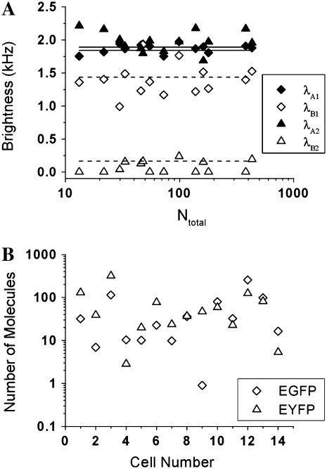
Resolving EGFP/EYFP binary mixtures in living cells

To test the robustness of dual-color TIFCA for resolving a binary mixture of fluorescent proteins, we cotransfect COS cells with EGFP and EYFP. Each cell is measured for 5 min with a sampling time of 50 μs. The single-species fit to these data depends on the cotransfection ratio of the two proteins and returns reduced χ²values that range from 10 to 100, which indicate that we are dealing with mixtures. Different cells have different protein concentrations and cotransfection ratios. However, because brightness is a molecular property, it should not change with concentration and must be independent from the cell measured. Fig. 10 A shows the molecular brightness in each channel recovered from a two-species model as a function of the total number of EGFP and EYFP molecules. The lines represent the average brightness of EGFP and EYFP reported in Fig. 7. It is clear that the parameters recovered from the fit closely resemble the EGFP and EYFP brightness values from the single-species experiments. Fig. 10 B shows the number of molecules of EGFP and EYFP for each measured cell. The concentration of EGFP and EYFP varies widely from cell to cell as expected for a transient transfection. For our experimental conditions one molecule corresponds to a concentration of 4.5 nM. Thus, we are able to resolve the two fluorescent proteins from nanomolar to micromolar concentrations. Dual-color PCH analysis is applied to some of the data, and fits to a single-species model returned reduced χ² values close to one, which indicates that PCH is unable to resolve the mixture.

FIGURE 10.

Mixture of EGFP and EYFP resolved by dual-color TIFCA. COS cells are transiently cotransfected with EGFP and EYFP before measurements. (A) The brightness of species 1 (diamonds) and species 2 (triangles) in channel A (solid symbol) and B (open symbol) is plotted as a function of the total number of molecules. The lines are average value of EGFP and EYFP as measured in Fig. 7. The comparison shows that species 1 corresponds to EGFP, while species 2 is EYFP. The sampling time for each measurement is 50 μs and the data acquisition time is 300 s. (B) The number of molecules of EGFP (diamonds) and EYFP (triangles) is plotted for each measured cell.

CONCLUSION

We developed the theory of dual-color time-integrated fluorescence cumulant analysis to extract information from bivariate factorial cumulants of the photon counts. This theory is in contrast to PCH since it is exact for all sampling times. The error analysis of cumulants allows experimentalists to predict in advance whether the experimental conditions are sufficient for resolving species and helps in identifying optimal experimental conditions. The dead-time and afterpulsing effect of the photo detector are also taken into account in the theory, which allows one to recover consistent parameter over a concentration range of approximately three orders of magnitude. The theory is tested with simple dye experiments to determine the brightness, the number of molecules, and the diffusion time of fluorophores from a single measurement. We recover brightness values of fluorescent proteins in living cells to demonstrate that the technique is sufficiently robust for cellular applications. Finally, we demonstrated the power of dual-color TIFCA by resolving binary mixture of EGFP and EYFP over a wide concentration range in living cells.

References

- 1.Denk, W., J. H. Strickler, and W. W. Webb. 1990. Two-photon laser scanning fluorescence microscopy. Science. 248:73–76. [DOI] [PubMed] [Google Scholar]
- 2.Rigler, R., U. Mets, J. Widengren, and P. Kask. 1993. Fluorescence correlation spectroscopy with high count rate and low background: analysis of translational diffusion. Eur. Biophys. J. 22:169–175. [Google Scholar]
- 3.Magde, D., E. L. Elson, and W. W. Webb. 1974. Fluorescence correlation spectroscopy. II. An experimental realization. Biopolymers. 13:29–61. [DOI] [PubMed] [Google Scholar]
- 4.Chen, Y., J. D. Müller, P. T. So, and E. Gratton. 1999. The photon-counting histogram in fluorescence fluctuation spectroscopy. Biophys. J. 77:553–567. [DOI] [PMC free article] [PubMed] [Google Scholar]
- 5.Kask, P., K. Palo, D. Ullmann, and K. Gall. 1999. Fluorescence-intensity distribution analysis and its application in biomolecular detection technology. Proc. Natl. Acad. Sci. USA. 96:13756–13761. [DOI] [PMC free article] [PubMed] [Google Scholar]
- 6.Palo, K., U. Mets, S. Jager, P. Kask, and K. Gall. 2000. Fluorescence intensity multiple distributions analysis: concurrent determination of diffusion times and molecular brightness. Biophys. J. 79:2858–2866. [DOI] [PMC free article] [PubMed] [Google Scholar]
- 7.Laurence, T. A., N. A. Kapanidis, X. D. Kong, S. Chemla, and S. Weiss. 2004. Photon arrival-time interval distribution (PAID): a novel tool for analyzing molecular interactions. J. Phys. Chem. B. 108:3051–3067. [Google Scholar]
- 8.Gopich, I. V., and A. Szabo. 2005. Photon counting histograms for diffusing fluorophores. J. Phys. Chem. B. 109:17683–17688. [DOI] [PubMed] [Google Scholar]
- 9.Qian, H., and E. L. Elson. 1990. On the analysis of high order moments of fluorescence fluctuations. Biophys. J. 57:375–380. [DOI] [PMC free article] [PubMed] [Google Scholar]
- 10.Qian, H. 1990. On the statistics of fluorescence correlation spectroscopy. Biophys. Chem. 38:49–57. [DOI] [PubMed] [Google Scholar]
- 11.Palmer, A. G., and N. L. Thompson. 1987. Molecular aggregation characterized by high order autocorrelation in fluorescence correlation spectroscopy. Biophys. J. 52:257–270. [DOI] [PMC free article] [PubMed] [Google Scholar]
- 12.Palmer, A. G., and N. L. Thompson. 1989. High-order fluorescence fluctuation analysis of model protein clusters. Proc. Natl. Acad. Sci. USA. 86:6148–6152. [DOI] [PMC free article] [PubMed] [Google Scholar]
- 13.Müller, J. D. 2004. Cumulant analysis in fluorescence fluctuation spectroscopy. Biophys. J. 86:3981–3992. [DOI] [PMC free article] [PubMed] [Google Scholar]
- 14.Wu, B., and J. D. Müller. 2005. Time-integrated fluorescence cumulant analysis in fluorescence fluctuation spectroscopy. Biophys. J. 89:2721–2735. [DOI] [PMC free article] [PubMed] [Google Scholar]
- 15.Schwille, P., F. J. Meyer-Almes, and R. Rigler. 1997. Dual-color fluorescence cross-correlation spectroscopy for multicomponent diffusional analysis in solution. Biophys. J. 72:1878–1886. [DOI] [PMC free article] [PubMed] [Google Scholar]
- 16.Kask, P., K. Palo, N. Fay, L. Brand, U. Mets, D. Ullmann, J. Jungmann, J. Pschorr, and K. Gall. 2000. Two-dimensional fluorescence intensity distribution analysis: theory and applications. Biophys. J. 78:1703–1713. [DOI] [PMC free article] [PubMed] [Google Scholar]
- 17.Chen, Y., M. Tekmen, L. Hillesheim, J. Skinner, B. Wu, and J. D. Muller. 2005. Dual-color photon-counting histogram. Biophys. J. 88:2177–2192. [DOI] [PMC free article] [PubMed] [Google Scholar]
- 18.Hillesheim, L. N., and J. D. Muller. 2003. The photon counting histogram in fluorescence fluctuation spectroscopy with nonideal photodetectors. Biophys. J. 85:1948–1958. [DOI] [PMC free article] [PubMed] [Google Scholar]
- 19.Hillesheim, L. N., and J. D. Müller. 2005. The dual-color photon counting histogram with nonideal photodetectors. Biophys. J. 89:3491–3507. [DOI] [PMC free article] [PubMed] [Google Scholar]
- 20.Mandel, L. 1958. Fluctuations of photon beams and their correlations. Proc. Phys. Soc. 72:1037–1048. [Google Scholar]
- 21.Kendall, M. G., and A. Stuart. 1977. Chapter 12. In The Advanced Theory of Statistics, Vol. 1. MacMillan, New York.
- 22.Kaplan, E. L. 1952. Tensor notation and the sampling cumulants of k-statistics. Biometrika. 39:319–323. [Google Scholar]
- 23.Saleh, B. 1978. Photoelectron Statistics. Springer-Verlag, New York.
- 24.Sanchez-Andres, A., Y. Chen, and J. D. Muller. 2005. Molecular brightness determined from a generalized form of Mandel's Q-parameter. Biophys. J. 89:3531–3547. [DOI] [PMC free article] [PubMed] [Google Scholar]
- 25.Chen, Y., L. N. Wei, and J. D. Müller. 2003. Probing protein oligomerization in living cells with fluorescence fluctuation spectroscopy. Proc. Natl. Acad. Sci. USA. 100:15492–15497. [DOI] [PMC free article] [PubMed] [Google Scholar]
- 26.Müller, J. D., Y. Chen, and E. Gratton. 2000. Resolving heterogeneity on the single molecular level with the photon-counting histogram. Biophys. J. 78:474–486. [DOI] [PMC free article] [PubMed] [Google Scholar]