Comparative visualization for comprehensive two-dimensional gas chromatography

Abstract

This paper investigates methods for comparing datasets produced by comprehensive two-dimensional gas chromatography (GC × GC). Chemical comparisons are useful for process monitoring, sample classification or identification, correlative determinations, and other×important tasks. GC × GC is a powerful new technology for chemical analysis, but methods for comparative visualization must address challenges posed by GC × GC data: inconsistency and complexity. The approach extends conventional techniques for image comparison by utilizing specific characteristics of GC × GC data and developing new methods for comparative visualization and analysis. The paper describes techniques that register (or align) GC × GC datasets to remove retention-time variations; normalize intensities to remove sample amount variations; compute differences in local regions to remove slight misregistrations and differences in peak shapes; employ color (hue), intensity, and saturation to simultaneously visualize differences and values; and use tools for masking, three-dimensional visualization, and tabular presentation with controls for graphical highlights to significantly improve comparative analysis of GC × GC datasets. Experimental results indicate that the comparative methods preserve chemical information and support qualitative and quantitative analyses.

1. Introduction

This paper investigates methods for comparing datasets produced by comprehensive two-dimensional gas chromatography (GC × GC). Chemical comparisons are useful for process monitoring, sample classification or identification, correlative determinations, and other important tasks. GC × GC [1] is a powerful new chemical separation technology that provides significant advantages over traditional GC: an order-of-magnitude increase in chemical separation capacity, higher-dimensional chemical ordering, and a significant increase in signal-to-noise ratio. GC × GC has important potential uses for comparative chemical analysis, for example:

• comparing manufactured products with standards for quality control [2];

• monitoring actual or potential pollution sites for environmental changes [3];

• surveying crime scenes for chemical “fingerprints” [4]; and

• assaying classes of tissue samples for biomarker discovery [5].

The lack of software for GC × GC data and information processing has been a significant×impediment to the adoption of GC × GC for routine applications, but that problem is beginning to be addressed by recent availability of software specifically for GC × GC [6].

This paper addresses two challenges for computer-based comparative visualization and analysis of GC × GC datasets: data inconsistency and complexity. First, GC × GC datasets exhibit inconsistencies in sample amounts, peak retention times, and peak shapes that are caused by uncontrolled chromatographic variations and which are not related chemical differences in the samples. If these incidental variations are not removed from the comparison, they can confound and obscure actual chemical differences. Second, even if incidental inconsistencies are removed, the chemical comparisons typically are complex and difficult to visualize and report. In particular, GC × GC data may contain thousands of peaks in complex multi-dimensional patterns related to chemical structure. Moreover, different comparative aspects, such as absolute differences or relative differences, may be more or less important for different chemicals and for different applications. Presenting complex comparisons of complex data on a computer monitor or printed page is challenging.

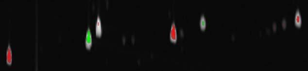
The approach in this paper is to extend conventional techniques for image comparison by utilizing specific characteristics of GC × GC data and developing new methods for comparative visualization and analysis. GC × GC data can be represented, visualized, and processed as an image, e.g., a[m, n] where a is the analyzed chromatogram with pixels indexed by first-column retention-time m (increasing left-to-right) and second-column retention-time n (increasing bottom-to-top). As in Fig. 1, each resolved compound produces a small two-dimensional peak with pixel values (or intensities) that are larger than the background values and can be visually distinguished through pseudo-color mapping of the pixel values. Then, two GC × GC datasets can be compared by simple techniques, such as side-by-side comparison or flicker (i.e., alternating) between images [7], or by digital image processing methods, such as creating a difference image (by subtraction) or addition image (by addition in different colors) [8-10]. The pixel values also can be interpreted as elevation, generating a three-dimensional surface which can be projected to two dimensions for visualization.

Fig. 1.

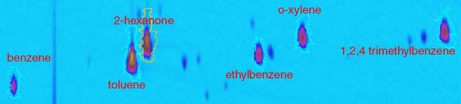
Analyzed chromatographic image for comparison.

The methods developed in Section 2 use GC × GC metadata, such as peak identifications and quantifications, to register (i.e., align) retention times between two data sets (correcting for incidental variations of retention times) and to normalize values between two data sets (correcting for incidental differences in sample amounts). Section 3 develops a new colorized difference method to visually emphasize the remaining differences and a new fuzzy difference method that can be used to suppress variations of peak shape in order to highlight differences in chemical composition. Section 4 describes an interactive peak comparison table that provides analysts with quantitative data and control of peak-oriented graphical overlays and an interactive environment for three-dimensional viewing that enables analysts to combine comparison methods using elevation. Section 5 examines issues for further research and development.

2. Data processing

This paper considers comparisons between two GC × GC images—the dataset currently selected for analysis, referred to as the analyzed image, is compared to another image, referred to as the reference image. Prior to comparison, each GC × GC image is processed separately to correct acquisition artifacts (e.g., background removal [11]) and to detect and quantify chemical peaks [6], steps that can be performed by GC × GC software in a few seconds. Then, two additional data processing steps— registration and normalization—are performed on the reference image to remove incidental differences with the analyzed image. Section 2.1 describes the process of registering the reference image with the analyzed image so that the retention times of peaks in the reference image align with the retention times of the corresponding peaks in the analyzed image. Section 2.2 describes value (or intensity) scaling to normalize the response (i.e., total peak intensity) for quantitative standard(s) in the reference image to the response for standard(s) in the analyzed image. These two steps are critical for suppressing incidental variations and emphasizing only real chemical differences.

2.1. Registration

Registration transforms the reference image so that when it is overlaid on the analyzed image, the retention times of the corresponding peaks are aligned. Registration consists of two steps: (1) determine a transformation of the reference image to remove differences in retention times and (2) resample the transformed reference image at the pixel locations of the analyzed image.

Various two-dimensional geometric transformations have been used for digital image processing [12]. Affine transformation has been shown to effectively remove retention variations related to chromatographic parameters [13]. The transformed two-dimensional retention times (x _t ,y _t) are computed from the reference image retention times (x _r ,y _r) as:

$$\left[\begin{array}{c}\hfill x_{\mathrm{t}}\hfill \\ \hfill y_{\mathrm{t}}\hfill \end{array}\right]=\left[\begin{array}{cc}\hfill a\hfill & \hfill b\hfill \\ \hfill c\hfill & \hfill d\hfill \end{array}\right]\left[\begin{array}{c}\hfill x_{\mathrm{r}}\hfill \\ \hfill y_{\mathrm{r}}\hfill \end{array}\right]+\left[\begin{array}{c}\hfill e\hfill \\ \hfill f\hfill \end{array}\right]$$ (1)

where a-f are the parameters of affine transformation.

The parameters of affine transformation can be fit to minimize the mean-square difference between the transformed retention times of a set of peaks in the reference image and the retention times of the corresponding peaks in the analyzed image. Only three pairs of non-colinear corresponding peaks are required to determine an affine transformation, but automated pattern matching can be used to establish many correspondences even for peaks whose chemical identity has not yet been established [14]. For GC × GC-MS, mass spectral matching can be used in conjunction with pattern matching [15] to establish peak correspondences. The task of identifying peaks by chemical names can be performed prior to comparative analysis (e.g., in the template used for pattern matching) or it can be performed after comparative analysis (e.g., on peaks that differ in the two samples).

Let B be the set of (at least three) corresponding peaks b_i, such that each peak is present in both the analyzed and reference images with retention times (x _a(b_i), y _a(b_i)) and (x _r(b_i), y _r(b_i)), respectively. Then, the parameters of the transformation are set to minimize:

$$E=\frac{1}{\mid B\mid }\sum _{b_i\in B}\sqrt{{(x_{\mathrm{a}}\left(b_i\right)-x_{\mathrm{t}}\left(b_i\right))}^2+{(y_{\mathrm{a}}\left(b_i\right)-y_{\mathrm{t}}\left(b_i\right))}^2}.$$ (2)

Registration could be made more precise by using locally adaptive transformations rather than a global transformation, but locally adaptive registration is more sensitive to errors.

One possible problem is that mismatched pairs of peaks can reduce the accuracy of the transformation. To avoid this, after the first transformation is computed from the set of all corresponding peaks, the peaks for which the transformed retention times differ most from the corresponding-peak retention times in the analyzed image are removed from the peak set B and the least-squares fit is recomputed on the remaining peaks. Observations suggest that removing the 25% of peak pairs with the largest differences effectively removes mismatched pairs. At least three non-colinear points must be retained in the peak set to uniquely determine the optimal affine transformation. Experimental results, presented in Section 3, indicate that this registration process accurately aligns even peak pairs which are not in the peak set B used to optimize the transformation.

The reference image is then transformed, interpolated, and resampled at the pixel locations of the analyzed image. Interpolating by convolution yields the transformed image t:

$$t[x_{\mathrm{t}},y_{\mathrm{t}}]=\sum _{m^{\prime },n^{\prime }}r[m^{\prime },n^{\prime }]f(x_{\mathrm{r}}-m^{\prime },y_{\mathrm{r}}-n^{\prime }),$$ (3)

where r is the reference image and f is the interpolation function. Bilinear interpolation is a simple, yet effective two-dimensional interpolator [16].

2.2. Normalization

For two runs (even from the same sample), slightly different sample amounts are introduced and so produce different responses. Differences in GC × GC images due to variable sample amounts must be corrected so that they are not mistaken as differences in concentrations.

GCxGC intensities are relatively linear with respect to amount, so normalization can be implemented by multiplicative scaling. The scale factor is set to equalize the response in the analyzed and reference images to one or more quantitative standards which are taken to have the same concentrations in both samples. For example, in analyzing chemical changes over time at the site an oil spill, Nelson et al. [17] used hopane for quantitative normalization because it is relatively persistent over the observation period.

At least one peak is required as a quantitative standard to normalize relative amounts. Given a set S with corresponding peak(s) b_i, where V _a(b_i) is the detected volume (total peak response) in the analyzed image and V _r(b_i) is the detected volume in the reference image, the normalization scale factor is computed as:

$$F=\frac{\sum _{b_i\in S}{V}_{\mathrm{a}}\left(b_i\right)}{\sum _{b_i\in S}{V}_{\mathrm{r}}\left(b_i\right)}.$$ (4)

Just as for registration, mismatched pairs of peaks can reduce the accuracy of normalization. The same method for avoiding registration errors can be used to avoid normalization errors. The scale factor is first computed for all quantitative standards. Then, the scale factor is applied to the individual volumes of the quantitative peaks in the reference image. The 25% of quantitative standards with the greatest difference magnitude between the scaled reference volume and the analyzed volume are removed from the set of quantitative standards and the scale factor is recomputed. Experimental results, presented in Section 3, indicate that this scaling allows direct qualitative and quantitative comparisons of corresponding peaks.

The scale factor is applied to each pixel of the transformed reference image:

$$s[m,n]=F\cdot t[m,n]$$ (5)

The transformed and scaled reference image s now can be compared to the analyzed image a.

3. Image-based comparison methods

This section illustrates several image-based comparison methods using two GC × GC datasets of calibration samples for the ASTM D5580 method [18] (provided by Zoex Corporation). Each calibration sample contained five chemicals, listed in Table 1, in differing amounts, to provide a range for calibration, and an internal standard, 2-hexanone. As shown in Table 1, toluene had the largest relative amount in the analyzed sample and ethylbenzene had the largest relative amount in the reference sample. Two chemicals (toluene and orthoxylene) were present in larger relative amounts in the analyzed sample than in the reference sample and three chemicals (benzene, ethylbenzene, and 1,2,4-trimethylbenzene) were present in smaller amounts in the analyzed sample than in the reference sample. The expected relative differences express the differences relative to the amounts and are computed as:

$$\text{Expected relative difference}\left(i\right)=\frac{A_{\mathrm{a}}\left(i\right)∕A_{\mathrm{a}}\left(s\right)-A_{\mathrm{r}}\left(i\right)∕A_{\mathrm{r}}\left(s\right)}{A_{\mathrm{a}}\left(i\right)∕A_{\mathrm{a}}\left(s\right)+A_{\mathrm{r}}\left(i\right)∕A_{\mathrm{r}}\left(s\right)}$$ (6)

where A _a(i) and A _r(i) are the amounts of chemical i in the analyzed and reference samples, respectively, and A _a(s) and A _r(s) are the amounts of the internal standard s in the analyzed and reference samples, respectively. The relative difference is bounded by -1.0 and 1.0. The observed relative differences and relative errors in Table 1 are discussed in Section 4.2. The subimage of the analyzed image used for visualization is shown in Fig. 1.For the visualization examples in this section, the images were registered using only toluene, 2-hexanone, and ethylbenzene and were normalized using the responses to 2-hexanone.

Table 1.

Calibration sample chemicals: relative amounts, expected relative differences, observed relative differences, and relative error

Chemical	Analyzed relative amount	Reference relative amount	Expected relative difference	Observed relative difference	Relative error (%)
Benzene	0.090	4.399	- 0.9599	- 0.9602	- 0.03
Toluene	13.500	0.879	0.8777	0.8761	- 0.17
Ethylbenzene	0.450	8.798	- 0.9027	- 0.9011	0.15
Orthoxylene	0.900	0.439	0.3444	0.3449	0.05
1,2,4-Trimethylbenzene	0.900	2.209	- 0.4211	- 0.4191	0.20

3.1. Grayscale difference

A popular method for comparing two images is to form a difference image by subtracting the individual pixel values of one image from the corresponding pixel values of the other image [8]. The comparison techniques developed in this paper extend the difference image method.

In these comparisons, the reference image is subtracted from the analyzed image, so a positive difference indicates that the analyzed image has a larger pixel value and a negative difference indicates that the reference image has a larger pixel value. The difference image can be displayed with a grayscale so that medium gray represents zero difference, brighter values represent positive differences, and darker values represent negative differences. The larger the magnitude of the difference, the closer the displayed pixel is to white or black. A logarithmic scale can be used to better highlight differences with smaller magnitudes, but the same scale factor is used for both positive and negative values.

The example grayscale difference image is shown in Fig. 2. Visually, the peaks for benzene (left edge), ethylbenzene (center), and 1,2,4-trimethylbenzene (right edge) are dark, indicating the analyzed sample has smaller amounts than the reference sample (relative to 2-hexanone). Note that the peaks which were not used for registration, benzene and 1,2,4-trimethylbenzene, are aligned well, even though they are on the periphery of the subregion. The magnitudes of the differences are discernible: the peak for ethylbenzene is darker than the peak for 1,2,4-trimethylbenzene, illustrating that the difference in amounts between the analyzed and reference image is greater for ethylbenzene than for 1,2,4-trimethylbenzene. The peaks for toluene and orthoxylene are mostly bright, indicating that the analyzed sample has larger relative amounts than the reference image. Here, too, the larger magnitude of the difference for toluene than for orthoxylene can be seen in the brighter peak. However, there are small dark regions on these bright peaks. This is true for toluene, even though the peaks for toluene in the two images are precisely aligned (because toluene was one of only three peaks used for registration). The presence of both bright and dark in these peaks is due to slightly different peak shapes in the two images. The peak for 2-hexanone has both bright and dark regions so the relative amounts are not made clear by this visualization.

Fig. 2.

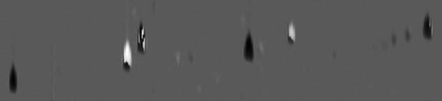
Grayscale difference image.

The grayscale difference method does an adequate job of showing the differences between the two images, but the relative context of those differences is lost because the magnitudes of the values in the comparison images are not represented in the output image (only the differences). For example, the grayscale difference does not show that the amounts of orthoxylene in the samples are relatively small, only that the difference in the amounts between the two samples is small. Another problem is the adjacent bright and dark areas in a single peak (especially for 2-hexanone). These adjacent areas with opposite colors are due to slight misregistration or slight peak shape differences.

3.2. Colorized difference

In order to make the differences between the analyzed and reference images more apparent and to retain some context for those differences, the traditional grayscale difference method is modified to color code the differences and incorporate the comparison image pixel intensities. First, the difference image is computed, just as it is for the grayscale difference method. Then, for display, the difference image is converted into a 24-bit color image (three separate bands of 8-bit integers). The color is computed in Hue-Intensity-Saturation (HIS) space [19]. The hue component of each pixel is set to pure green if the analyzed pixel value is larger or pure red if the reference pixel value is larger. The intensity component of each pixel is the maximum of the analyzed and reference pixel values, scaled to fit into the 0-1.0 range. The saturation component of each pixel is the magnitude of the difference value, scaled to fit into the 0-1.0 range. After the hue, intensity, and saturation components are calculated for each pixel, they are converted to the RGB color space and stored in a 24-bit image.

The example colorized difference image is shown in Fig. 3. The resulting color image shows brighter pixels (larger intensity) where either of the comparison images have larger values and darker pixels (smaller intensity) where both of the comparison images have smaller values, thereby retaining context for the differences that is lacking in the grayscale difference method. Pixels that have approximately equal values in both comparison images appear grayish (smaller saturation), whereas pixels for which there is a large difference have bolder colors (larger saturation). This allows the user to see simultaneously peak heights and peak differences. However, the problem of peaks with adjacent positive and negative values still is evident.

Fig. 3.

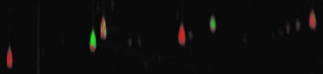
Colorized difference image.

3.3. Fuzzy difference

In practice, differences between analyzed and reference images may be caused by slight misregistration or slightly different peak shapes. It often is desirable to suppress these differences so that differences in chemical concentrations are seen more clearly. Differences due to misregistration and peak shape differences can be reduced by a new fuzzy difference comparison. Rather than comparing pixels one-by-one, the fuzzy difference method compares each pixel value in one image with the values in a small neighborhood of the other image. Note that different peak shapes may be caused by real differences in the samples or the chromatography (e.g., column degradation). Therefore, it may be worthwhile to use methods, such as the difference images, that show peak shape differences prior to using fuzzy difference visualization.

To compute the fuzzy difference between the two images, the user specifies the size of a small, rectangular window which defines a neighborhood around each pixel. The difference value at each pixel in the output image is computed using a threestep process. The first two steps compute two intermediate difference images—one comparing pixels in the analyzed image with neighborhoods in the reference image and one comparing pixels in the reference image with neighborhoods in the analyzed image. First, for each pixel, the difference is computed between that pixel value in the analyzed image and the minimum and maximum values found in the neighborhood window of the reference image. That is, for each pixel location [m, n], analyzed pixel value a[m, n], transformed and scaled reference pixel value s[m, n], and window w _s{[m, n] , the difference pixel value d _a[m, n] is:

$$\begin{array}{c}{s}_{\max }[m,n]={\max }_{[m^{\prime },n^{\prime }]\in w_{\mathrm{s}}\left\{[m,n]\right\}}\left(s[m^{\prime },n^{\prime }]\right)\hfill \\ s_{\min }[m,n]={\min }_{[m^{\prime },n^{\prime }]\in w_{\mathrm{s}}\left\{[m,n]\right\}}\left(s[m^{\prime },n^{\prime }]\right)\hfill \\ \text{if}a[m,n]<s_{\min }[m,n],\text{then}{d}_a[m,n]=a[m,n]-s_{\min }[m,n]\hfill \\ \text{else}\text{if}a[m,n]>s_{\max }[m,n],\text{then}{d}_{\mathrm{a}}[m,n]=a[m,n]-s_{\max }[m,n]\hfill \\ \text{else}{d}_{\mathrm{a}}[m,n]=0\hfill \end{array}$$

A non-zero difference is recorded only if the analyzed pixel value is either larger or smaller than all of the reference pixel values in the surrounding window. This allows the fuzzy difference algorithm to compensate for misaligned or differently shaped peaks while still showing differences in peak heights. The neighborhood window size should be set no larger than one peak width in each dimension so that pixel neighborhoods do not overlap multiple peaks. Second, the same intermediate difference algorithm is then repeated, with the analyzed and reference images swapping roles.

In the third step, the pixel values in the final fuzzy difference image are determined by whichever intermediate difference image has the largest magnitude. If the difference image that used the reference pixel as the center of each window is selected, its pixel value is negated in order to retain the same positive/negative relationship as the traditional difference image.

The fuzzy difference image can be converted to an 8-bit integer image for display, using the same method employed for the traditional grayscale difference comparison method detailed in Section 3.1. An example fuzzy difference image is shown in Fig. 4. In this image, it is clear that the internal standard, 2-hexanone, peaks have equal intensity in both images after normalization— in fact, the peak virtually disappears from the difference image. However, the grayscale shows only the difference, so, for example, the amounts of the internal standard, 2-hexanone, are not apparent.

Fig. 4.

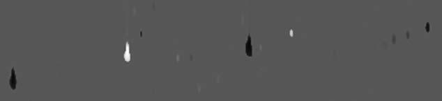
Grayscale fuzzy difference image.

The fuzzy difference image also can be displayed with the colorized difference method described in Section 3.2. The example of the colorized fuzzy difference image is shown in Fig. 5. The colorized fuzzy difference image removes many spurious differences by compensating for misaligned or differently shaped peaks and provides additional context for the difference values. For example, the peak for the internal standard, 2-hexanone, has almost no red or green, indicating the difference is small, but the whitish spot for the peak indicates its magnitude. The colorized fuzzy difference algorithm effectively highlights the most interesting differences, even where peaks are slightly misaligned or differently shaped, and it also shows magnitudes.

Fig. 5.

Colorized fuzzy difference image.

4. Tools for comparative analysis

Once comparison images have been generated for any of the image-based methods, additional tools can enhance the user’s understanding of the data.

4.1. Masking

The comparison process attempts to highlight interesting differences and suppress other differences. Users may want to mask (block) certain areas of an image so that comparisons are displayed only for a particular region(s) of the image. This is especially important if the scale of uninteresting differences is much larger than differences of interest. Masking tools allow users to delineate geometric regions or designate peak subsets to be excluded from comparison. Pixels in masked areas are set to a null value appropriate for the currently selected comparison method (e.g., gray for grayscale difference and black for colorized difference).

4.2. Tabular data

Tabular comparisons can provide quantitative information that cannot be communicated in image-based comparisons. A comparative table provides important statistical data for each pair of peaks that are uniquely identified in both the analyzed and reference image, such as volume (i.e., total response), area (i.e., number of pixels), peak retention times, and value at the peak pixel. For each feature, the values for the analyzed and reference image are listed side-by-side in the table, along with the differences (both absolute and percentage). To aid in analysis, the table rows may be sorted on any feature for either image or on any difference. The contents of the table may be saved to a file formatted as ASCII comma-separated values (CSV) for later importation into spreadsheet, database, or word-processing applications.

Table 1 shows the quantitative comparisons for the example image. For this example, the observed relative differences (from the peaks in the processed data) are nearly equal to the expected relative differences (from the relative amounts of the chemicals in the samples). In this example, the relative errors are no more than 0.20% of the total amount. As long as the peak correspondences are correct, the quantitative comparisons are as accurate as the peak quantities.

Visual comparisons and tabular comparisons each have advantages, so it is useful to navigate between the two views. If one or more peaks in the table are selected (with the mouse), those rows are graphically highlighted in the image by outlines drawn on the comparison image. This allows the user to easily locate peaks of interest, for example, the peaks with the largest volume difference or the peaks with the largest percent difference. Fig. 6 illustrates a tabular view with selected peaks and corresponding image with graphical highlights.

Fig. 6.

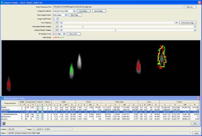
Tabular and image views with selected peak.

4.3. Three-dimensional visualization

GC × GC image data can be visualized as an elevation map, with peaks appearing as mountains. In this view, value is shown as elevation, which which allows colorization to be used for other aspects of the data. For the elevation map, the user may select one of four different images: the original analyzed image, the transformed and scaled reference image, the difference image, or an image with each pixel set to the larger of either the analyzed or the transformed and scaled reference image pixel. Masked areas or peaks are set to zero elevation. The color overlay that is draped over the surface of the elevation map can be set by the grayscale difference, colorized difference, or other difference (e.g., percentage difference, ratio, etc.). The ability to drape any comparison image over different elevation maps provides great versatility in analyzing the data. It also allows even the grayscale difference comparisons (traditional or fuzzy) to be viewed in the context of the original pixel data—something that is not possible using only a two-dimensional image. The user can then view the data from various distances or viewing angles and can locate the viewer’s position anywhere in or around the data.

A sample three-dimensional visualization is shown in Fig. 7. The data is from samples collected by Reddy et al. [3] at varying depths of the intertidal marsh sediment affected by an oil spill. (The data presented here to illustrate visualization is from preliminary runs. Subsequent runs, with improved GC × GC settings, are in [3].) The data for the analyzed image was×acquired at a depth of 0-4 cm and the data for the reference image was acquired at a depth of 16-20 cm. The subimage shown in Fig. 7 is rotated so that the n-alkanes from C₂₂form a regular pattern from right to left along the top of the image. The more polar compounds appear in the bottom of the image. The reference image was registered to the analyzed image using a peak set containing several n-alkanes, the solvent peak, and a well-separated peak among the polar compounds. The reference image was normalized to the analyzed image using a peak set of n-alkanes. This yields an image with some peaks which have nearly equal responses and some peaks which are more prominent in the reference image and some peaks which are more prominent in the analyzed image.

Fig. 7.

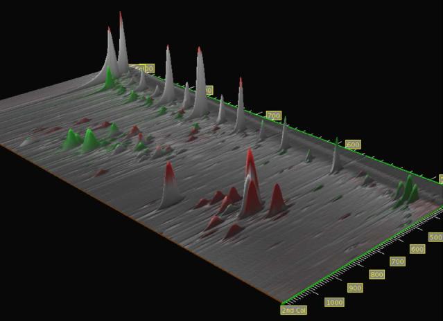
Three-dimensional rendering of a colorized fuzzy difference image draped over a maximum value elevation map.

5. Conclusion

This paper develops new methods for comparing data produced by GC × GC. Methods for registration and scaling remove incidental variations in retention times and sample amounts based on GC × GC peak metadata. A colorized difference method simultaneously shows pixel differences and pixel values. A fuzzy difference method removes incidental variations in peak shapes and peak alignments based on values in a local neighborhood. Tools for masking, tabular metadata, and threedimensional visualization significantly improve interactive analyses. Ongoing work is developing new methods for model-based GC × GC analyses and comparisons.

References

- [1].Bertsch W. J. High. Resolut. Chromatogr. 2000;23:167. [Google Scholar]
- [2].Shellie R, Marriott P, Chaintreau A. Flavour Frag. J. 2004;19:91. [Google Scholar]
- [3].Reddy CM, Eglinton TI, Hounshell A, White HK, Xu L, Gaines RB, Frysinger GS. Environ. Sci. Technol. 2002;36:4754. doi: 10.1021/es020656n. [DOI] [PubMed] [Google Scholar]
- [4].Frysinger G, Gaines R. J. Forensic Sci. 2002;47:471. [PubMed] [Google Scholar]
- [5].Welthagen W, Shellie R, Ristow M, Spranger J, Zimmermann R, Fiehn O. Metabolomics. 2005;1:57. doi: 10.1016/j.chroma.2005.05.088. [DOI] [PubMed] [Google Scholar]
- [6].Reichenbach SE, Ni M, Kottapalli V, Visvanathan A. Chemom. Intell. Lab. Syst. 2004;71:107. [Google Scholar]
- [7].Lemkin P, Lipkin L, Shapiro B, Wade M, Schultz M, Smith E, Merril C, van Keuren M, Oertel W. Comput. Biomed. Res. 1979;12:517. doi: 10.1016/0010-4809(79)90036-3. [DOI] [PubMed] [Google Scholar]
- [8].Gonzalez RC, Woods RE. Digital Image Processing. Addison-Wesley; Reading, MA: 1992. [Google Scholar]
- [9].Kunzel A. In: Lemke HU, Vannier MW, Inamura K, Farman AG, editors. Proceedings of the 13th International Congress and Exhibition on Computer Assisted Radiology and Surgery, Paris; Elsevier, Amsterdam. 23-26 June 1999.1999. p. 922. [Google Scholar]
- [10].Shi X-Q, Eklund I, Tronje G, Welander U, Stamatakis H, Engstrom P-E, Norhagen G. Engstrom, Dentomaxillofacial Radiol. 1999;28:31. doi: 10.1038/sj.dmfr.4600401. [DOI] [PubMed] [Google Scholar]
- [11].Reichenbach SE, Ni M, Zhang D, Ledford EB., Jr. J. Chromatogr. A. 2003;985:47. doi: 10.1016/s0021-9673(02)01498-x. [DOI] [PubMed] [Google Scholar]
- [12].Nadler M, Smith EP. Pattern Recognition Engineering. Wiley; New York, NY: 1993. [Google Scholar]
- [13].Ni M, Reichenbach SE, Visvanathan A, TerMaat JR, Ledford EB., Jr. J. Chromatogr. A. 2005;1086:165. doi: 10.1016/j.chroma.2005.06.033. [DOI] [PubMed] [Google Scholar]
- [14].Ni M, Reichenbach SE. In: Sandra T, Sandra P, editors. Proceedings of the 27th International Symposium on Capillary Chromatography, Riva del Garda, Italy; I.O.P.M.S, Kortrijk, Belgium. 31 May to 4 June 2004; 2004, CDROM:K.11. [Google Scholar]
- [15].Tao Q, Reichenbach SE. Peak template matching with constraint expressions for GC × GC, Gulf Coast Conference.2005. p. 66. [Google Scholar]
- [16].Rosenfeld A, Kak AC. Digital Picture Processing. second ed. Vol. 2. Academic Press; Orlando, FL: 1982. [Google Scholar]
- [17].Nelson RK, Kile BS, Plata DL, Sylva SP, Xu L, Reddy CM, Gaines RB, Frysinger GS, Reichenbach SE. Tracking the weathering of an oil spill with comprehensive two-dimensional gas chromatography. Environ. Forensics. 2006;7(1) in press. [Google Scholar]
- [18].ASTM Subcommittee D02.04.0L on Gas Chromatography . Standard Test Method for Benzene, Toluene, Ethylbenzene, p/m-Xylene, o-Xylene, C9and Heavier Aromatics, and Total Aromatics in Finished Gasoline. West Conshohocken, PA; 2002. by Gas Chromatography (D5580-02), ASTM Int’l. [Google Scholar]
- [19].Foley JD, van Dam A, Feiner SK, Hughes JF. Computer Graphics: Principles and Practice. second ed. Addison-Wesley; Reading, MA: 1990. [Google Scholar]