A theoretical investigation of the effect of predators on foraging behaviour and energy reserves

Abstract

Data show that when small birds are exposed to a model of a predator, their body mass may either increase or decrease. Although attempts have been made to explain the data using previous models, these models are based on a constant level of predation and hence are not appropriate for making predictions about the response of a bird to the sight of a predator. We have developed a novel model that includes encounters between a bird and potential predators. We show that, depending on the biology of the predator, optimal body mass may either increase or decrease. The model also makes predictions about the foraging behaviour of the bird after it has seen a predator.

1. Introduction

Several models have analysed the optimal fat levels of a small bird in winter (e.g. Lima 1986; McNamara & Houston 1990; Houston & McNamara 1993; Clark & Mangel 2000). The basis of such models is that an increase in a bird's fat reserves decreases the risk of starvation but increases the risk of predation. Starvation decreases because fat reserves provide a source of energy that can be used when foraging is not possible. Predation may increase because higher levels of fat reduce a bird's ability to escape when attacked by a predator (Hedenström 1992; Witter & Cuthill 1993). Another possibility is that metabolic rate increases with fat reserves so that more time must be spent foraging in order to maintain a higher level of reserves (McNamara & Houston 1990). During this time, the bird will be exposed to predators. A general prediction of these models is that an overall increase in predation level will decrease the optimal level of fat. Attempts have been made to test this prediction by exposing a bird to a model of a predator (e.g. Lilliendahl 1997, 1998; Pravosudov & Grubb 1998). Some experiments have found a decrease in reserves (Gentle & Gosler 2001), whereas others have found an increase (Lilliendahl 1998; Pravosudov & Grubb 1998). A problem with this procedure is that it does not correspond to the circumstances that are represented in the models. The models are concerned with how fat levels depend on a constant danger of predation. In contrast, the experiments involve a short-term increase in the danger of predation. A more appropriate way to test the models is to make use of long-term changes in predation risk. Data from the great tit, Parus major (Gosler et al. 1995), and the golden plover, Pluvialis apricaria (Piersma et al. 2003), show that winter fat levels tend to be lower in years with a high abundance of predators. Even in these cases, we note that an increase in the overall abundance of predators may not mean that predation risk is increased at all times of the day. As we show below, the effect of increased predator pressure depends on how danger fluctuates over time as a result of encounters with predators.

Birds typically stop foraging in the presence of a predator (e.g. Pravosudov & Grubb 1998; van der Veen 1999), and so the sight of a predator or a model of a predator can be viewed as imposing an interruption on them (Lilliendahl 1998; Pravosudov & Grubb 1998). Models predict that increasing the frequency of interruptions should increase optimal levels of fat (e.g. Houston & McNamara 1993), so it has been suggested that presenting a bird with a model of a predator might increase its fat reserves (Lilliendahl 1998; Pravosudov & Grubb 1998; van der Veen & Sivars 2000; Gentle & Gosler 2001; Rands & Cuthill 2001). There are two problems with viewing the presence of a predator as just an interruption. One is that a bird cannot forage during an interruption, whereas it is not forced to stop foraging in the presence of a predator. Indeed, in the model we present, there are conditions under which it is optimal to continue foraging when a predator is present. The second problem is that in models based on interruptions, the danger of predation does not depend on the time since the last interruption. In contrast, it is probable that predation risk depends on the time since a predator was last seen. We allow for such a dependency in our model.

We argue that it is not correct to use current models to make predictions about fat levels in experiments involving exposing a bird to a model predator, regardless of whether the argument is based on a change in predation pressure or interruptions. Given the discrepancy between the assumptions of current models and the procedure used in experiments, it is necessary to construct a new, richer model that explicitly includes encounters between a bird and a predator. We use such a model to investigate how the mean level of reserves depends upon predation pressure, and how the foraging intensity and level of reserves depend on the time since a predator was seen. Central to our model is the idea that the presence of predator not only acts as an interruption, but also provides information about future predation risk.

2. The model

We model the foraging behaviour of a bird over an extended period such as winter.

During this period there are two sources of mortality: starvation and predation. The bird maximizes its probability of survival over the period. (Equivalently, the bird minimizes the long-term mortality rate; e.g. McNamara 1990.)

We model the state and decision of the bird at each of the discrete decision epochs, t=0,1,2…. At each epoch, foraging may or may not be interrupted. Interruptions are caused by external influences other than predators, such as bad weather. There is no day–night cycle in the model, so interruptions caused by darkness are not included. If the bird is not interrupted at time t, it is interrupted at time t+1 with probability μ. If the bird is interrupted at time t, it is no longer interrupted at time t+1 with probability ν. Thus, interruptions last for a geometric time with a mean of ν⁻¹. Similarly, the period between interruptions, when the bird can forage, lasts for a geometric time with a mean of μ⁻¹.

Apart from whether it is interrupted, at time t the bird is characterized by two state variables:

1. its energy reserves, X(t). Reserves take non-negative integer values. If reserves fall to zero the bird dies of starvation. Under our optimal strategy, birds would not raise their reserves too high, even without an upper limit on reserves, because of mass-dependent predation. Of course, computational procedure must assume an upper limit but we have chosen a limit higher than their reserves could ever be. Therefore, the assumed limit does not act as a constraint and has no effect on the model's predictions.

2. the time since a predator was last seen, Z(t). The special case Z(t)=0 indicates that a predator is present (i.e. can be seen).

Foraging behaviour is characterized by the bird's foraging intensity, u. During an interruption, no food is available and u is constrained to be 0. When not interrupted, the bird's choice of u lies in the range 0≤u≤1.

If a bird with reserves x at time t forages with intensity u its (mean) reserves at time t+1 are:

$$x^{\prime }=x+au-b(x,u).$$ 2.1

Here au is the energy intake from food and b(x,u) is the metabolic expenditure. Computations are based on the function $b(x,u)=b_0+(b_1+b_{2}x)u$, where b₀, b₁ and b₂ are positive constants. Equation (2.1) defines the mean change in reserves. There is stochasticity about this mean, with actual reserves at time t+1 taking four possible integer values. This grid interpolation is as described in appendix 3.1 in Houston & McNamara (1999), with α taking the value 0.25.

Suppose that at time t the predator was last seen z time units ago (i.e. Z(t)=z). Then the probability that a predator is observed at time t+1 is β(z). Thus, Z(t+1) equals 0 with probability β(z), and equals z+1 with probability 1−β(z). Various forms of the function β(z) are investigated.

There is no predation risk during interruptions. Suppose that the bird is not interrupted at time t. If it last saw a predator z time units ago, the probability that a predator attempts an attack between times t and t+1 is A(z). We assume that there is, at the most, one attempted attack during this time-interval. Given that a predator attempts an attack, the probability that the bird fails to detect the predator until it is in range to mount an attack is p(u), where u is the bird's foraging intensity. If the predator does mount an attack, the probability that the attack is successful and the bird is killed is M(x), where x is the bird's energy reserves. Thus if the bird has reserves x, last saw a predator z time units ago and forages with intensity u, then it is killed by a predator between times t and t+1 with probability A(z)p(u)M(x). Various forms of A(z) are investigated. Results presented are for the case $p(u)=1-{(1-u)}^{0.3}$. This is an increasing and convex function of u that satisfies p(0)=0 and p(1)=1. Results are also based on M(x)=0.5+0.00005x².

The strategy that maximizes the probability that a bird survives the winter is found by dynamic programming (Houston & McNamara 1999; Clark & Mangel 2000). This strategy specifies how the foraging intensity of an uninterrupted bird depends on its reserves (x), the time since it last saw a predator (z), and the length of time until the end of winter. As the time to go until the end of winter increases, the optimal foraging intensity settles down to a limiting value u*(x,z) that depends on x and z, but not on the time to go or the terminal reward at the end of winter (McNamara 1990). In this paper we are concerned with this limiting behaviour.

In all our computations, for each given value of z, u*(x,z) is a decreasing function of x. When an uninterrupted animal has sufficiently low reserves, its foraging intensity is high enough to increase its reserves. When an uninterrupted animal has sufficiently high reserves, its foraging intensity is low and its reserves decrease owing to metabolic expenditure. The level of reserves at which the bird breaks even, x*(z), depends on z. For the functions that we use, β(z) and A(z) tend to non-zero limiting values as z increases. Consequently, the break-even point tends to a limiting value x** as z increases. We refer to x** as the asymptotic level of reserves. During a period in which the animal is not interrupted and does not see a predator its mean energy reserves (there are small fluctuations about the mean owing to stochasticity) tend to x**. Figure 1 illustrates the approach to x**.

Figure 1.

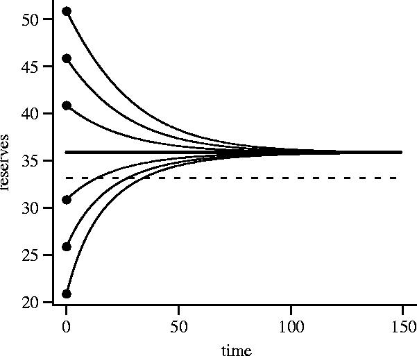
Change in mean energy reserves during a period in which the bird does not see a predator and is not interrupted. The trajectory in reserves for six different initial levels of reserves is shown. In each case, mean reserves tend to the asymptotic level x**. The overall mean energy reserves, averaged over interruption and the appearance of predators, are indicated by the dashed line. β(0)=0.8 and β(z)=0.05 for z≥1. A(z)=0.001 for all z. Other parameters: μ=0.05, ν=0.2, a=3, b₀=0.5, b₁=1, b₂=0.005.

A bird is occasionally interrupted and must stop foraging. Since energy reserves decrease during an interruption the bird will typically forage at higher intensity after the interruption ceases in order to regain lost reserves. The bird also encounters predators and may change its foraging intensity as a result. Thus, both foraging intensity and reserves fluctuate over time. We refer to the average value of reserves, averaged over interruptions and encounters with predators, as overall mean reserves. For the case illustrated in figure 1, overall mean reserves are below x**, although this is not always true (e.g. figure 2c).

Figure 2.

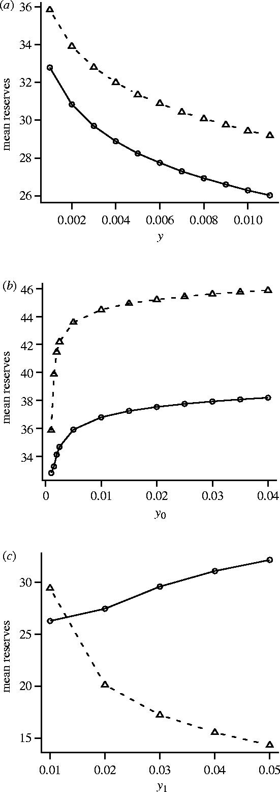
The dependence of reserve levels on predation pressure, comparing three forms of the function A(z) which specifies the probability that a predator will attempt to mount an attack. (a) Effect of y when A(z)=y for all z; (b) effect of y₀ when A(0)=y₀ and A(z)=0.001 for z≥1; and (c) effect of y₁ when A(0)=0.01 and A(z)=y₁ for z≥1. In each case two measures of reserve level are given; asymptotic reserves x** (dashed line) and overall mean reserves (solid line). In (a) and (b) β(0)=0.8 and β(z)=0.05 for z≥1. In (c) β(z)=0.2 for all z. Other parameters as for figure 1.

3. Results

(a) Effect of predation pressure on reserve levels

We consider first the case where β(z) is independent of z for z≥1. Specifically, we take β(0)=β₀ and β(z)=β₁ for z≥1. Thus, when a predator appears, the number of time-intervals for which it is present has a geometric distribution with mean (1−β₀)⁻¹. When a predator disappears, the time before it reappears is geometric with mean ${\beta }_1^{-1}$. The geometric times between the appearance of a predator might be appropriate if there were many predators, all of which were independently searching over a wide area. Then if each predator typically did not reappear for a long time, so that the next predator to appear was a different one, the probability of appearance would not depend on the time since a predator was last seen. We take A(0)=y₀ and A(z)=y₁ for z≥1 so that A(z) is also independent of z for z≥1. For this special case the time since the predator's last disappearance conveys no information about the future. In this case x*(z)=x** for all z≥1. Figure 1 is based on this case.

Most previous models that have considered the effect of predation pressure on mean energy reserves have not allowed predation risk to fluctuate in a probabilistic manner over time. Instead, there is a time-independent risk that may depend on energy reserves x and the foraging option u. We can analyse this situation within our model by assuming that y₀=y₁=y, so that A(z)=y for all z. We can then increase overall predation pressure by increasing y. Figure 2a illustrates the resulting change in the asymptotic level of reserves x** and mean reserves. As can be seen, both decrease with an increasing y. This result is in agreement with the prediction of previous models (e.g. Lima 1986; Houston & McNamara 1993).

Experimental procedures in which a bird is occasionally shown a predator are, however, best modelled by assuming a fluctuating predation risk. In figure 2b we illustrate the effect of increasing the predation risk while the predator is present, y₀. Here the predation risk when no predator is present (y₁) is held constant. As can be seen, the effect is opposite to that in figure 2a; both the asymptotic level of reserves x** and mean reserves increase with increasing y₀. In this example, increasing the predation risk while the predator is present decreases the optimal foraging intensity at a given level of reserves (figure 3a). As a consequence, the foraging intensity in the absence of a predator increases (figure 3b), since the bird must build up its reserves in anticipation of the reduced food intake when a predator reappears. The increased foraging intensity in the absence of a predator leads to higher asymptotic levels of reserves. In the example illustrated, overall mean reserves also increase.

Figure 3.

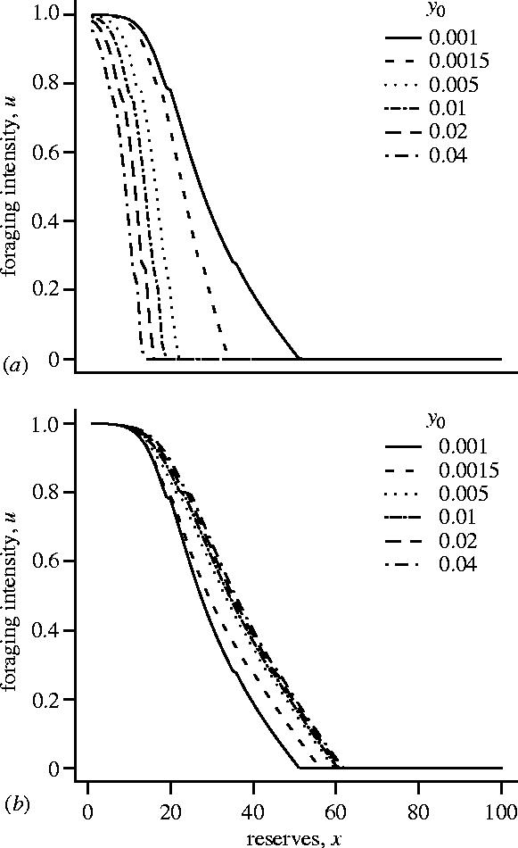
The dependence of the optimal foraging intensity u*(x,z) on reserves x, plotted for various values of y₀ for the case illustrated in figure 2(b). (a) z=0, so the predator is present and (b) z≥1 so the predator is not present.

A bird might be safer when a predator can be seen than when it cannot. This might be true when the predator is territorial, since it is only this predator that is likely to attack, and the predator cannot catch the bird unawares when it is visible (see Creswell 1996 for data on peregrines, sparrowhawks and merlins). In figure 2c we show the effect of increasing the danger while the predator is absent. In this example, the increased danger results in a decrease in the asymptotic level of reserves, but an increase in overall mean reserves.

(b) Behaviour after exposure to a predator

Several empirical studies record the foraging behaviour of a bird after a short exposure to a predator (De Laet 1985; Hegner 1985; Koivula et al. 1995; Pravosudov & Grubb 1998; Gentle & Gosler 2001). To predict the response of such a bird we suppose that before the predator appeared the bird had neither seen a predator nor been interrupted for a long time. Thus, when the predator appears, z is large and the reserves of the bird are at their asymptotic level x**. We suppose that the predator appears for a short time. This time is assumed to be too small to affect reserves significantly, so that the state variables of the bird after the predator disappears are x=x** and z=1. We then follow the future behaviour of the bird, assuming that no new predator appears and the bird is not interrupted.

In the case where β(z) and A(z) are independent of z for z≥1, we have x*(z)=x** for all z≥1. Thus the bird just maintains its level of reserves at x=x**; i.e. there is no change in behaviour after the brief appearance of the predator.

Creswell (1996) shows that if a sparrowhawk or merlin has recently attacked, it is probably still in the immediate locality. Motivated by this finding, we now assume that the variable z refers to the time since a particular predator was seen and that the probability of its return after an absence of duration z is a decreasing function of z for z≥1. Specifically, we suppose that β(0)=β₀ and

$$\beta (z)={\beta }_1+\frac{20}{100+z^2}\text{for}z\ge 1.$$ 3.1

We consider two forms of the function A(z) which specifies the probability that the focal predator will attempt an attack.

(i) Danger from the focal predator only when it is present

Assume that when the focal predator returns it becomes visible before it can attempt to mount an attack. Thus, this predator is only dangerous when z=0, when its probability of attempting to mount an attack is $\tilde{y}$. We suppose that the bird is also at risk from another type of predator that attempts to mount an attack with the same probability y₁ in all time-intervals, irrespective of when a predator of this type was last seen. We regard this additional predation risk as a given background source of mortality, and focus on the response of the bird to the appearance of the single focal predator. For simplicity, we assume that the same functions p(u) and M(x) apply to both types of predator. This scenario then corresponds to our model with $A(0)=y_1+\tilde{y}\equiv y_0$ for z=0 and A(z)=y₁ for z≥1.

Since the focal predator is noticed before it attacks, the reappearance of this predator acts as an interruption to foraging. Because β(z) decreases with increasing z, interruptions from the predator tend to occur in clusters; after one appearance another is likely to occur quickly, while if a long time has elapsed since an appearance, then the expected time until the next appearance is much longer. Consequently, immediately after the predator disappears it is optimal for the bird to forage intensively so as to raise its reserves before the predator can interrupt foraging again. However, if the predator does not reappear for a while, it is optimal to forage less intensively, and reserves gradually decline to asymptotic levels (figure 4a). Figure 4a shows reserve changes for the different mean lengths of time that a predator stays in any one appearance. As interruptions caused by the appearance of the predator last longer, the asymptotic reserve level x** increases (see caption to figure 4) and birds react more strongly to the appearance of the focal predator.

Figure 4.

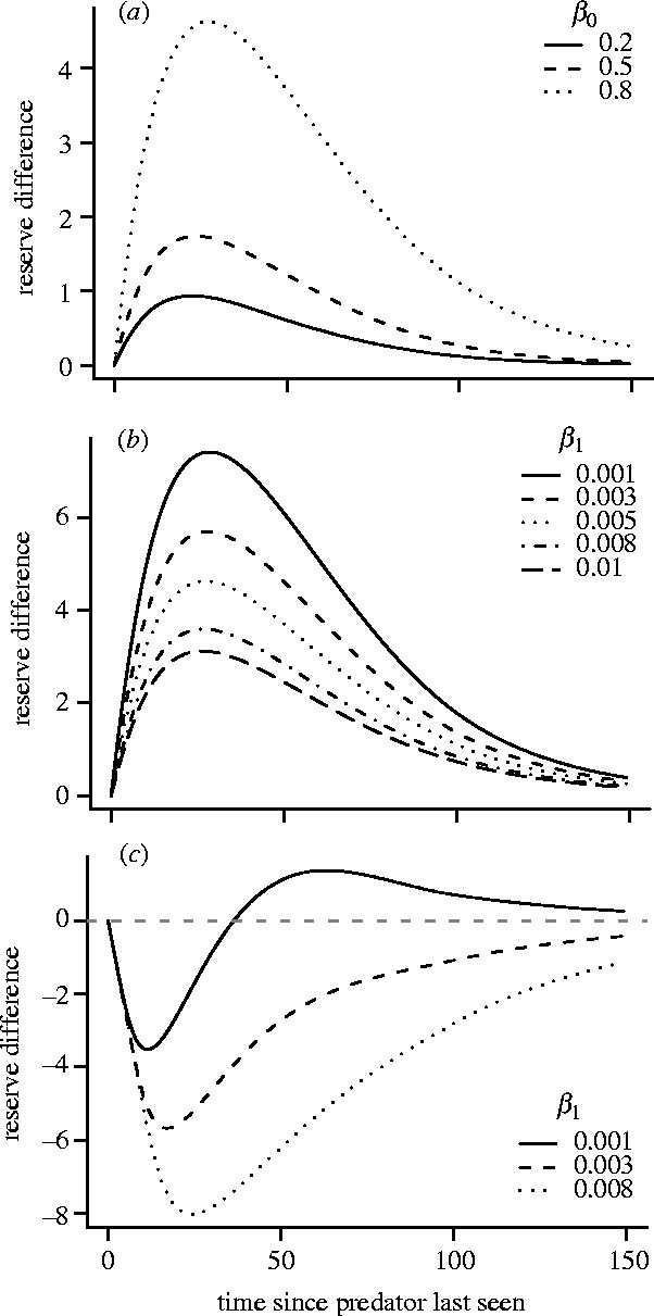
Trajectory of mean reserves after a brief exposure to a predator. In each case reserves are at their asymptotic level x** before exposure. Figures plot the subsequent deviation from x**. In all cases β(z) is given by equation (3.1). (a), (b) A(0)=0.1 and A(z)=0.001 for z≥1 and (c) A(z)=0.05β(z) for all z. In (a) x**=36.95, 38.23 and 53.64 for β₀=0.2, 0.5 and 0.8, respectively. In (b) x**=46.62, 50.70, 53.64, 56.97 and 58.75 for β₁=0.001, 0.003, 0.005, 0.008 and 0.010, respectively. In (c) x**=54.17, 65.63 and 81.28 for β₁=0.001, 0.003 and 0.008, respectively.

For the function β(z) that we are using (equation (3.1)), the probability that the predator returns in the next time unit declines towards the lower limit β₁ as the time since the predator was last seen increases. When β₁ is very small and the time since the predator was last seen is large, the existence of this particular predator is relatively unimportant to the bird and behaviour is determined by the background predation risk. Not surprisingly, as β₁ decreases, the asymptotic reserve level x** also decreases (caption to figure 4) and the change in behaviour as a result of the focal predator's reappearance increases (figure 4b). In other words, when β₁ is not small the reserves of the bird are already high in anticipation of the focal predator's return and its return has a weak effect. Conversely, when β₁ is small, the bird's reserves are not based on this predator and its reappearance demands more drastic action.

(ii) Predator attempts an attack on reappearance

Now suppose that the focal predator is the only source of predation. On its return, it attempts to mount an immediate attack with probability K, so that proportion K of reappearances coincide with an attempted attack. For this scenario we have A(z)=Kβ(z). The probability of being attacked is now highest when the predator was recently seen and decreases as the time since its last appearance increases. The bird therefore forages less intensively immediately after the predator disappears. Consequently, reserves decrease before recovering to x** (figure 4c). Figure 4c illustrates the response of the bird for three different values of β₁. As β₁ increases, so does the likelihood of return after a long absence. Since the return of the predator tends to result in a cluster of returns, with each return being followed by reduced foraging, the bird increases its asymptotic level of reserves as β₁ increases (see caption to figure 4).

4. Discussion

Whether predation risk is constant over time or depends on when a bird last saw a predator is a crucial factor in determining the effect of predation pressure. In the original models (e.g. Lima 1986; McNamara & Houston 1990; Houston & McNamara 1993), risk was constant over time and an increase in predation risk decreased reserves. In our model, this effect is illustrated in figure 2a. If predation only increases when the predator is around, the presence of a predator acts just like an interruption and reserves increase, as is shown in figure 2b. Although we do not illustrate it, in this case, mean reserves tend to increase both with the duration for which a predator is present when it appears and with the frequency of appearance of a predator (see caption to figure 4). This is what would be expected given that the presence of a predator interrupts foraging.

Since reserves fluctuate over time, there are various ways in which they can be averaged. We have chosen to present results for two forms of averaging. Overall mean reserves are an average over both interrupted and uninterrupted periods and over the presence and absence of a predator, whereas asymptotic mean reserves are an average over birds that have not been interrupted or have not seen a predator for a long time. As figure 2c shows, increased predation pressure may have different effects on these averages. In the case illustrated in this figure, it is more dangerous when the predator cannot be seen than when it can be seen. This means that the presence of a predator does not act as an interruption. These results are based on particular functions, but the qualitative patterns are robust.

There is empirical evidence that the effect of a predator on the mean mass of a bird cannot be explained in terms of the associated interruption. For example, Rands & Cuthill (2001) found that the mean reserves of blue tits during June and July increased in response to interruptions but decreased in response to simulated predation. Our model shows that encounters with predators can decrease mean reserves, but it can also produce a greater increase than expected from an interruption. This effect occurs because the presence of a predator indicates that the predator is likely to return in the near future.

The temporal response to seeing a predator depends on the information provided by this event. If the probability that a predator appears does not depend on the time since it was last seen, then the brief appearance of a predator will have little effect on the behaviour of the bird after the predator disappears. The presence of a predator may, however, make it more probable that a bird will encounter the predator in the near future. In other words, the probability of a predator appearing decreases with the time since it was last seen. In this case, the brief appearance of a predator is likely to have a significant effect on behaviour after the predator disappears, but the direction of the effect will depend on the biology of the predator. If the predator is only dangerous when seen, then there will be an increase in foraging effort after the predator disappears. Conversely, if the predator is at its most dangerous when around but out of sight, then foraging effort will decrease immediately after the predator disappears, but may later increase above its initial level (e.g. figure 4c).

If a bird is shown a predator its response depends on how it interprets this event. Our model assumes that the bird has learnt β₁. In nature, this parameter is probably never constant, and a realistic model should incorporate learning about this parameter. In a sense the model in which β(z) depends on z does this, but a realistic model would probably have the bird responding to a variable based on the last few predator appearances.

References

- Clark C.W, Mangel M. Oxford University Press; 2000. Dynamic state variable models in ecology. [Google Scholar]
- Cresswell W. Surprise as a winter hunting strategy in sparrowhawks Accipiter nisus, peregrines Falco peregrinus and merlins F. columbarius. Ibis. 1996;138:684–692. [Google Scholar]
- De Laet J.F. Dominance and anti-predator behavior of great tits Parus major: a field study. Ibis. 1985;127:372–377. [Google Scholar]
- Gentle L.K, Gosler A.G. Fat reserves and perceived predation risk in the great tit, Parus major. Proc. R. Soc. B. 2001;268:487–491. doi: 10.1098/rspb.2000.1405. http://dx.doi.org/doi:10.1098/rspb.2000.1405 [DOI] [PMC free article] [PubMed] [Google Scholar]
- Gosler A.G, Greenwood J.D, Perrins C. Predation risk and the cost of being fat. Nature. 1995;377:621–623. [Google Scholar]
- Hedenström A. Flight performance in relation to fuel load in birds. J. Theor. Biol. 1992;158:535–537. [Google Scholar]
- Hegner R.E. Dominance and anti-predator behavior in blue tits (Parus caeruleus) Anim. Behav. 1985;33:762–768. [Google Scholar]
- Houston A.I, McNamara J.M. A theoretical investigation of the fat reserves and mortality levels of small birds in winter. Ornis Scandinavica. 1993;24:205–219. [Google Scholar]
- Houston A.I, McNamara J.M. Cambridge University Press; 1999. Models of adaptive behaviour. [Google Scholar]
- Koivula K, Rytkonen S, Orell M. Hunger-dependency of hiding behaviour after a predator attack in dominant and subordinate willow tits. Ardea. 1995;83:397–404. [Google Scholar]
- Lilliendahl K. The effect of predator presence on body mass in captive greenfinches. Anim. Behav. 1997;53:75–81. [Google Scholar]
- Lilliendahl K. Yellowhammers get fatter in the presence of a predator. Anim. Behav. 1998;55:1335–1340. doi: 10.1006/anbe.1997.0706. [DOI] [PubMed] [Google Scholar]
- Lima S.L. Predation risk and unpredictable feeding conditions: determinants of body mass in birds. Ecology. 1986;67:377–385. [Google Scholar]
- McNamara J.M. The policy which maximizes long-term survival of an animal faced with the risks of starvation and predation. Adv. Appl. Probab. 1990;22:295–308. [Google Scholar]
- McNamara J.M, Houston A.I. The value of fat reserves and the tradeoff between starvation and predation. Acta Biotheor. 1990;38:37–61. doi: 10.1007/BF00047272. [DOI] [PubMed] [Google Scholar]
- Piersma T, Koolhaas A, Jukema J. Seasonal body mass changes in Eurasian golden plovers Pluvialis apricaria staging in the Netherlands: decline in late autumn mass peak correlates with increase in raptor numbers. Ibis. 2003;145:565–571. [Google Scholar]
- Pravosudov V.V, Grubb T.C. Management of fat reserves in tufted titmice Baelophus bicolor in relation to risk of predation. Anim. Behav. 1998;56:49–54. doi: 10.1006/anbe.1998.0739. [DOI] [PubMed] [Google Scholar]
- Rands S.A, Cuthill I.C. Separating the effects of predation risk and interrupted foraging upon mass changes in the blue tit Parus caeruleus. Proc. R. Soc. B. 2001;268:1783–1790. doi: 10.1098/rspb.2001.1653. http://dx.doi.org/doi:10.1098/rspb.2001.1653 [DOI] [PMC free article] [PubMed] [Google Scholar]
- van der Veen I.T. Effects of predation risk on diurnal mass dynamics and foraging routines of yellowhammers (Emberiza citrinella) Behav. Ecol. 1999;10:545–551. [Google Scholar]
- van der Veen I.T, Sivars L.E. Causes and consequences of mass loss upon predator encounter: feeding interruption, stress or fit-for-flight? Funct. Ecol. 2000;14:638–644. [Google Scholar]
- Witter M.S, Cuthill I.C. The ecological costs of avian fat storage. Phil. Trans. R. Soc. B. 1993;340:73–92. doi: 10.1098/rstb.1993.0050. [DOI] [PubMed] [Google Scholar]