Using the quantitative genetic threshold model for inferences between and within species

Abstract

Sewall Wright's threshold model has been used in modelling discrete traits that may have a continuous trait underlying them, but it has proven difficult to make efficient statistical inferences with it. The availability of Markov chain Monte Carlo (MCMC) methods makes possible likelihood and Bayesian inference using this model. This paper discusses prospects for the use of the threshold model in morphological systematics to model the evolution of discrete all-or-none traits. There the threshold model has the advantage over 0/1 Markov process models in that it not only accommodates polymorphism within species, but can also allow for correlated evolution of traits with far fewer parameters that need to be inferred. The MCMC importance sampling methods needed to evaluate likelihood ratios for the threshold model are introduced and described in some detail.

1. Introduction

In 1934, Sewall Wright introduced the threshold model (Wright 1934a), which he applied (Wright 1934a,b) to modelling the genetics of the number of toes on the hind foot of guinea pigs. It posited a discrete character with a limited number of states (Wright used at least three, but in this paper I will confine attention to two states). There is polygenic genetic variation on an invisible underlying scale, which has come to be called the liability. The states of the observable scale, which I call 1 and 0, depend on whether the underlying liability is or is not above a threshold value. Since the underlying scale is arbitrary, it is convenient to place the threshold at zero, and it is also convenient to assume that the variance of the population's liability values is unity. Wright used the model to fit the frequencies of extra hind digits in crosses between inbred strains of guinea pigs, trying to explain results of a large number of crosses by inferring the mean liabilities of the individual strains.

An alternative way to express the model (used by Curnow & Smith 1972) is that the genetic effects produce a liability x, with the probability of the observed phenotype 1 being the integrated normal distribution Φ(x) evaluated at this value. This is equivalent for a single trait and a single individual, but not for two traits or two individuals, where the most straightforward interpretation of this alternative would seem to rule out environmental correlations. I will avoid this alternative framework in this paper, preferring to have the environmental effect added on the liability scale.

The threshold model has seen a certain amount of use in human genetics, much of it as a result of the work of Falconer (1965, 1967). There it is fitted to data on the incidence of a trait among relatives of affected individuals. A useful review of this is given by Lynch & Walsh (1998, ch. 25). A more extensive review is given by Curnow & Smith (1972). Figure 1 shows the threshold model, with the underlying liability trait as well as the observed discrete phenotype.

Figure 1.

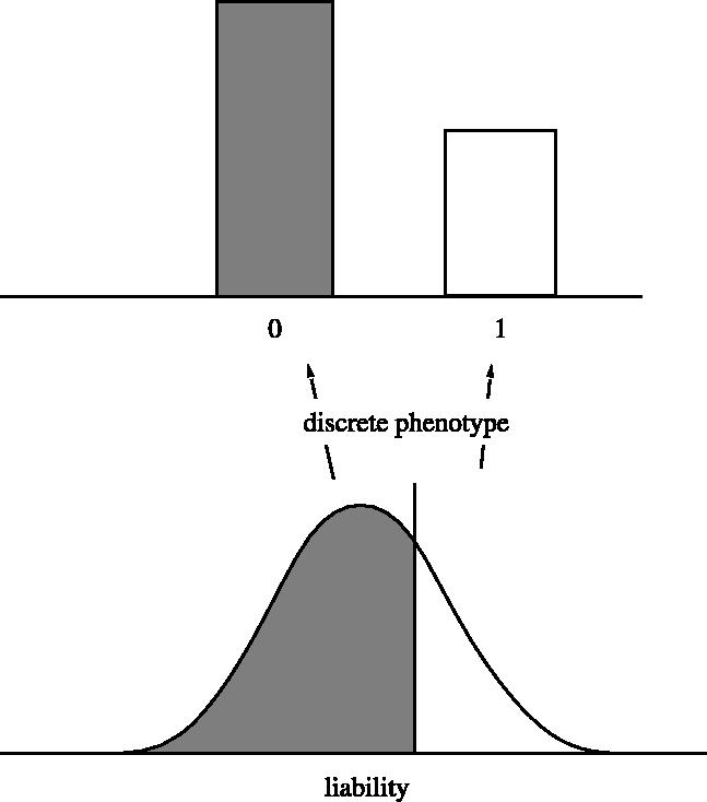
The threshold model of quantitative genetics, showing the continuous distribution of the underlying liability characters, and the resulting discrete distribution of the observed phenotype.

In this paper I will discuss prospects for adapting the threshold model to between-species inference, without losing the connection to quantitative genetics. Nonetheless, that connection becomes rather tenuous. In particular, I explore prospects for using statistically efficient methods (maximum likelihood and Bayesian inference).

2. Likelihood and Bayesian inference

As computationally intensive methods became possible, likelihood and Bayesian methods have gained ground in many areas of statistics. In the quantitative genetics and human genetics literature, they have become the standard against which all other methods are measured. The threshold model has had to await this recent wave of interest in computationally intensive methods, as its mathematics resists simpler computations. Consider a pedigree of n individuals, some of them scored for p 0/1 characters. Suppose that these are determined by underlying liabilities, according to a threshold model. We must allow the liabilities to have the usual genetic and environmental variance components, and to be correlated in an arbitrary fashion.

If the additive genetic, dominance, and environmental variance components lead to an overall covariance matrix C, we can imagine computing the likelihood for the pedigree, assuming that the threshold on each liability scale is at 0. The joint density function of the vector of liabilities x is of course the multivariate normal density

$$\varphi (\mathit{x};\mathit{\mu },\mathit{C}),$$ (2.1)

where μ is the vector of means of the liabilities. This is an np-dimensional density.

If the observed discrete {0,1} phenotypes for the n individuals are called the y_ij, this being the phenotype of the jth character of the ith individual, the likelihood is the joint probability of these. This is the multiple integral of the density function over the region of the space of liabilities lying on the proper sides of all the thresholds

$$L=\text{Prob}(\mathit{y};\mathit{\mu },\mathit{C})=\underset{x_{11}\in R_{11}}{\int }\underset{x_{12}\in R_{12}}{\int }\dots \underset{x_{1p}\in R_{1p}}{\int }\underset{x_{21}\in R_{21}}{\int }\dots \underset{x_{np}\in R_{np}}{\int }\varphi (\mathit{x};\mathit{\mu },\mathit{C}),$$ (2.2)

where the regions of integration R_ij are each either (0, ∞) if y_ij=1 or (−∞, 0); if y_ij=0. In other words, the likelihood is a high-dimensional integral of a corner of a correlated multivariate normal distribution. It is a function of parameters that include the means and the additive, dominance and environmental variances and covariances between characters. Our objective will be to calculate likelihoods or likelihood ratios for different parameter values or, in the Bayesian case, to infer the posterior distribution of these parameters.

There are approximations for such integrals, but they work well only when the number of variables is modest. Harville & Mee (1984) described maximum likelihood inference in mixed models using the threshold model, but they were forced to retreat to approximate evaluation of the necessary integrals. As with many high-dimensional integral problems, this one has had to await Monte Carlo sampling methods such as Markov chain Monte Carlo (MCMC) for effective treatment.

3. Monte Carlo sampling methods

McCulloch (1994) described the use of MCMC sampling methods for the threshold model with a mixed model underlying it. This model includes as special cases most of the ones we will be interested in. McCulloch's general strategy is to sample liabilities, using an MCMC method known as a Gibbs sampler and, by doing this many times, to approximate the likelihood. A similar strategy allows the approximation of the posterior if one is doing Bayesian inference. McCulloch's particular method uses an EM (expectation–maximization) algorithm to update parameter values. A Bayesian approach to a similar problem was made by Sorenson et al. (1995), also using an MCMC method with Gibbs sampling.

These applications of the MCMC sampling make the threshold model useable for pedigree data in quantitative genetics. Using these approaches, it is possible to infer genetic variances and covariances from pedigree data with multiple discrete traits. These methods are part of the increasing use of MCMC methods for likelihood and Bayesian inference in quantitative genetics, enabling estimates and inferences for models that would be intractable otherwise. In this paper, I will discuss application of the threshold model to between-species data. First, it may be helpful to explain the MCMC methods more generally.

4. Monte Carlo integration

We are approximating a high-dimensional integral for which no closed-form formula exists. In the case of pedigree data, we would be integrating over the unknown values of the liabilities of individuals in the pedigree, both individuals that we have observed and those that we have not observed. The integral is approximated by Monte Carlo integration—drawing a large sample of points from the domain of integration and evaluating the contribution to the integral in the vicinity of these points by evaluating the function at the points. In effect, we replace the continuous function that is being integrated by a histogram that approximates it.

Monte Carlo integration can be very effective, but if most of the area under the function is in a very restricted part of the domain, a naive Monte Carlo approach can fail because most of the samples are taken from nearly irrelevant areas. The solution to this problem is to sample non-randomly, concentrating the sample mostly in the region that contributes most to the integral. This is importance sampling. One needs to correct for the concentration of the sampling by down-weighting each sample so that it counts correspondingly less. Importance sampling has been a staple of Monte Carlo integration since its (re)discovery in the 1950s.

5. Markov chain Monte Carlo

MCMC integration has been around almost as long, but has been used most widely since the 1980s, when increasing computer power made it practical. It uses a specially constructed Markov process to wander through the domain of integration, sampling points in a way that is guaranteed to achieve the desired importance sampling distribution, if one runs the chain long enough. The issue of how long to run the chain is particularly important, as the samples from the domain of integration are not independent, and if the sampler gets stuck in one region while never sampling another highly relevant region, the result can be misleading. While various diagnostic statistics have been proposed to assess whether the chain has reached stationarity, these work well only when there are no isolated peaks. Without analytical insight, we cannot guarantee that over the horizon there is not a major peak awaiting discovery.

6. Importance sampling

To use MCMC methods, we would sample from an importance sampling density over liabilities, and then correct for the fact that the importance sampling has overconcentrated on some regions. The usual importance sampling correction when the true density of liabilities is f(x) and the importance density we choose is g(x), and when we integrate a function h(x), is simply to note that the integral is the expectation of the function h(x) over the density f(x). This can be written as the expectation of (f(x)/g(x))h(x) if the points are drawn from the density function g(x) instead of f(x)

$${\mathbb{E}}_f[h(\mathit{x})]=\underset{\mathit{x}}{\int }f(\mathit{x})h(\mathit{x})=\underset{\mathit{x}}{\int }g(\mathit{x})\frac{f(\mathit{x})}{g(\mathit{x})}h(\mathit{x})={\mathbb{E}}_g\left[\frac{f(\mathit{x})}{g(\mathit{x})}h(\mathit{x})\right].$$ (6.1)

We choose values of x from g(x), and then average ( f/g)h for them.

We will be interested in computing the likelihood at an arbitrary value θ of the parameters, when sampling given a different value, our ‘driving value’ θ₀. The likelihood is the integral over the region of x corresponding to the observed {0,1} phenotypes. We can thus write it as the integral over the whole region of an indicator variable I_y(x) which is 1 whenever the liabilities x are such that the correct phenotypes y are obtained.

7. Importance sampling methods

(a) The naive method

There are many possible importance sampling schemes. One of the least useful is to draw from the prior density of liabilities unconditioned on the data, which is f(x; θ₀). The above formula then tells us that we can estimate the likelihood for any other value of θ by averaging $f(\mathit{x};\mathit{\theta })/f(\mathit{x};{\mathit{\theta }}_0)I_{\mathit{y}}(\mathit{x})$ over all the values of the liability that we sample. Most of the time, these liabilities are outside the relevant region, so that I_y(x) is 0, and we can waste vast amounts of time sampling.

(b) Sampling conditional on the data

A much more useful importance sampling density is to draw the x from the conditional distribution of x given y. That density is

$$g(\mathit{x};{\mathit{\theta }}_0)=\text{Prob}(\mathit{x}|\mathit{y},{\mathit{\theta }}_0)=\frac{I_{\mathit{y}}(\mathit{x})f(\mathit{x};{\mathit{\theta }}_0)}{\underset{\mathit{x}}{\int }{I}_{\mathit{y}}(\mathit{x})f(\mathit{x};{\mathit{\theta }}_0)}.$$ (7.1)

The likelihood for some value of θ, usually somewhat different from our current value θ₀, is

$$L(\mathit{\theta })=\underset{\mathit{x}}{\int }f(\mathit{x};\mathit{\theta })I_{\mathit{y}}(\mathit{x}).$$ (7.2)

The denominator in equation (7.1) when we use it to compute this quantity turns out to be simply L(θ₀). Using that, we can imagine doing the importance sampling and getting the likelihood as an expectation over that sampling. Since g(x; θ₀) is the conditional distribution of x given the y, it has zero density of x everywhere except where the observed values of y are consistent with the x. We can then omit the I term in the expectation, as it is 1 for all the sampled values of x.

$$L(\mathit{\theta })={\mathbb{E}}_{g(\mathit{x};{\mathit{\theta }}_0)}\left[\frac{f(\mathit{x};\mathit{\theta })}{f(\mathit{x};{\mathit{\theta }}_0)/L({\mathit{\theta }}_0)}\right].$$ (7.3)

Moving the L(θ₀), this can be written as

$$\frac{L(\mathit{\theta })}{L({\mathit{\theta }}_0)}={\mathbb{E}}_{g(\mathit{x};{\mathit{\theta }}_0)}\left[\frac{f(\mathit{x};\mathit{\theta })}{f(\mathit{x};{\mathit{\theta }}_0)}\right].$$ (7.4)

The likelihood is then approximated by sampling n times from g(x; θ₀) and averaging the ratio of f's

$$\frac{L(\mathit{\theta })}{L({\mathit{\theta }}_0)}\approx \frac{1}{n}\sum _{i=1}^n\frac{f({\mathit{x}}_i;\mathit{\theta })}{f({\mathit{x}}_i;{\mathit{\theta }}_0)}.$$ (7.5)

As this approximates the likelihood ratio, we can afterwards find an improved estimate of θ by maximizing it. For this to make a good estimate of the shape of the curve of likelihood ratios, and hence of the value of θ that achieves the maximum likelihood, the driving value θ₀ should be close to the maximum likelihood value. This strategy has been used in coalescent-based likelihood models for population samples of molecular sequences (Kuhner et al. 1995), and we have applied it in subsequent papers to models with a variety of evolutionary forces. One has to run MCMC chains multiple times, each time maximizing θ to get the driving value for the next chain. Although there is no mathematical guarantee of convergence as there would be if this were an EM algorithm, this method can do well.

Note that equation (7.4) computes the likelihood ratios for a variety of values of θ using the same set of samples of the x_i. Thus the estimated curve of likelihood ratios is smooth, avoiding the jaggedness that would result from using a separate simulation for each value of θ.

Our ability to do all this depends on being able to sample from the conditional distribution of x given y. There are several approaches to this. It may be useful to mention some of them.

(c) The Gibbs sampler

If the x are vectors with many components, one can update one component at a time. If we choose x_i from the conditional distribution of that component given the values of all the others, then if appropriate conditions hold we have a Markov chain that will achieve the joint distribution of x. This is called a Gibbs sampler; it was introduced by Geman & Geman (1984). In the present case we will be using it to update underlying liability values, conditional on the phenotype values y.

(d) The Metropolis–Hastings sampler

If we could not draw samples from the conditional distribution of some of the x_i given the others and given the phenotypes, we could instead use a rejection method, the Metropolis–Hastings method (Metropolis et al. 1953; Hastings 1970). The Metropolis sampler draws nearby points from a proposal distribution, rejecting them if a uniform random fraction between 0 and 1 turns out to be greater than g(x_new)/g(x). If the proposal distribution is biased, the Hastings correction alters this rejection formula to counteract the bias. Metropolis–Hastings sampling was used by Kuhner et al. (1995). In the present case it will not be necessary, as an approximation to a Gibbs sampler succeeds, though with some reweighting needed to implement it.

There are a number of other major families of sampling methods. Which one of these samplers is required depends on the details of our model, to which we now turn.

8. A between-species application

As we have seen, quantitative geneticists have a head-start in inferring parameters of the threshold model from pedigree data within species. There are in addition interesting possibilities in between-species data; these may help to bring morphological systematics and quantitative genetics into fruitful contact. Instead of pedigrees of individuals, we will be dealing with phylogenies (evolutionary trees) of species.

(a) Discrete characters in systematics

It is common for systematists and morphologists to encounter characters that have discrete states, with different species having different states. (It is less common for them to record polymorphisms of these states, though it does happen.) Traditionally, when inferences are made of phylogenies, this is done by parsimony methods, which try to explain the evolution of these states by finding that phylogeny that can allow them to evolve with the fewest changes of state. Parsimony methods have the defect that they can be statistically inconsistent when there are rate inequalities among lineages. If the number of states is large, so that accidental convergence on the same state is unlikely in different lineages, they can behave acceptably. If rates of change are low they generally behave well, and are robust to variation of rates of change from character to character. In general, a more statistical method is needed. My book (Felsenstein 2004) can be consulted for references.

Recently, some attempts have been made to model the evolution of these characters, using the sorts of stochastic models used in modelling the changes of state in DNA sequences. Pagel (1994) used a discrete {0,1} stochastic model for each character, and proposed to use likelihood ratio tests to discover whether two characters change independently. Lewis (2001) applied a similar k-state model, assuming that evolution is independent in different characters. In their models, the population mean is represented by a single value, which has a Markov process undergoing sudden changes on the scale of observed phenotypes. In the threshold model, the underlying liability scale shows gradual changes.

There is no polymorphism possible in the Pagel's and Lewis's discrete stochastic model, as there is in the threshold model when the population mean is in the vicinity of the threshold. If the data were not simply a single state for each species, but rather gave the discrete phenotypes of a sample of individuals from each species, the threshold model could be used to carry out likelihood inference in a straightforward way, as we shall see below.

Another difficulty with discrete models in which a population makes a transition from one state to another instantaneously is that it is difficult to allow for covariation among characters. Pagel's method allows for it, but in a way that would become cumbersome if there were more than two characters covarying. Thus, with even as few as 10 characters, one might need 1023 different parameters to allow state combinations at other characters to affect the rate of evolution or the equilibrium frequencies of the states at a character. Lewis's model does not attempt to correct for non-independence of characters.

By contrast, we will see that the threshold model can allow for covariation of characters, with far fewer parameters. If the underlying liabilities covary in their evolution, they will have only p(p+1)/2 covariances. In the case of 10 characters this would be 55 parameters. For cases in which individual phenotypes are collected from a sample within each species, another set of covariances can be inferred, the phenotypic covariances of characters among individuals.

(b) A between-species threshold model

Imagine a species with a {0,1} character determined by a threshold model. As time goes on, gene frequencies will change by genetic drift and by natural selection. To know how they change would take a detailed model, which is usually lacking. As the gene frequencies of the many loci underlying the liabilities change, the distribution of liabilities on their axis wanders back and forth. In some populations the mean will be far to one side of the threshold, and those populations will have their discrete phenotype values all 1 or all 0. In some populations it may be near the threshold, and those populations will show polymorphism, with both 1 and 0 phenotypes found.

In the absence of a detailed model of the changes of gene frequency, we can model the changes by having the mean of the liability wander on its scale according to a Brownian motion. This model was used by Edwards & Cavalli-Sforza (1964) for change of gene frequencies in phylogenies of populations, and extended by me (Felsenstein 1973, 1981) to change of quantitative characters in phylogenies of populations or species. In the latter case the changes may be caused by genetic drift or by temporally variable selection. I will use Brownian motion to model change of the underlying p liabilities of p observable discrete {0,1} characters in a set of related species. They will be assumed to have the mean liabilities change by Brownian motion along the branches of phylogeny. The variance of the distribution of liabilities within each population will be assumed to remain constant, so that all species have the same within-species variance. A simulation of this model on a simple tree is shown in figure 2.

Figure 2.

A simulation of a threshold model with one character, evolving by Brownian motion of the liability on a simple five-species tree. Each lineage is shaded to indicate the proportion of individuals in state 1 (shown by black shading). The upper two species end up with polymorphism, the middle species nearly all with state 0, and the lower ones nearly all with state 1.

Two properties of this threshold model seem intuitively reasonable.

1. It allows for polymorphism. Whereas the stochastic two-state model represents each lineage as having only a single state, the threshold model envisages a population with variation in the liability, which implies for each lineage population frequencies of the two states. When the mean liability is far from the threshold, only one state is likely to be found in any sample. But as the population crosses the threshold, it should be notably polymorphic.

2. The rate of change between states varies through time. In the stochastic two-state model, the probability of transition to the other state is the same, no matter how long the lineage has been in its current state. But under the threshold model, the probability that a lineage will be predominantly one state depends on mean liability. Immediately after the mean of the lineage has crossed the threshold, it is quite likely to recross it again. Later on, the mean may have wandered far into the region on that side of the threshold, which makes it much less likely to recross the threshold soon. Opinions may differ on whether this will hold for actual discrete characters; to me this property ‘feels’ right.

A limitation of the Brownian motion threshold model is that the amount of genetic variation on the liability scale is held constant. One would want to allow it to change: as genetic drift eliminates variation of the liability and mutation restores it, the variance of the liability character should make excursions down and up. Although it will have a long-term equilibrium value, there will be periods when variability is greater than at other times. I have abstracted away from this degree of realism in the interest of tractability. A varying amount of variability would lead to a random walk whose rate of motion varied through time, the rate being autocorrelated. Varying selection pressures are another possible source of autocorrelation. I do not know a sensible way of modelling these phenomena in a way that is tractable. Adding another hidden variable for the amount of variation seems likely to get the MCMC bogged down, with too much sampling needed. So for the present I will have the motion of the mean liability be Brownian, which implies that the amount of variation in the population remains rigidly constant.

The Brownian motion is of p correlated variables, with no assumption that they have equal variances or that they are independent. I have explained in some detail in a number of places (Felsenstein 1988, 2002, 2004) where the covariances of evolutionary change come from. They are the result of both genetic covariances and selective covariances. The former are the standard additive genetic covariances of quantitative genetics; the latter are covariances of the selection pressures through time. While the additive genetic covariances could in principle be inferred by standard quantitative genetics breeding experiments, the selective covariances would only be available by inferring the overall covariances of evolutionary change by fitting the species data to a tree, and then removing the effect of the additive genetic covariances and seeing what was left. Direct inference of the selective covariances would only be possible if a detailed mechanistic model of the functional ecology of the character were available.

We will look into the possibilities of treating two problems.

1. Given a phylogeny provided by molecular data, to infer the covariance matrix of evolutionary changes. This is analogous to quantitative genetic investigation of realized selection pressures and realized heritabilities.

2. Given only the discrete characters, to infer the phylogeny as well as the covariance matrix of evolutionary changes. One must be continually alert to the danger of overfitting here, as the number of quantities inferred is substantial.

In both cases we will need to have some way of sampling the liabilities. There are two distinct cases for this sampling: interior nodes of the tree for which no phenotype has been observed, and tips of the tree for which a phenotype is known.

(c) Updating interior nodes

For each node on the tree, if we reconsider its liability, we will find that it is conditional on the liabilities of its immediate neighbours. If an interior node of a tree is reconsidered, it will typically have three such neighbours: two descendants and its ancestor. Recalling that the liabilities for the different characters are correlated in our model, it will be a great advantage if we can transform them to independence. This is easily done: if the covariance matrix of evolutionary change is C, we can use Cholesky decomposition (cf. Press et al. 1992, section 2.9) or spectral decomposition to find a matrix A which is its square root, so that C=AA^T. Using its inverse, a new vector of characters z=A⁻¹x can be computed that will all evolve at equal rates and independently. As a transformation of the liabilities, they will be unobserved, but being transformed they do not individually determine the observed discrete phenotypes.

On this transformed liability scale, updating interior nodes can easily be carried out by Gibbs sampling. Each coordinate is conditional only on that coordinate in its immediate neighbours. I will show elsewhere that, if the branches leading to the three neighbours have lengths v₁, v₂ and v₃, and if for a coordinate of the transformed liability their values are z₁, z₂ and z₃, the conditional distribution of z at the node is simply normal, with mean

$${\mu }_z=\frac{\frac{1}{v_1}{z}_1+\frac{1}{v_2}{z}_2+\frac{1}{v_3}{z}_3}{\frac{1}{v_1}+\frac{1}{v_2}+\frac{1}{v_3}}.$$ (8.1)

The neighbours' values are weighted inversely by the variance that would be expected to accumulate along the branches leading to them. The variance of the transformed liability z is given by

$${\sigma }_z^2=\frac{1}{\frac{1}{v_1}+\frac{1}{v_2}+\frac{1}{v_3}}.$$ (8.2)

Having the mean and variance of z, we can draw from its distribution. This is a Gibbs sampler. The new value is always accepted. It can be used to update the interior nodes of the tree, updating all the transformed liabilities z.

(d) Updating tips

At the tips, the liabilities cannot be updated as easily. We need to ensure that the liabilities reconstructed at the tips are consistent with the observed discrete phenotypes. To do this we need to be back on the original liability scale. We want to construct a Gibbs sampler for the liabilities at the tips. Some methods suggest themselves.

The first draws liabilities at the tip conditioned on the liabilities at the nearest internal nodes, but not conditioned on the observed characters. The liabilities drawn are then rejected if they are not consistent with the observed characters, and the process is repeated. Finally, a set of liabilities for the tip is drawn that are consistent with the observed phenotypes. If we could do this, it would be an exact Gibbs sampler.

Suppose that we have a tip with an observed phenotype y_i in character i. Its nearest neighbour is an interior node. We can take the transformed liabilities z at that interior node and use them to draw transformed liabilities for the tip. If the branch length between these two nodes is v, the ith coordinate of the transformed liability at the tip is obtained by adding a normal variate with mean 0 and variance v to the corresponding transformed liability at the interior node.

However, this does not condition on the observed discrete phenotype at the tip. To do that, we could transform the newly drawn liabilities at the tip back to the original liability scale, using the transformation A, and see whether they then lie on the correct sides of the thresholds in each character. One convenient way is to have A defined by the Cholesky decomposition, because it is then a triangular matrix. As we compute each successive liability coordinate x_i for the tip, we continue only if it lies on the proper side of the threshold. This is straightforward, but leads to a large fraction of cases in which we have to reject the sampled transformed liabilities, because they produce liabilities that lead to the wrong discrete phenotypes. We then have to continue, sampling new sets of zs, until we get one that leads to the observed phenotypes. This can be quite tedious and become bogged down with even a moderate number of characters. Once it succeeds in sampling a set of xs from the relevant region, it does carry out a Gibbs sampler step.

It would be desirable to do the sampling in some way that conditioned on getting xs that were in the appropriate region. We can factor conditional probability of the x_i given the y_i into terms for the probabilities of the individual x_i, each given the previous x_i

$$\begin{array}{lll}\text{Prob}(\mathit{x}|\mathit{y})\hfill & =\hfill & \text{Prob}(x_1|\mathit{y})\text{Prob}(x_2|x_1,\mathit{y})\hfill \\ \hfill & \hfill & \text{Prob}(x_3|x_1,x_2,\mathit{y})\dots \hfill \\ \hfill & \hfill & \text{Prob}(x_p|x_1,x_2,\dots ,x_{p-1},\mathit{y}).\hfill \end{array}\}$$ (8.3)

The conditioning on the full set of y_i at each stage still prevents convenient sampling using this formula. We might be tempted to simplify further and compute

$$\begin{array}{lll}P(\mathit{x})\hfill & =\hfill & \text{Prob}(x_1|y_1)\text{Prob}(x_2|x_1,y_2)\hfill \\ \hfill & \hfill & \text{Prob}(x_3|x_1,x_2,y_3)\dots \hfill \\ \hfill & \hfill & \text{Prob}(x_p|x_1,x_2,\dots ,x_{p-1},y_p).\hfill \end{array}\}$$ (8.4)

If this were the equivalent to equation (8.3), it would allow us to sample the x_i easily. It is not too hard to sample from the appropriate tail of a univariate normal density. Using the triangular form of matrix A, we would draw x₁ from the appropriate tail of a normal distribution that had the correct mean and variance. Then, knowing x₁, we would calculate the mean and variance for x₂, draw it from the appropriate tail of its normal distribution, and continue in this way until we had drawn all of the x_i.

Unfortunately, we cannot simply do this, because the conditioning in equation (8.4) is not equivalent to that in equation (8.3). The quantities Prob(x|y) and P(x) are not equal. The matter has not been tested yet, but we may be able to use the series of draws from the tails of univariate normal distributions, if we compensate for the inaccuracy by reweighting the results. Having drawn a point x (the liabilities of the p characters), we can evaluate the quantities Prob(x|y) and P(x) and then assign the outcome x of the draws of liabilities a weight equal to the ratio

$$w(\mathit{x})=\text{Prob}(\mathit{x}|\mathit{y})/P(\mathit{x}).$$ (8.5)

To be more precise, we cannot actually compute the conditional density Prob(x|y), because we do not know the normalizing constant that would make its integral 1. But that will simply mean that the weights will be off by a common factor. For the uses we will make of them, this will not cause any difficulty. The likelihood computations then involve a weighted sum of ratios, extending the formula in equation (7.5). The danger is that many of the sampled sets of liabilities would lead to a low weight, with only a small fraction of them dominating the resulting calculation. That would lead us to need to take a very large number of samples to get accuracy. This is a special concern since the overall weight of a complete set of liabilities would be the product of the weights at the individual tips.

The sampling using these weights is not precisely a Gibbs sampler, but rather an importance sampling approximation to one. There is more to be done in trying different sampling strategies for liabilities. For the moment the issue awaits appropriate trials.

9. Inferring the covariances

One of the chief reasons for computing likelihood ratios in this model is to infer the covariance matrix of the liabilities, which gives the covariances of evolutionary change. There may be many reasons for wanting to infer and test covariances; one is simply to test whether two characters show correlated evolutionary changes across a set of species.

Given efficient strategies for sampling liabilities, these can be used to make approximate maximum likelihood estimates of the covariances of evolutionary change. With each new set of liabilities, we have an observed set of reconstructed changes along each branch of the tree. If we know the length v of a branch, and if liabilities i and j show values x_i and x_j at one end of the branch and ${x^{\prime }}_i$ and ${x^{\prime }}_j$ at the other, then the contribution of this branch in this sample of liabilities to the estimate of the covariances is simply $(x_i-{x^{\prime }}_i)(x_j-{x^{\prime }}_j)/v$ for the covariance between liabilities i and j. The estimate of the covariance is an average of this over all branches. Taking a large number of sets of liabilities, we average these, and then we can update our inference of the covariance matrix C of evolutionary change.

That strategy is related to an EM algorithm. If we could observe the x_i directly, our maximum likelihood estimate of the covariance matrix C would be these observed covariances of character changes over branches, as above. The EM algorithm uses the expectation of the sufficient statistics (in this case the observed scaled covariances of changes) given the observed phenotypes at the tips. These expectations are taken using the current estimates of the parameters. Those current estimates are then replaced by the new estimates, and the process continues until it converges, ultimately making a maximum likelihood estimate.

In the present case, we have driving values of the parameters, and we take a large (but not infinitely large) sample of the liabilities. The averages of the observed covariances can be made. If the resulting covariances then replace the driving values, and the process is repeated, one is approximately undertaking an EM algorithm, which should ultimately arrive in the vicinity of a maximum likelihood estimate. It will never totally settle down, because the finiteness of the sample of sets of liabilities makes for some wandering about.

It will also be possible to approximate the likelihood surface for the elements of the covariance matrix. This should allow approximate likelihood ratio tests of assertions about the covariances.

10. Searching among trees

Inferring the covariances C is simple compared with the case where one also wants to infer the tree. It would be possible to update both liabilities and tree topologies. If one erased the tree structure in an interior region of the tree, proposed a new topology there, and also filled in liabilities in that region, one could do Metropolis–Hastings rejection sampling. If we use a prior distribution of trees, it is straightforward to compute the joint probability of the tree and the liabilities both before and after the change. The ratio of these probabilities would be used for Metropolis–Hastings sampling, to sample from a posterior distribution of trees. If one did not want to do Bayesian inference, one could correct for the assumed prior on trees and use the Bayesian sampling strategy to characterize the likelihoods of trees.

The chief complication is that one would want to change the estimates of the covariances as one changed the tree. This is a much messier matter than altering the tree; it is a major barrier to developing such a method. The matter needs careful testing, and there are many developments ahead. As we are inferring both the covariance matrix and the tree topology, there may be rather little statistical power available. I have presented elsewhere (Felsenstein 2002) degrees of freedom calculations showing for which combinations of numbers of species and numbers of characters there is any power available to infer both covariances and topologies. The larger the number of characters, the more difficult it is to infer both, as the number of parameters needed rises as the square of the number of characters.

It seems likely that the greatest use of the threshold model will come when we have a reasonably good estimate of the phylogeny from molecular data, and need not rely on the morphology for that inference. We can then use the MCMC machinery to infer covariances of the evolution of the liabilities across that known phylogeny. It would also be possible (cf. Felsenstein 1988) to use a sample of bootstrap estimates of the phylogeny, and infer covariances for each. This should correct for the uncertainty of the inference of the phylogeny.

11. Polymorphic characters

If, instead of a single state (0 or 1) for each character in each species, we had observations on individuals, we could use the threshold model to fit these data. Allowing within-species variation makes another source of variation necessary, so that we also have within-species phenotypic covariances. If we had liabilities for individuals, we could do much the same kind of analysis as outlined above. We could generate estimates of the within-species covariances and the covariances of evolutionary change. The overall likelihood would be an expression like equation (2.2), but with the sum of a matrix containing the between-species covariances and one for the within-species phenotypic covariances in place of C.

12. Quantitative Trait Loci

The models described so far have assumed polygenic inheritance on the liability scale, with liability controlled by an infinite number of loci. As genomes are turning out to have rather few genes, interest in finding the individual loci is increasing. It would be possible to fit a model with one major locus having a large effect on the liability scale, with a polygenic threshold model accounting for the remainder of the variation. If SNP (single nucleotide polymorphism) markers or microsatellite loci could be analysed together with such a model, there would be the possibility of using between-species data for mapping purposes. Linkage disequilibrium of SNP markers to nearby QTL (quantitative trait locus) loci would cause gene frequency changes at these loci to be correlated in their changes along the phylogeny.

A major difficulty in doing this analysis would be that environmental effects might be confounded with the species differences, and thus with both the genotypes of a putative QTL and the genotypes of the markers. In within-population analyses, one can hope that the marker genotypes and the QTL genotypes segregate independently of any environmental effect. But even with between-population analyses within species, confounding of markers with environments is a major problem, and it would be even more of a problem between species.

References

- Curnow R.N, Smith C. Multifactorial models for familial diseases in man. J. R. Stat. Soc. Ser. A. 1972;138:131–169. [Google Scholar]
- Edwards A.W.F, Cavalli-Sforza L.L. Reconstruction of evolutionary trees. In: Heywood V.H, McNeill J, editors. Phenetic and phylogenetic classification. Systematics Association Publication No. 7. Systematics Association; London: 1964. pp. 67–76. [Google Scholar]
- Falconer D.S. The inheritance of liability to certain diseases estimated from the incidence in relatives. Ann. Hum. Genet. 1965;29:51–76. [Google Scholar]
- Falconer D.S. The inheritance of liability to disease with variable age of onset, with particular reference to diabetes. Ann. Hum. Genet. 1967;31:1–20. doi: 10.1111/j.1469-1809.1967.tb01249.x. [DOI] [PubMed] [Google Scholar]
- Felsenstein J. Maximum likelihood estimation of evolutionary trees from continuous characters. Am. J. Hum. Genet. 1973;25:471–492. [PMC free article] [PubMed] [Google Scholar]
- Felsenstein J. Evolutionary trees from gene frequencies and quantitative characters: finding maximum likelihood estimates. Evolution. 1981;35:1229–1242. doi: 10.1111/j.1558-5646.1981.tb04991.x. [DOI] [PubMed] [Google Scholar]
- Felsenstein J. Phylogenies and quantitative characters. Annu. Rev. Ecol. Syst. 1988;19:445–471. [Google Scholar]
- Felsenstein J. Quantitative characters, phylogenies, and morphometrics. In: MacLeod N, editor. Morphology, shape, and phylogenetics. Systematics Association Special Volume Series 64. Taylor & Francis; London: 2002. pp. 27–44. [Google Scholar]
- Felsenstein J. Sinauer Associates; Sunderland, MA: 2004. Inferring phylogenies. [Google Scholar]
- Geman S, Geman D. Stochastic relaxation, Gibbs distributions, and the Bayesian restoration of images. IEEE Trans. Pattern Anal. Mach. Intell. 1984;6:721–741. doi: 10.1109/tpami.1984.4767596. [DOI] [PubMed] [Google Scholar]
- Harville D.A, Mee R.W. A mixed model procedure for analyzing ordered categorical data. Biometrics. 1984;40:393–408. [Google Scholar]
- Hastings W.K. Monte Carlo sampling methods using Markov chains and their applications. Biometrika. 1970;57:97–109. [Google Scholar]
- Kuhner M.K, Yamato J, Felsenstein J. Estimating effective population size and mutation rate from sequence data using Metropolis–Hastings sampling. Genetics. 1995;140:1421–1430. doi: 10.1093/genetics/140.4.1421. [DOI] [PMC free article] [PubMed] [Google Scholar]
- Lewis P.O. A likelihood approach to estimating phylogeny from discrete morphological characters. Syst. Biol. 2001;50:913–925. doi: 10.1080/106351501753462876. [DOI] [PubMed] [Google Scholar]
- Lynch M, Walsh B. Sinauer Associates; Sunderland, MA: 1998. Genetics and analysis of quantitative traits. [Google Scholar]
- McCulloch C.E. Maximum likelihood variance components estimation for binary data. J. Am. Stat. Assoc. 1994;89:330–335. [Google Scholar]
- Metropolis N, Rosenbluth A.W, Rosenbluth M.N, Teller A.H, Teller E. Equations of state calculations by fast computing machines. J. Chem. Phys. 1953;21:1087–1091. [Google Scholar]
- Pagel M. Detecting correlated evolution on phylogenies: a general method for the comparative analysis of discrete characters. Proc. R. Soc. B. 1994;355:27–35. [Google Scholar]
- Press W.H, Flannery B.P, Teukolsky S.A, Vetterling W.T. 2nd edn. Cambridge University Press; 1992. Numerical recipes in C. The art of scientific computing. [Google Scholar]
- Sorenson S.A, Erson D, Gianola D, Korsgaard I. Bayesian inference in threshold models using Gibbs sampling. Genet. Sel. Evol. 1995;27:229–249. [Google Scholar]
- Wright S. An analysis of variability in the number of digits in an inbred strain of guinea pigs. Genetics. 1934a;19:506–536. doi: 10.1093/genetics/19.6.506. [DOI] [PMC free article] [PubMed] [Google Scholar]
- Wright S. The results of crosses between inbred strains of guinea pigs, differing in number of digits. Genetics. 1934b;19:537–551. doi: 10.1093/genetics/19.6.537. [DOI] [PMC free article] [PubMed] [Google Scholar]