Probabilistic prediction of climate using multi-model ensembles: from basics to applications

Abstract

The development of multi-model ensembles for reliable predictions of inter-annual climate fluctuations and climate change, and their application to health, agronomy and water management, are discussed.

1. Introduction

In this paper, the reasons why climate is believed predictable, even though the evolution of weather is chaotic, are discussed. A pragmatic characterization of predictability is outlined, and examples of realistic climate prediction systems, based on multi-model ensembles, are shown. Examples of the application of climate prediction to crop yield and malaria incidence forecasting are discussed.

2. Why is climate predictable?

It is well known that weather is chaotic, and that, because of this, detailed day-to-day weather forecasting is effectively impossible more than a couple of weeks ahead. So why is so much effort expended on the problem of predicting climate? First, there is more to climate than just weather. On time-scales of seasons and longer, variability in the oceans can lead to significant fluctuations in weather statistics. Examples of climatic phenomena in which oceanic dynamics play an essential role are El Niño, with predictability on time-scales of seasons, and the thermohaline circulation, with predictability on time-scales of decades. In addition to this, of course, the increases in atmospheric greenhouse gas concentrations are believed to be more or less predictable many decades ahead, due to anticipated anthropogenic emissions.

We can illustrate the way in which these low-frequency effects influence the development of the underlying chaotic atmospheric evolution, by considering a small modification

$$\begin{array}{l}\dot{x}=-\sigma x+\sigma y+f,\hfill \\ \dot{y}=-xz+rx-y+f,\hfill \\ \dot{z}=xy-bz,\hfill \end{array}\}$$ (2.1)

to the Lorenz (1963) model, where f is considered to be a forcing to the atmosphere which varies on time-scales much longer than the characteristic time-scales associated with the Lorenz equations. Figure 1 shows time-series of the x component of the Lorenz state vector for different values of f. For each value of f shown, the model is chaotic, i.e. sensitive to initial conditions. However, it is clear that f has a predictable effect on the probability that the state vector resides in one of the Lorenz regimes.

Figure 1.

The impact of an ‘external forcing’ f, on the state vector of the Lorenz (1963) model, cf. equation (2.1). (a) f=0, (b) f=2, (c) f=3, (d) f=4. The forcing has a predictable effect on the probability distribution of the Lorenz state vector.

In practice, we can think of f as representing some slowly varying part of the climate system, such as El Niño, the thermohaline circulation, or the effect of anthropogenic greenhouse forcing. Figure 1 illustrates the notion that the effect of these low-frequency effects on the atmospheric probability density function can be predictable.

3. A pragmatic definition of predictability

What exactly do we mean by predictability? Consider some meteorological variable, for sake of illustration, summer-mean temperature in some part of the tropics. The year-to-year variation of this variable can be described in terms of a climatological probability distribution, represented schematically as the solid curve in figure 2a as a normal or Gaussian distribution.

Figure 2.

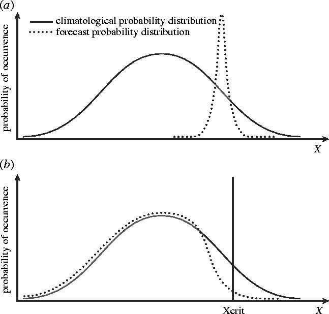
(a) The solid line is a schematic illustration of the climatological probability of some climatic variable, such as seasonal-mean surface temperature for some part of the tropics. The dashed line is a schematic illustration of a seasonal forecast probability distribution showing clear predictability. (b) as (a) but for a forecast probability distribution whose overall level of predictability is small. However, for certain applications which require knowledge of whether or not temperature exceeds some threshold, there may be significant predictability.

Now suppose we have a forecast system that predicts the probability distribution of summer-mean temperature for this part of the tropics, a season ahead. Such a system is necessarily based on the ensemble forecast methodology, discussed below. Suppose that such a system predicts, for a particular summer, the dashed curve in figure 2a. The two probability distributions are clearly different, indicating unambiguous predictability for this summer's prediction: that the seasonal-mean temperature will be above average.

What about the situation in figure 2b? Throughout most of the temperature range, the difference between the forecast probability distribution and the climatological probability distribution is small. As such, we might be inclined to say that in this situation, predictability is rather small. But suppose we are mainly interested in the prevalence of a certain weather-sensitive disease, call it ‘X’, which only becomes prevalent if the temperature exceeds some threshold T_c, or suppose that some crop ‘Y’ fails if temperature exceeds T_c. Then for these health and agricultural applications, this particular forecast probability distribution would imply very useful and important predictability: that the probability of disease X becoming prevalent or of crop Y failing, is predicted to be very small in the coming season.

These two specific examples (X and Y) are simplistic; however, the point is that assessment of whether predictability exists or not is inherently linked to the applications for which the seasonal forecasts are being used. Indeed, this motivates a plausible definition of predictability: a variable x is predictable if the forecast probability distribution of x differs sufficiently from the climatological probability distribution to influence relevant decision makers.

4. Ensemble weather prediction

As discussed above, atmospheric evolution is chaotic, i.e. sensitive to initial-condition uncertainty. However, with modern-day supercomputers, we can run weather forecast models many times from very slightly different initial conditions, consistent with the uncertainties—at the European Centre for Medium-range Weather Forecasts (ECMWF), the Wedium-range Forecast model is run 52 times twice a day—to estimate the effect of this initial-condition uncertainty. The resulting forecasts can be combined to produce a forecast probability distribution.

Figure 3 is an example of a 42 h ensemble forecast for the infamous and highly damaging storm Lothar of December 1999. ECMWFs main high-resolution deterministic forecast completely missed this storm. In this particular case, the spread of the ECMWF ensemble was enormous, indicating that the development of the flow was highly unpredictable. However, despite this unpredictability, the ensemble did indicate a significant probability, or risk, of a severe weather event. Of course, 42 h weather forecasts are not normally this unpredictable.

Figure 3.

Surface pressure ‘stamp maps’ for the 42 h ECMWF ensemble forecast for the severe storm Lothar.

The scientific basis for ensemble forecasting can be demonstrated using equation (2.1). The evolution of three different ensembles is shown in figure 4. Because the underlying equations are nonlinear, the growth of initial uncertainty is strongly dependent on the starting conditions. The practical point of this is that the predictability of forecasts is variable; we need ensembles to tell us in advance how predictable the climate system is.

Figure 4.

The scientific basis for ensemble forecasting illustrated using the prototypical Lorenz (1963) model of low-order chaos, showing that in a nonlinear system predictability is flow-dependent.

5. Climate prediction on seasonal time-scales

Let us now return to the problem of climate prediction. As discussed (see http://www.clivar.org), the physical basis for seasonal climate prediction lies in components of climate that vary slowly compared with individual weather events—that is to say ocean and land surface (including, cryospheric components). As is well known, El Niño is the prototypical phenomenon with predictability on the seasonal time-scale. Fully coupled ocean–land–atmosphere models are required in order to predict seasonal climate by dynamical means. Just as in weather prediction, ensemble forecasts using these coupled models give probabilistic risk forecasts of climate events. However, for seasonal ensemble prediction it is essential to take into account not only uncertainty in the initial conditions, but also uncertainty in the model equations themselves. Uncertainty in model equations arises because the process of parameterization, the way in which sub-gridscale motions are represented in weather and climate models, is not a precisely defined procedure (Palmer et al. 2005).

One way to represent model uncertainty is to incorporate, within the ensemble, independently derived models. The resulting ensemble prediction system is known as a multi-model ensemble system (see below). There are other ways to represent model uncertainty, e.g. stochastic physics (see Buizza et al. 1999; Palmer 2001) and the perturbed-parameter approach (see Murphy et al. 2004; Stainforth et al. 2005).

The skill and utility of multi-model ensemble forecast systems has been explored in a recent European Union project called DEMETER; Palmer et al. 2004. (Demeter was the Greek Goddess of Fertility. When her daughter Persephone was abducted into the underworld, Demeter cast a deep freeze on the earth, so that no crops would grow. Eventually, Zeus intervened and Persephone was allowed out for 9 months of the year. Demeter kept the freeze on the Earth for the remaining 3 months. Without Demeter we would not have seasons, and hence seasonal forecast projects! More prosaically, DEMETER stands for ‘Development of a European Multi-Model Ensemble System for Seasonal to Inter-annual Climate Prediction’.) In this project, advantage was taken of one of the real strengths of European climate research: the existence of seven quasi-independent state-of-the-art comprehensive global climate models developed at a number of institutes around Europe.

Figure 5 gives an example of how the DEMETER multi-model forecast system produces more reliable seasonal forecasts than is possible using a single-model ensemble system. Shown are 2–4 month forecasts of El Niño sea surface temperature anomalies over the period 1980–2001. The solid dot shows the observed El Niño sea surface temperature anomaly, the ‘bar and whiskers’ show the forecast probability distribution of El Niño sea surface temperature anomaly in terms of terciles. Forecasts at the top of figure 5 are based on the ECMWF model only. While there is clear skill, this single-model ensemble system is not fully reliable, there are many cases where the verification lies outside the range of the ensemble. The bottom diagram is for the full DEMETER multi-model ensemble system; now the verification almost always lies with the range of the ensemble. This is one example of many that show conclusively that the DEMETER ensemble is intrinsically more useful and more skilful than forecasts from any one (e.g. national) model (Hagedorn et al. 2004; Doblas-Reyes et al. 2005).

Figure 5.

(a) Seasonal forecast probability distributions of El Niño based on the ECMWF model within the DEMETER project; bar and whiskers give tercile distributions and grey diamonds give ensemble mean. The solid dot gives the observed value, which often lies outside the forecast. (b) As top but for the DEMETER multi-model ensemble. The validation now almost always lies within the ensemble. The probabilistic skill of the DEMETER multi-model ensemble is greater than for the single-model ensemble.

A key part of the DEMETER project was to demonstrate value for applications in health and agriculture. In order to study this quantitatively, a system was developed using partners expert in downscaling, and partners expert in malaria prediction, on the one hand, and crop modelling on the other. Figure 6 is an example of the month 2–4 DEMETER forecast probability distribution of malaria prevalence for a grid point in southern Africa (Morse et al. 2005). As with the El Niño sea surface temperature distribution, terciles of the forecast probability distribution are shown. There is some clear year-to-year variability, and the ‘verification’ (here based on running the malaria model using ERA-40 weather) lies within the forecast ensemble.

Figure 6.

Forecast probability distributions (bar and whiskers showing terciles) of malaria prevalence over southern Africa, based on the DEMETER multi-model ensemble system coupled to a malaria prediction model. The diamond denotes the ensemble-mean value, and the solid dot denotes malaria prevalence when the malaria model is forced with ERA-40 gridded analyses (so-called tier-2 validation; Morse et al. 2005).

Recently, the use of the DEMETER system for malaria prediction for Botswana has been studied (Thomson et al. in press). It is concluded that it is now possible to realize the aspiration of the Abuja Declaration of African Health ministers, to provide a malaria early warning system ahead of the start of the rainy seasons.

Figure 7 shows month 2–4 forecast probability distributions from DEMETER, but here based on wheat yield in tons per hectors over specific European countries (Canteloube & Terres 2005; see also Marletto et al. 2005). While only a limited number of years have so far been studied, there is evidence of useful predictability and the DEMETER forecasts have proven more skilful than forecasts made using statistical empirical techniques by the European Commission's own crop forecasters.

Figure 7.

Probability distributions of wheat yield for different countries (a) France, (b) Germany, (c) Denmark and (d) Greece in Europe, based on DEMETER multi-model re-forecasts (from Canteloube & Terres 2005). The open dot denotes the ensemble mean value, and the solid dot denotes crop yield when the crop model is forced with ERA-40 gridded analyses. The bars denote the Eurostat yield.

DEMETER data is also of value for crop yield prediction in the tropics (groundnut yields in Western India; Challinor et al. 2005). Also, in collaboration with the Georgia Institute of Technology and the Bangladesh Meteorological Institute, the skill of the DEMETER forecasts coupled to hydrological models for the Bangladesh drainage basins, are being used to forecast probability distributions of flooding in Bangladesh (Webster et al. 2005).

Scientists who wish to assess the extent to which there is useful predictability for their part of the world for particular applications of interest are strongly encouraged to go to the DEMETER web site (http://www.ecmwf.int/research/demeter). All of the DEMETER data can be freely downloaded from this web site, as can the ERA-40 data used for validations.

6. Forecasting climate change

Multi-model ensemble forecasts have also been used to make probabilistic climate change forecasts (Palmer & Räisänen 2002). Such ensemble forecasts will play a role in the forthcoming fourth assessment report of the Intergovernmental Panel on Climate Change (IPCC: http://www.ipcc.ch).

A multi-model multi-scenario ensemble (based on 15 models and three scenarios) has been recently created for the IPCC fourth assessment report (http://ipcc-wg1.ucar.edu/meetings/CMSAW). Using this ensemble, we show in figure 8 an analysis of the probability of occurrence of an extremely warm June–August (JJA) temperature over Africa and Europe during the period 2081–2100. Here ‘extremely warm’ is defined as a season-mean temperature whose probability of occurrence according to the twentieth century control integrations of the multi-model ensemble is 5% or less.

Figure 8.

Probability of extremely warm JJA temperatures in 2081–2100 based on a multi-model multi-scenario ensemble, assuming each member of the ensemble to be equally likely. An extremely warm JJA is one whose temperature lies in the 95th percentile category according to twentieth century control simulations. Details to be found in Weisheimer & Palmer (to appear).

Figure 8 shows a fairly heterogeneous picture in the probability of extremely warm temperature between 2081 and 2100. Over parts of the west coast of southern Africa, the probability of an extremely warm boreal summer is predicted to increase from 5 to about 10%; that is such summers which occurred about once every 20 years in the twentieth century, can be expected to occur about once every 10 years. On the other hand, there are regions (e.g. bordering the Gulf of Guinea and the Mediterranean) where extremely warm boreal summers are expected to occur with a probability of more than 60%. In these regions, such (twentieth century) extremes can be expected in at least two seasons out of three. In general, the increase in the probability of an extreme JJA arises both because of a shift towards higher temperatures and a broadening of the multi-model-based probability distribution. The reliability of these results have been examined using the bounding box diagnostic developed by Weisheimer et al. (2005) to study the DEMETER seasonal climate forecasts. Interestingly, those land areas with the highest expected change in the occurrence of extreme warm seasons are also most reliable. For further details, see Weisheimer & Palmer (in press).

Analysis of extremely wet and extremely dry season is in progress using similar techniques and based on this multi-model ensemble. Results will be reported in due course.

7. Conclusions

In this paper, we have discussed the reasons for predicting climate, and the use of multi-model ensembles for making seasonal climate predictions and predictions of climate change.

In this paper, we have not tried to apply non-uniform weighting to the members of the ensemble (e.g. Doblas-Reyes et al. 2005). In principle, non-uniform weighing is appropriate when the members of the ensemble have unequal skill or simulation capability. Similarly, we have not discussed alternate methods for representing model uncertainty, e.g. using perturbed parameter ensembles (Murphy et al. 2004; Stainforth et al. 2005) or stochastic physics ensembles (Buizza et al. 1999; Palmer 2001). Different techniques for representing model uncertainty are compared in Palmer et al. (2005). It is one of the objectives of the EU FP6 project ENSEMBLES to inter-compare these methods through seasonal and decadal-time-scale integrations.

Whatever the method used to represent model uncertainty, the key point is that the climate forecast community is now capable of producing ensemble forecasts the output from which can be fed to application models, in health, agriculture and hydrology, thus producing useful forecast probability distributions for application variables.

References

- Buizza R, Miller M.J, Palmer T.N. Stochastic simulation of model uncertainties in the ECMWF ensemble prediction system. Q. J. R. Meteorol. Soc. 1999;125:2887–2908. doi:10.1256/smsqj.56005 [Google Scholar]
- Canteloube P, Terres J.-M. Seasonal weather forecasts for crop yield modelling in Europe. Tellus A. 2005;57:476–487. doi:10.1111/j.1600-0870.2005.00125.x [Google Scholar]
- Challinor A.J, Slingo J.M, Wheeler T.R, Doblas-Reyes F.J. Probabilistic simulations of crop yield over western India using the DEMETER seasonal hindcast ensembles. Tellus. 2005;57A:498–512. [Google Scholar]
- Doblas-Reyes F.J, Hagedorn R, Palmer T.N. The rationale behind the success of multi-model ensembles in seasonal forecasting—II calibration and combination. Tellus A. 2005;57:234–252. doi:10.1111/j.1600-0870.2005.00104.x [Google Scholar]
- Hagedorn R, Doblas-Reyes F.J, Palmer T.N. The rationale behind the success of multi-model ensembles in seasonal forecasting—I. Basic concept. Tellus A. 2004;57:219–233. doi:10.1111/j.1600-0870.2005.00103.x [Google Scholar]
- Lorenz E.N. Deterministic non-periodic flow. J. Atmos. Sci. 1963;42:433–471. [Google Scholar]
- Marletto, Zinoni F, Criscuolo L, Fontana G, Marchesi S, Morgillo A, Van Soetendael M.R.M, Ceotto E, Anderson U. Evaluation of downscaled DEMETER multi-model ensemble seasonal hindcasts in Northern Italy by means of a model of wheat growth and soil water balance. Tellus A. 2005;57:488–497. doi:10.1111/j.1600-0870.2005.00109.x [Google Scholar]
- Morse A.P, Doblas-Reyes F.J, Hoshen M.B, Hagedorn R, Thomson M.C, Palmer T.N. First steps towards the integration of a dynamic malaria model within a probabilistic multi-model forecast system. Tellus A. 2005;57:464–475. doi:10.1111/j.1600-0870.2005.00124.x [Google Scholar]
- Murphy J.M, et al. Quantifying uncertainties in climate change using a large ensemble of global climate model predictions. Nature. 2004;430:768–772. doi: 10.1038/nature02771. doi:10.1038/nature02771 [DOI] [PubMed] [Google Scholar]
- Palmer T.N. A nonlinear dynamical perspective on model error: a proposal for nonlocal stochastic–dynamic parametrisation in weather and climate prediction models. Q. J. R. Meteorol. Soc. 2001;127:685–708. doi:10.1256/smsqj.57201 [Google Scholar]
- Palmer T.N, Räisänen J. Quantifying the risk of extreme seasonal precipitation events in a changing climate. Nature. 2002;415:512. doi: 10.1038/415512a. doi:10.1038/415512a [DOI] [PubMed] [Google Scholar]
- Palmer T.N, et al. Development of a European multi-model ensemble system for seasonal to inter-annual prediction. Bull. Am. Meteorol. Soc. 2004;85:853–872. doi:10.1175/BAMS-85-6-853 [Google Scholar]
- Palmer T.N, Shutts G.J, Hagedorn R, Doblas-Reyes F.J, Jung T, Leutbecher M. Representing model uncertainty in weather and climate prediction. Annu. Rev. Earth Planet Sci. 2005;33:163–193. doi:10.1146/annurev.earth.33.092203.122552 [Google Scholar]
- Stainforth D.A, et al. Uncertainty in predictions of the climate response to rising levels of greenhouse gases. Nature. 2005;433:403–406. doi: 10.1038/nature03301. doi:10.1038/nature03301 [DOI] [PubMed] [Google Scholar]
- Thomson, M. C., Doblas-Reyes, F. J., Mason, S. J., Hagedorn, R., Connor, S. J., Phindela, T., Morse, A. P. & Palmer, T. N. In press. Malaria early warnings based on seasonal climate forecasts from multi-model ensembles. Nature [DOI] [PubMed]
- Webster P.J, Anderson D.L.T, Chang H.-R, Grossman R, Hoyas C, Hopson T, Shami K, Subbiah A, Palmer T.N. Regional application of monsoon dynamics: implementation of a three-tier flood and precipitation forecasting scheme for Bangladesh and surrounding regions. CLIVAR Exchanges. 2004;9:21–25. [Google Scholar]
- Weisheimer, A. & Palmer, T. N. In press. Changing frequency of occurrence of extreme seasonal temperatures due to global warming. Geophys. Res. Lett.
- Weisheimer A, Smith L.A, Judd K. A new view of seasonal forecast skill: bounding boxes from the DEMETER ensemble forecasts. Tellus A. 2005;57:265–279. doi:10.1111/j.1600-0870.2005.00106.x [Google Scholar]